A New Visualization and Analysis Method for a Convolved Representation of Mass Computational Experiments with Biological Models

Abstract

Modern computational biology makes widespread use of mathematical models of biological systems, in particular systems of ordinary differential equations, as well as models of dynamic systems described in other formalisms, such as agent-based models. Parameters are numerical values of quantities reflecting certain properties of a modeled system and affecting model solutions. At the same time, depending on parameter values, different dynamic regimes—stationary or oscillatory, established as a result of transient modes of various types—can be observed in the modeled system. Predicting changes in the solution dynamics type depending on changes in model parameters is an important scientific task. Nevertheless, this problem does not have an analytical solution for all formalisms in a general case. The routinely used method of performing a series of computational experiments, i.e., solving a series of direct problems with various sets of parameters followed by expert analysis of solution plots is labor-intensive with a large number of parameters and a decreasing step of the parametric grid. In this regard, the development of methods allowing the obtainment and analysis of information on a set of computational experiments in an aggregate form is relevant. This work is devoted to developing a method for the visualization and classification of various dynamic regimes of a model using a composition of the dynamic time warping (DTW-algorithm) and principal coordinates analysis (PCoA) methods. This method enables qualitative visualization of the results of the set of solutions of a mathematical model and the performance of the correspondence between the values of the model parameters and the type of dynamic regimes of its solutions. This method has been tested on the Lotka–Volterra model and artificial sets of various dynamics.

1. Introduction

Modern computational biology is using mathematical models of biological systems, in particular systems of ordinary differential equations (ODE) [1,2,3] and partial differential equations (PDE) [3,4], as well as models of dynamic systems described in other formalisms, such as agent-based models [5,6,7,8,9,10], Boolean networks [11,12] and cellular automata [13,14]. Parameters are numerical values of quantities reflecting certain properties of a modeled system and affecting model solutions. At the same time, depending on the parameter values, different dynamic modes—nonstationary, oscillatory, chaotic, and stationary, established as a result of transient modes of various types—can be realized in the system.

Parametric sensitivity analysis is one of the important tasks in the study of mathematical models of biological objects and processes [15]. Nevertheless, not for all formalisms does the prediction of changes in the type of solution dynamics depending on changes in model parameters have an analytical solution. Often, practiced visual analysis of multiple plots of solutions, corresponding to different sets of parameters, is difficult with a large number of parameters and a fine-grained parametric grid. In this connection, it is relevant to develop methods that allow obtaining and analyzing information about the set of computational experiments in an aggregate form, reflecting the essential characteristics of solutions, such as the type of dynamic mode, as well as carrying out a visual analysis of the parametric space of the model under study [16].

Modern computational biology relies heavily on mathematical methods for building and analyzing models of biological systems and information technologies that allow mass computational experiments using supercomputers. Specialized information systems and databases such as Biomodels [17], JWS Online [18], CellML Model Repository [19], BiGG Models [20], EcoBase [21], etc., contain hundreds and thousands of models of biological systems from metabolic reactions and gene networks to population and ecosystem models. At the same time, the parametric study of models of biological systems is one of the most labor-intensive and weakly automated problems, the analytical possibilities of solving which are very limited due to the essential nonlinearity of the dynamical systems under study. Since models of molecular–genetic systems described in terms of ordinary differential equations often contain dozens of equations and hundreds of parameters, the empirical investigation of the parametric stability of the solutions of these ODE systems leads to the consideration of thousands of calculation scenarios, which requires considerable computing power using supercomputers and limits the resolution of the parametric grid in question. In addition, calculations using more detailed parametric grids produce large amounts of model data, the direct understanding of which is difficult and requires the use of big data analysis methods. Similar problems are encountered when considering problems related to solution stability and structural stability of models.

There is a certain range of analytical approaches to this problem that can be applied to a number of special cases, such as models described in terms of ordinary differential equations or when solving a certain class of problems [22,23,24]. Among these approaches are local and global parametric sensitivity analysis, stability analysis by equipotential curves, classical methods of stability analysis by first approximation and system roughness analysis [25,26].

At the same time, the direct calculation of a series of direct problems can act as a method for conducting a computational experiment capable of providing useful information about the nature of the dynamic system and its solutions in cases where the use of analytical methods turns out to be difficult for some reason. However, understanding the information obtained in the course of such computational experiments requires “convolution” of calculation results and their presentation in a compressed form that allows extracting knowledge from large volumes of simulation data. Therefore, the development of methods for the analysis of mass computational experiments for models of biological systems is of particular importance for applied research.

This work is devoted to developing a new method of visualization and analysis of the results of mass computational experiments using models of biological systems, which demonstrate different dynamic regimes. The main idea underlying the proposed method is to obtain compressed representation of the results of such computational experiments via the composition of an algorithm for dynamic time warping (DTW algorithm) and principal coordinates analysis (PCoA). Such a method allows the qualitative visualization of the results of the set of solutions of a mathematical model and the performance of a correspondence between the values of the model parameters and the type of dynamic regimes of its solutions.

2. Materials and Methods

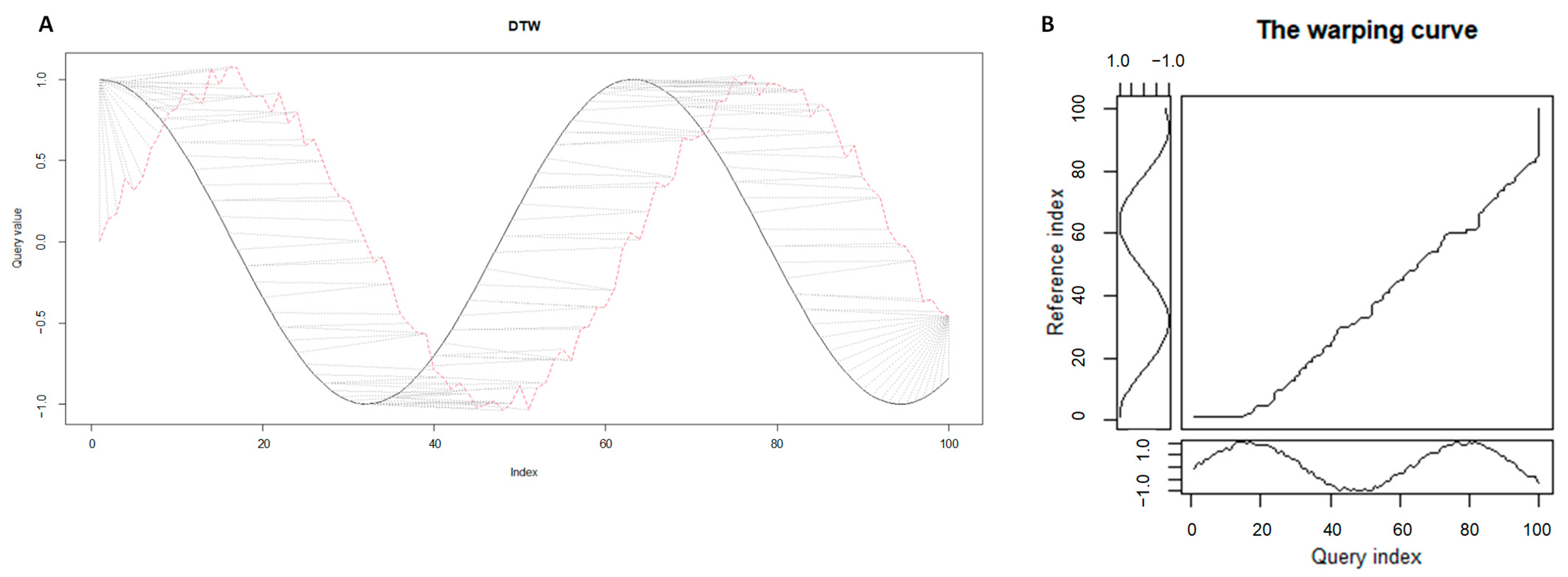
2.1. Time series Analysis with Dynamic Time Warping Algorithm

2.1.1. Formulation of Time Series Alignment Problem

Dynamic time warping [27] is a method for comparing time series, which provides both a distance measurement insensitive to local compression and stretching and an optimal deformation of one of the two input series on the other. The algorithms of calculation of time series alignments are implemented in different statistical packages, in particular, in the package dtw of R [28]. This package allows the computation of time series alignment by freely mixing various continuity constraints, endpoints, distance definitions, and other functionalities.

The purpose of DTW, as a class of algorithms for comparing time series against each other, is, given two time series, to stretch (compress) them locally, making one as similar as possible to the other. The distance between them is calculated after stretching by summing the distances between the individual aligned elements (see Figure 1).

The types of DTW algorithms differ in the space of input features, the assumed local distance, the presence of local and global alignment constraints, and some other parameters. This freedom makes DTW a very flexible approach to alignment.

The task of alignment of two time series can be formulated as follows. It is required to compare two time series: $X=\left(x_1,...,x_N\right),Y=(y_1,...,y_M).$ For the sake of clarity in the future, we will keep $i=1...N$ to index the elements in the $X$ and $j=1...M$ in $Y$ respectively. We also assume that the non-negative local distance function $f$ is defined for any pair of elements $x_i$ and $y_j$:

$$d\left(i,j\right)=f(x_i,y_j)\ge 0,$$

(1)

where $d\left(i,j\right)$ represents the corresponding elements of the distance matrix between the vectors $X$ and $Y.$ Therefore, further discussion, without limiting generality, applies to cases where $X$ and $Y$ are unidimensional or multidimensional, as long as $f(·,·)$ is defined accordingly. The most common choice is to take the Euclidean distance, while other distance definitions may also be useful. The technique is based on the warping curve $\phi \left(k\right),k=1...T$:

$$\phi \left(k\right)=\left({\phi }_x\right(k),{\phi }_y(k\left)\right),where$$

$${\phi }_x\left(k\right)\in \left\{1...N\right\},$$

$${\phi }_y\left(k\right)\in \left\{1...M\right\}$$

$$T=\mathrm{m}\mathrm{a}\mathrm{x}\{N,M\}$$

For the warping functions ${\phi }_x$ and ${\phi }_y$ the time indexes are reassigned $X$ and $Y$ respectively. Taking into account $\phi$, we calculate the average accumulated distortion between the warped time series $X$ and $Y$:

$$d_{\phi }\left(X,Y\right)={\sum }_{k=1}^T\frac{d\left({\phi }_x\left(k\right),{\phi }_y\left(k\right)\right)m_{\phi }\left(k\right)}{M_{\phi }}$$

(2)

where $m_{\phi }\left(k\right)$ is the weighting factor for each step, and $M_{\phi }$ is the respective normalizing constant to ensure the comparability of the accumulated distortions at different paths (see Section 2.1.2). The value $M_{\phi }·d_{\phi }(X,Y)$ stores the total (non-normalized) alignment cost. At $\phi$ constraints are usually imposed, such as monotonicity, to preserve the temporal order and avoid meaningless cycles:

$${\phi }_x\left(k+1\right)\ge {\phi }_x\left(k\right)$$

$${\phi }_y\left(k+1\right)\ge {\phi }_y\left(k\right)$$

Thus, the idea underlying the DTW algorithm can be stated more formally as follows: find such an optimal alignment $\phi$, such that

$$D\left(X,Y\right)=\underset{\phi }{\min }{d}_{\phi }(X,Y),$$

(3)

where $d_{\phi }$—average accumulated distortion value between time series $X$ and $Y$, calculated according to the Formula (2). $D\left(X,Y\right)$ is the DTW distance.

In other words, the renumbering of vector elements is chosen for $X$ and $Y$, which makes them as close to each other as possible. The spatial and temporal complexity of the DTW algorithm is quadratic: $O(N·M).$ At the output of the DTW algorithm, one can obtain different data on the analyzed time series, in particular the value of the function $D\left(X,Y\right)$—minimum global “dissimilarity”, or “DTW distance”. The shape of the warping curve $\phi$ will provide information about the pairwise correspondences of the time moments (see Figure 1B). In places where the warping curve has a diagonal shape, there is an element-by-element correspondence. Thus, the warping function can be used to estimate the consistency of the two time series and measure the corresponding distortions.

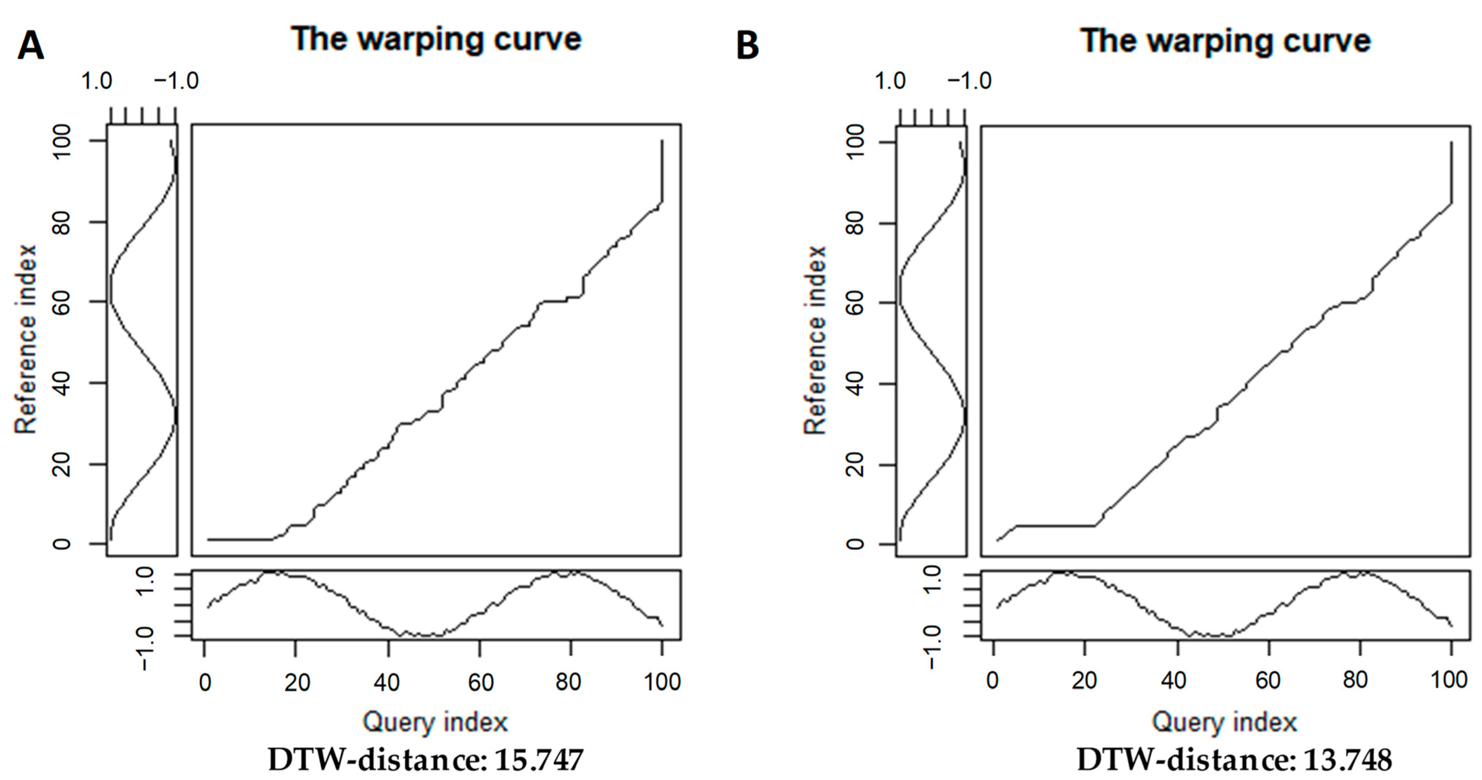
2.1.2. Time Series Alignments: Samples of Step Patterns and Local Slope Constraints for the Warping Curves

To calculate the alignment, we used the function dtw() with the parameters of the global alignment without windows (global constraints) and Euclidean distance. The calculation of global alignments means that the heads and tails of the time series should match each other. In other words, the following constraints are imposed on the endpoints:

$${\phi }_x\left(1\right)={\phi }_y\left(1\right)=1;$$

(4)

$${\phi }_x\left(T\right)=N; {\phi }_y\left(T\right)=M.$$

(5)

Conditions (4) and (5) can be relaxed, which is of practical importance, in particular, for aligning the dynamics of solutions obtained using different initial data.

Usually, when using the DTW algorithm, it is required to limit the number of consecutive elements that are “skipped” in any time series, i.e., remain unmatched. It is worth noting that skipping elements is often completely prohibited by the continuity constraint, which implies that all elements must be matched:

$$\left|{\phi }_x\left(k+1\right)-{\phi }_x\left(k\right)\right|\le 1,$$

(6)

$$\left|{\phi }_y\left(k+1\right)-{\phi }_y\left(k\right)\right|\le 1$$

(7)

Alignments are usually achieved by duplicating elements, i.e., by allowing a single time point in X to match several consecutive elements in Y, or vice versa. How many repeating elements can be matched consecutively or how many can be skipped is set by constraints on the local slope of the warping curve. This property can be controlled by a flexible scheme called step patterns. Step patterns determine the sets of allowed transitions between matched pairs and corresponding weights. In other words, step patterns define allowable values for $\phi (k+1)$ given $\phi \left(k\right),\phi \left(k-1\right),$ etc. It is useful to note that DTW has no additional penalties for duplicate or skipped elements, as other alignment algorithms (e.g., Smith–Waterman [29], Levenshtein [30] or Needleman–Wunsch [31]).

From a step pattern, one can define an explicit form of a recursive relationship that selects the location for the next point of the warping curve with the current and previous points already obtained. The step patterns commonly used in DTW analysis include symmetric1, symmetric2, asymmetric and Rabiner-Juang step patterns. The explicit form of the corresponding recursive relations is presented in the

Table 1. The recursion formulae for the step patterns used in this work. $d\left(i,j\right)$—local distance, $g(i,j)$—the average accumulated distortion value obtained at the k-th step, $i,j$—the indices of the cell where to go in the matrix of local distances under the constraints of the corresponding pattern.

Step Pattern	Recursion Formula
symmetric1	$g\left(i,j\right)=\min \{g\left(i-1,j-1\right)+d\left(i,j\right),$ $g\left(i,j-1\right)+d\left(i,j\right),$ $g\left(i-1,j\right)+d\left(i,j\right)\}$
symmetric2	$g\left(i,j\right)=\min \{g\left(i-1,j-1\right)+2\cdot d\left(i,j\right),$ $g\left(i,j-1\right)+d\left(i,j\right),$ $g\left(i-1,j\right)+d\left(i,j\right)\}$
asymmetric	$g\left(i,j\right)=\min \{g\left(i-1,j\right)+d\left(i,j\right),$ $g\left(i-1,j-1\right)+d\left(i,j\right),$ $g\left(i-1,j-2\right)+d\left(i,j\right)\}$
Rabiner-Juang	$g\left(i,j\right)=\min \{g\left(i-2,j-1\right)+d\left(i-1,j\right)+d\left(i,j\right),$ $g\left(i-2,j-2\right)+d\left(i-1,j\right)+d\left(i,j\right),$ $g\left(i-1,j-1\right)+d\left(i,j\right),$ $g\left(i-1,j-2\right)+d\left(i,j\right)\}$

.

For the graphical schemes representing the step patterns mentioned in Table 1 one can refer to [28]. Thus, the step patterns determine the feasible moving directions on the matrix of local distances and the weight of each move (step cost $m_{\phi }$), which altogether allows the calculation of the optimal average accumulated distortion between the two time series, i.e., the DTW distance between the aligned curves.

For standard symmetric2 recursion, the average step cost is calculated by dividing the total distance by the normalization constant $N+M$, where N is the length of the query sequence and M is the length of the reference sequence. Other step patterns require their own normalization formulas (constants), which is $M_{\phi }$ in Formula (2). Classical step patterns are classified according to their symmetry (symmetric/asymmetric) and the constraints imposed on the slope. Consider how the warping curve and DTW distance change when the step pattern is changed from symmetric2 to asymmetric to align the two time series (see Figure 2).

Using a different step pattern to calculate the DTW distance, one can obtain a slightly different distance value and a smoother warping curve, which allows the conclusion that the given time series are closer to each other. The choice of different step patterns allows the adjustment of the DTW algorithm to more accurately reflect the nature of similarity or difference of the analyzed time series.

2.2. Dimensionality Reduction during Metric Multidimensional Scaling Using Principal Coordinate Analysis

The analysis of experimental data describing the object of study as a set of measured features is a topical task in molecular biology, ecology and biomedicine, as well as in a number of other disciplines [32,33]. In such situations, it is advisable to use general methods designed to visualize the data structure, in particular methods of dimensionality reduction, or ordination, methods, such as methods of factor analysis, multivariate scaling and, in particular, the method of principal coordinates [34]. The most effective use of ordination methods is when it is possible to represent the original information using one, two, or three dimensions. In this case, it is possible to represent the data set graphically, which allows the visualization of the nature of the sample under study.

In practical tasks, the aim of applying dimensionality reduction methods can be both the visualization of the relative positioning of objects and more specific applications. Among them includes dividing the initial information into homogeneous groups (clusters) or revealing the inner dimensionality of a variety, in whose neighborhood the main data mass is concentrated. Moreover, if the partitioning into groups is already known, the relevant task is to find such a mapping into a space of smaller dimensionality, at which the partitioning into groups is best preserved [35]. One of the most widely used ordination methods for the visualization of multivariate data is the principal component analysis (PCA [36]). This method uses object-feature matrices or correlation matrices of the original variables. However, more than half a century ago, Gower proposed [37] an ordination method, based not on the correlation matrix of raw data but on the matrix of pairwise distances between objects, which he called principal coordinate analysis (PCoA). This method is very useful in practice when the number of objects is much smaller than the number of features, which is becoming increasingly routine in biological research, especially in molecular biology.

Principal coordinate analysis (PCoA), or metric multidimensional scaling (MDS), is a dimensionality reduction method similar to PCA. Its advantage over PCA is that it can use any similarity difference measure (such as Jaccard’s index, Bray–Curtis dissimilarity, and other commonly used ecological measures), not just the Euclidean distance. PCoA is well suited for visualizing patterns in the samples under study without making a priori hypotheses about the structure of the data, and allows more flexibility in circumventing the problem of missing values by selecting an appropriate measure of difference [35,38]. In addition, PCoA can handle matrices that include both quantitative, rank and qualitative variables. Thus, PCoA is a dimensionality reduction method that allows using an arbitrary similarity/difference measure to analyze and visualize multivariate samples.

The scheme of the principal coordinates analysis is as follows. Suppose there are data objects located in multidimensional space described by a distance or dissimilarity matrix between those objects. It is necessary to project them on a space of lower dimensionality, for example, one- or two-dimensional space, in such a way as to maximally preserve the information on the distance between the original points. The axes of the two-dimensional space, on which the points are projected, are called principal coordinates. Thus, the procedure calculates the geometric coordinates of the objects in a new space of lower dimension. Formally, we minimize the stress function, which consists of the sum of the absolute values of the distances between points in n-dimensional space and the same points projected onto 1-, 2-, or more-dimensional principal coordinate space:

$$\sum _{i=1}^n\left|d_i-\widehat{d_i}\right|\to \min ,$$

(8)

where $d_i$ represents the point−to−point distances $x_{i_l} \mathrm{a}\mathrm{n}\mathrm{d} x_{i_k}$ in n-dimensional space, and $\widehat{d_i}$ represents the distances between the same points in the principal coordinate space. PCoA allows one to obtain a set of uncorrelated axes sorted by the amount of explained variance between the source data points in a similar way that PCA does (more details on the mathematical rationale behind the PCoA method can be found in [39]).

Thus, principal coordinate analysis allows us to visually assess the mutual location of the analyzed objects on the basis of a certain measure of dissimilarity or distance applied to the data. In this paper, we apply this method, taking the DTW distance as the metric. The idea of using methods of dimensionality reduction, in particular, principal component analysis, to display a set of similar function plots has been discussed in the literature before [40]; however, combining it with the DTW algorithm to map many different solutions, to the best of our knowledge, is described here for the first time.

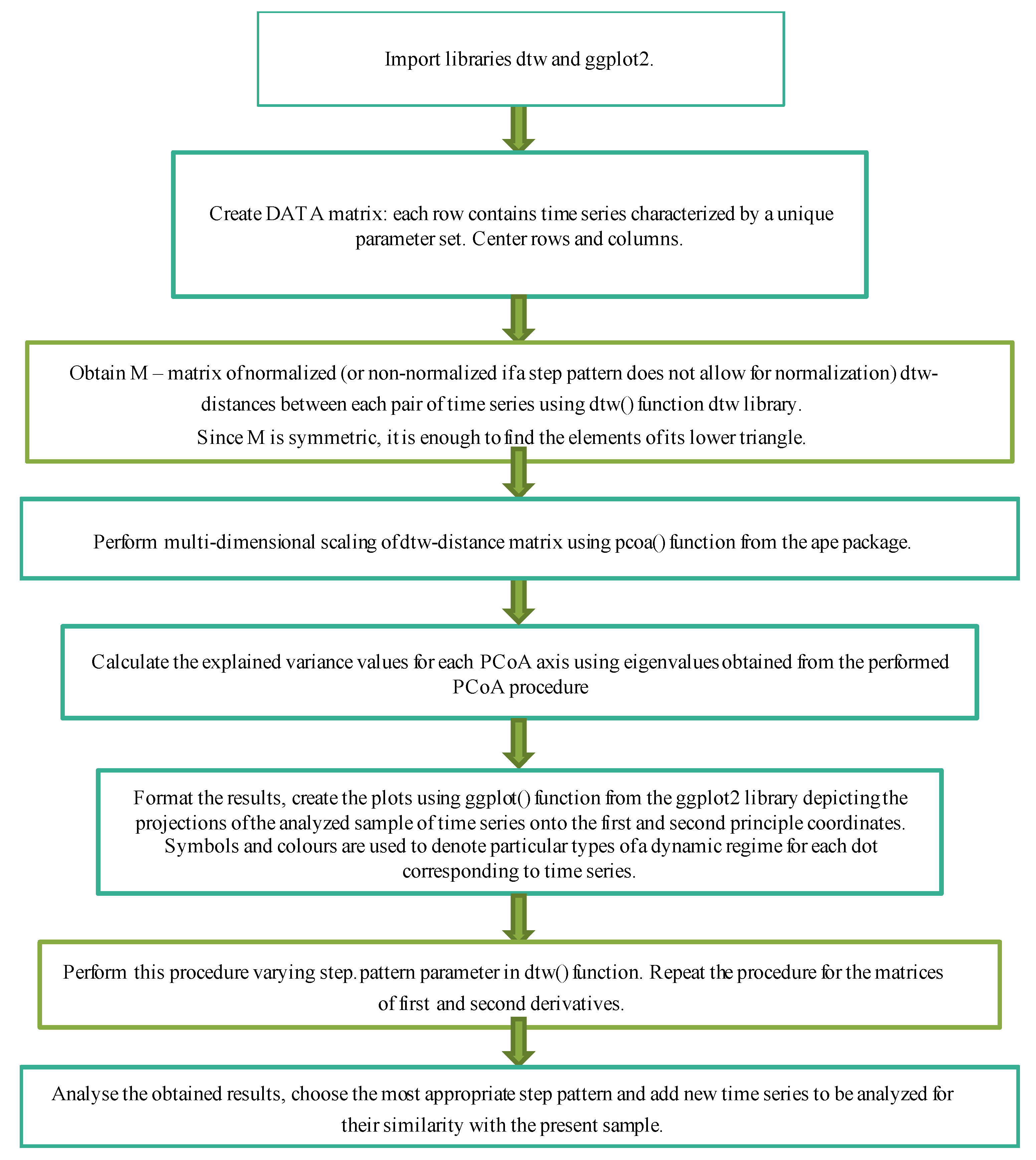
2.3. DTW+PCoA-Based Method for a Convolved Representation of Mass Computational Experiments

The stages of analysis performed in R are represented in the form of a scheme of the corresponding analytical pipeline (see Figure 3).

Thus, the approach to the analysis of visualization and classification of various dynamic modes of arbitrary models of dynamic systems, described in the work, consists in the following (the graphical scheme of the software pipeline used in this work can be found in Figure S1 in Supplementary Materials):

• to perform computational experiments with different sets of parameters under consideration;
• to obtain a matrix of DTW distances between all samples;
• to apply principal coordinates analysis to it;
• to qualitatively analyze the obtained results for each of the parameters or for the whole set, determining how the types of dynamic regimes of the model change depending on changes in its parameters.

Model curves for method calibration were generated in the package of the applied mathematical program Scilab. The Lotka–Volterra model has been realized by means of Scilab on time interval [0;1000], initial conditions–point (5;2). The used method of numerical integration is Runge–Kutta of the 4th order of accuracy.

3. Results

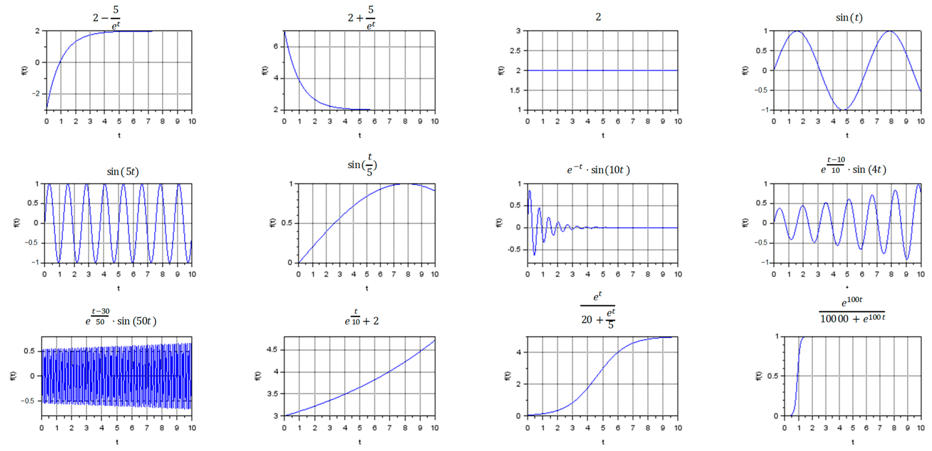
3.1. Visualization of Different Types of Dynamic Regimes

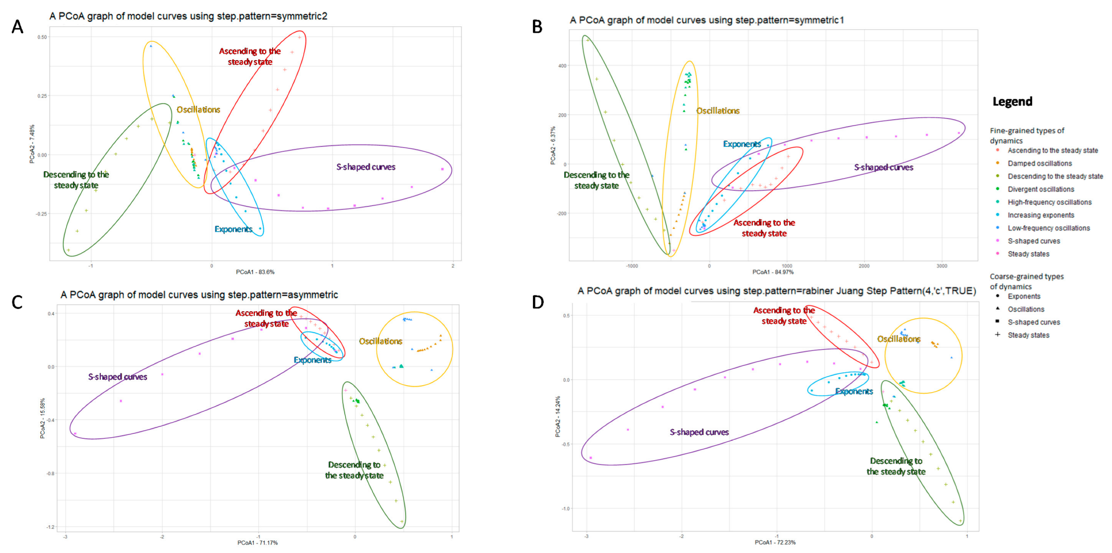
3.1.1. A Basic Application of DTW+PCoA-Based Method with Various Step Patterns

To calibrate the proposed method, we considered the problem of visualizing a set of artificially generated model curves implementing different types of dynamic regimes (see Figure 4).

Within the framework of this study, we distinguish the following types of dynamical regimes, which are widespread in biological applications:

• Stationary regimes, including transient modes;
• Oscillatory regimes, including frequent and rare oscillations with the same magnitude, as well as damped or divergent oscillations with different frequency;
• Exponential growth and exponential decline;
• S-curves.

The result of visualization of the set of model curves processed by the developed algorithm is shown in Figure 5.

We applied the developed algorithm using different step patterns—symmetric2, symmetric1, asymmetric, and rabinerJuang (Figure 5A–D)—to examine how the picture changes when the step pattern is changed. One can see that though Figure 5A–D bear little resemblance to each other, the common patterns are preserved: the S-curves, the exponent, and descending to steady-state are grouped in a common half-plane. In addition, the divergent oscillations and the frequent sines are grouped together as well. The exception is when using the asymmetric step pattern, which, however, reflects clustering by dynamics type better than any of the presented step patterns.

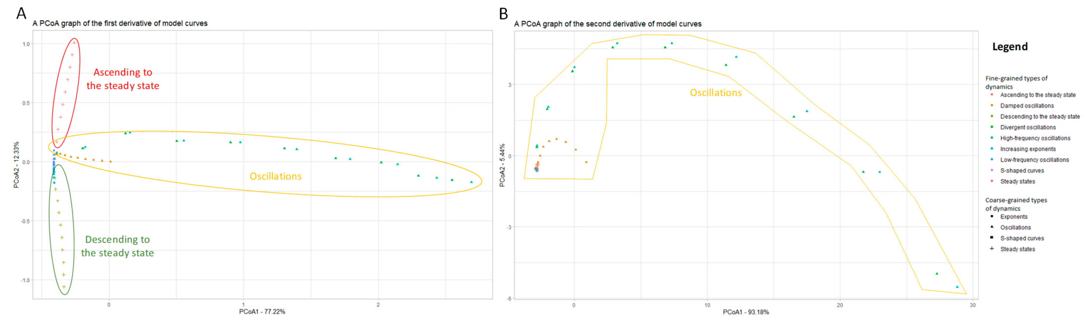
3.1.2. Using Approximations of the Derivatives to Include Additional Information on Curves

Extremes are also an important feature of functions that affect the type of dynamics, so we considered how the approximations of the derivatives of the dynamics in question would be arranged in the principal coordinate space. The central difference was taken to approximate the first derivative:

$$\frac{\partial f_i}{\partial x}\approx \frac{f_{i+1}-f_{i-1}}{2\Delta x}$$

The following graph was obtained approximating the first derivative by the central difference (see Figure 6).

It is evident from Figure 6A that the difference between stationary and oscillatory regimes corresponds to the directions given by the principal coordinates, which can be used as a criterion for such a classification. However, some more complex patterns cannot be traced using this representation.

In addition to extrema in terms of the type of dynamic regime of the function under study, its inflection points also play a role. Accordingly, we have also considered how the time series approximating the second derivatives of the original table-defined functions will be arranged in the principal coordinate space (see Figure 6B).

The approximation of the second derivative can be derived from its definition—the ratio of the increment of the function to the increment of the argument, where the approximation of the first derivative acts as the function. This results in the following formula for approximating the second derivative:

$$\frac{{\partial }^2{f}_i}{\partial x^2}\approx \frac{f_{i+1}-2f_i+f_{i-1}}{\Delta x^2}$$

The second derivative allows us to highlight only different oscillatory regimes. Thus, it is possible to obtain some information about the classification of different dynamical regimes, using finite differences to approximate the derivatives.

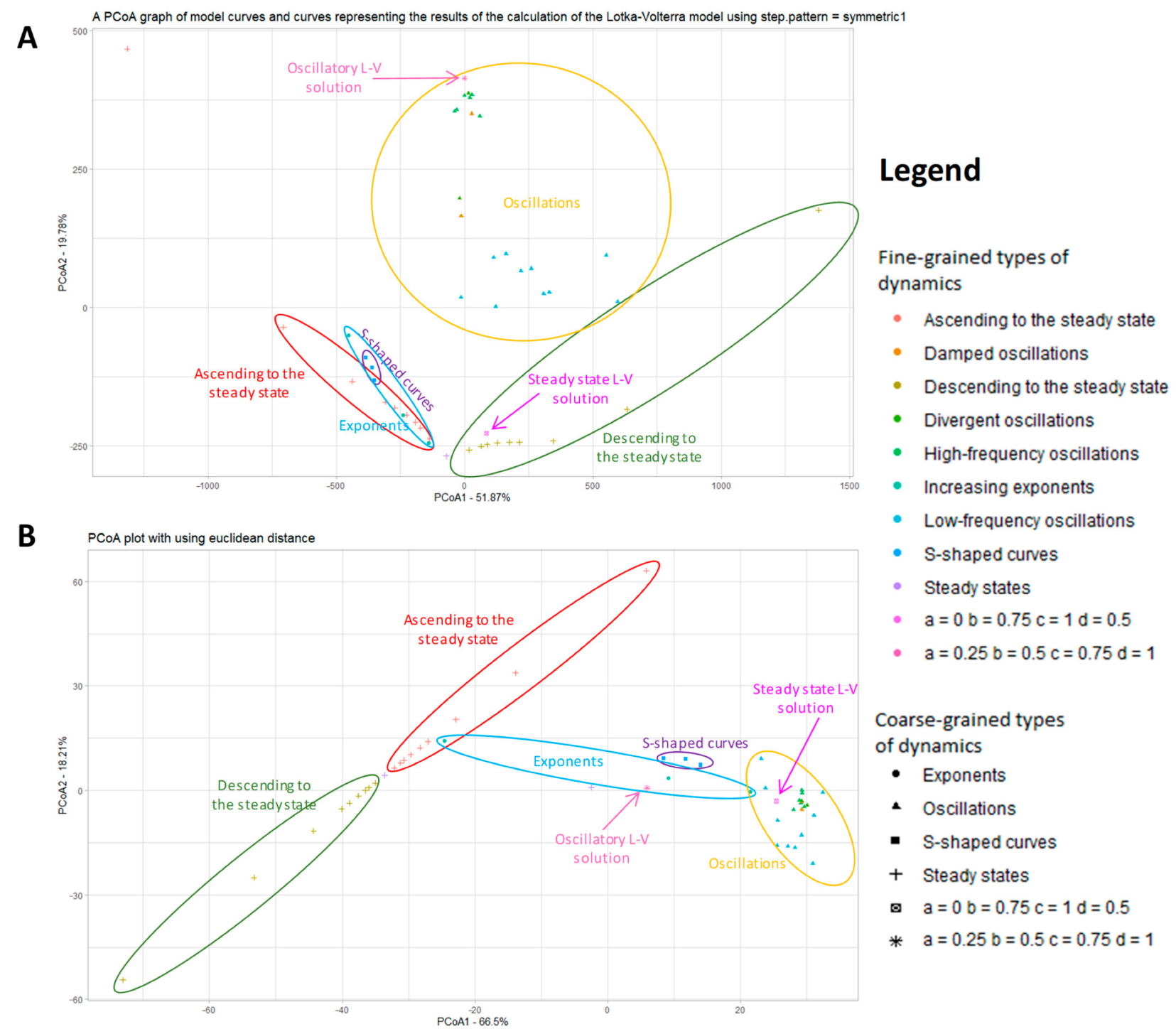
3.1.3. A Comparison with Standard Euclidean Principal Coordinate Analysis

To assess the advantages granted by incorporating dynamic time warping into the principal coordinates analysis (PCoA) we have compared the results with a common PCoA using Euclidean distance. We have also included a steady-state and oscillatory solution of Lotka–Volterra (L-V) model into the analysis of different types of dynamic regimes. The results of the comparison are presented in Figure 7.

Though both approaches work quite well with the artificial set of curves, validation with real L-V solutions shows that dynamic time warping allows putting those into a correct category on a diagram (more diagrams with other step patterns can be found in Supplementary Materials, Figure S2).

Thus, we have demonstrated that our PCoA+DTW approach using symmetric1 step pattern manages to classify the solutions by corresponding types better than standard Euclidean PCoA.

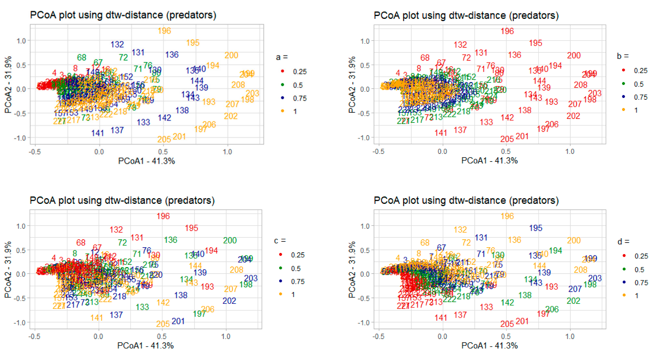
3.2. Parametric Sensitivity Analysis of Dynamical Systems Models: Case Study of the Lotka–Volterra Model

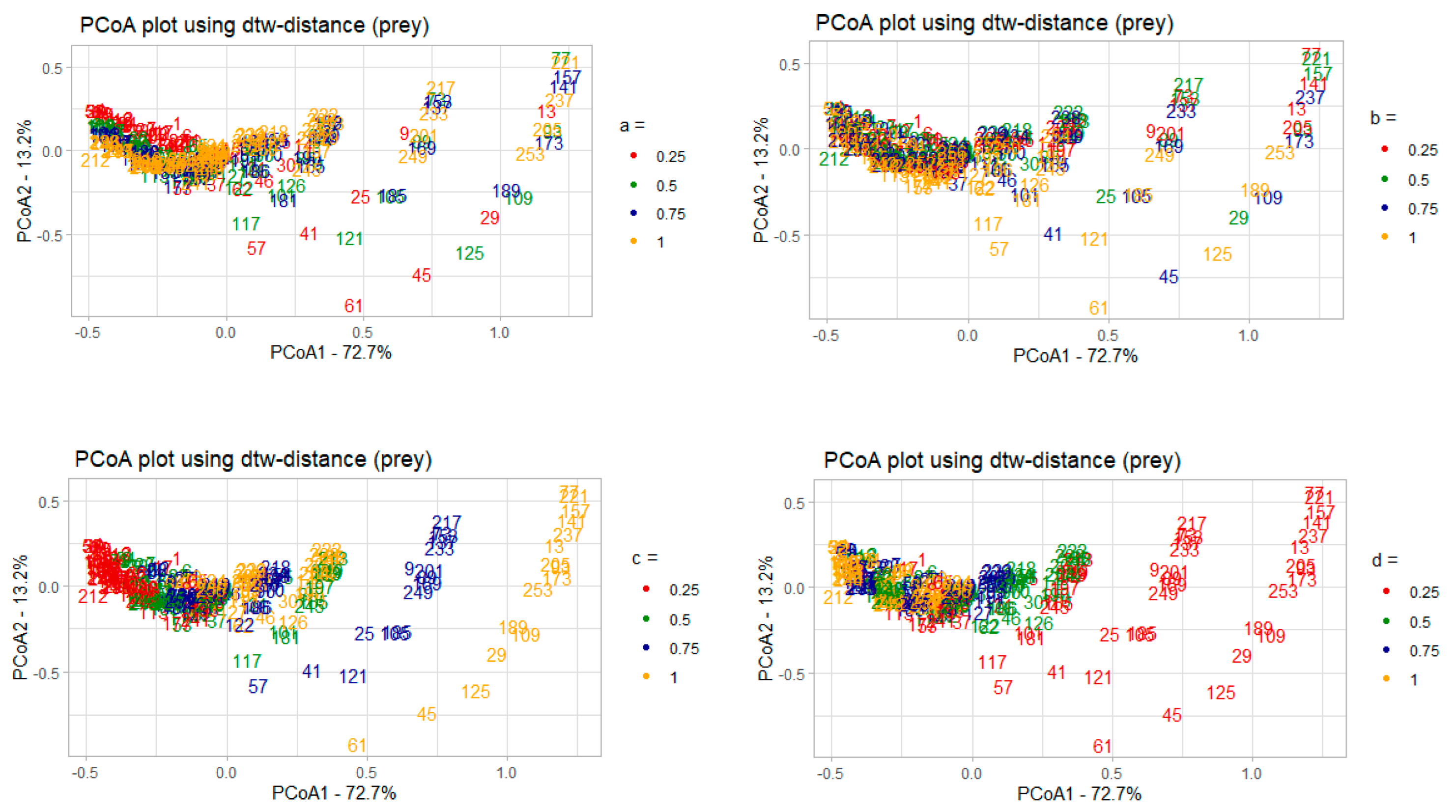
3.2.1. Correlation Analysis of the Model Parameters and PCoA Axes with Respect to the Predator and Prey Populations

The proposed method can also be used to analyze the parametric sensitivity of models of dynamical systems. The well-studied Lotka–Volterra model was chosen as a model to calibrate the developed method of parametric sensitivity analysis [41,42,43], describing the interaction between two populations of the “predator–prey” type. We assume a closed habitat with two species, prey species and predators. We assume that animals do not migrate, and that there is plenty of food for the prey species.

In mathematical form, the proposed system looks as follows:

$$\left\{\begin{array}{c}\frac{dx}{dt}=ax-bxy\\ \frac{dy}{dt}=-cy+dxy\end{array}\right.$$

(9)

This model consists of two ODEs in which x is the density of prey, y is the density of predators, $\frac{dx}{dt}$ is the rate of change in the density of the prey population, and $\frac{dy}{dt}$ is the rate of change in the density of the predators. The model also has four parameters: $a,b,c,d$, which are coefficients reflecting interactions between populations and internal properties of individual populations:

• 𝑎–coefficient of prey growth;
• 𝑏—coefficient of loss of prey caused by interaction with predators;
• 𝑐—coefficient of loss of predators;
• 𝑑—coefficient of predator growth due to interaction with prey species.

This system has two singular points—one point of the “center” type, and one of the “saddle” type. With different initial data in the system, it is possible for only prey to survive, for both species to die out, or for them to coexist. In the latter case, there are usually fluctuations in species numbers, with fluctuations in predator numbers lagging behind fluctuations in prey numbers in the model. There is also a stationary solution, in which both populations are nonzero. Varying the parameter values with fixed initial data also leads to different outcomes from those described above.

Varying the parameters 𝑎, b, 𝑐, 𝑑 from 0.25 to 1 with a step of 0.25, 256 numerical experiments were generated using the Scilab package. The initial conditions in each of the experiments are the same: the prey population density is 5 and the predator population density is 2. The examples of the model solutions at the parameter sets 𝑎 = 0.25, 𝑏 = 0.5, 𝑐 = 0.25, 𝑑 = 0.5 and 𝑎 = 1, 𝑏 = 1, 𝑐 = 1, 𝑑 = 0.25 are shown in Figure S4. The obtained solutions are oscillations with different frequencies and magnitudes (see Figure S4 in Supplementary Materials). The results of the calculations were recorded in the form of time course data, which were used as a sample for further analysis. The average values of frequency and magnitude of oscillations were also calculated for each of the solutions. To obtain the frequencies, it was necessary to find the periods (T) of oscillations through the search of extrema of the function, which is the solution of the model for each individual set of parameters; then, the frequency was calculated as follows: $\nu =1/T$. To find the magnitudes of the solutions, the average values of each of the populations were calculated and then the distances from extrema to these values were calculated. The results are shown in Figure 8 and Figure 9.

Color changes along the first principal coordinate (PCoA1), which is the most informative, can be traced for the parameters c (coefficient of loss of predators) and d (coefficient of growth of predators), which can be interpreted as higher sensitivity of the model to changes in these parameters in relation to the prey population (see Table 1 for Pearson correlation coefficients reflecting the relationship between the parameters and the principal coordinates).

Table 2. Correlation coefficients for each of the model parameters with PCoA1 and PCoA2 with respect to the prey population. Cells with correlation values that did not pass the significance threshold (i.e., those with p-value ≥ 0.05) are marked in gray.

	a	b	C	d
PCoA1	0.14	−0.09	0.62	−0.64
PCoA2	0.03	−0.36	−0.12	0.14

shows that PCoA1 has the greatest dependence with parameters c and d, as the correlation coefficient of these parameters with PCoA1 is the highest by its absolute value. Similar results of analysis based on predator population density data are presented below (see Figure 9).

The situation here is the opposite—the change in colors relative to the first principal coordinate can be traced for the parameters a (coefficient of prey growth) and b (coefficient of loss of prey), indicating that with respect to the dynamics of the predator population, this model is the most sensitive to changes in these parameters.

The analysis of the correlation between the principal coordinates and the model parameters also shows that parameters a and b have the highest correlation with PCoA1 (see

Table 3. Correlation coefficient values of each of the model parameters with PCoA1 and PCoA2 with respect to the predator population. Cells with correlation values that did not pass the significance threshold (i.e., those with p-value ≥ 0.05) are marked in gray.

	a	b	c	d
PCoA1	0.54	−0.59	0.12	0.23
PCoA2	−0.33	−0.05	−0.37	0.59

). We can also note that parameter d correlates quite strongly with PCoA2, which also accounts for a large part of the explained variance.

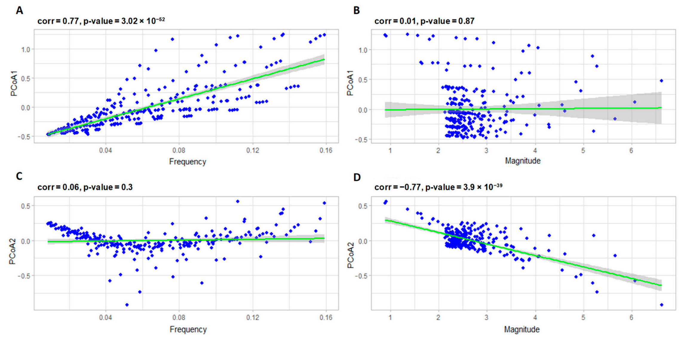
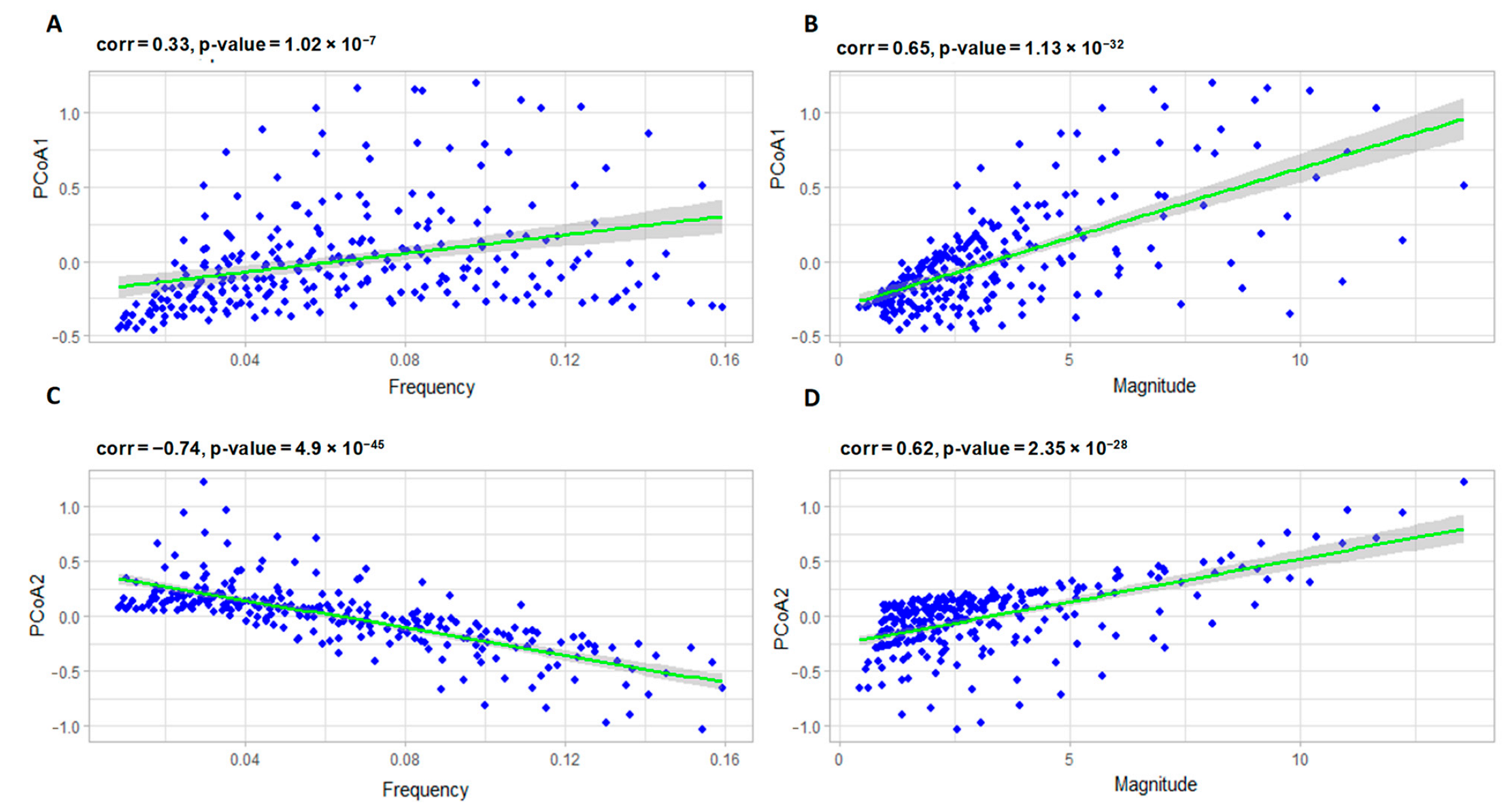
3.2.2. Interpreting PCoA Axes in Terms of Characteristics of Solutions

When using PCoA, which constructs the principal coordinate axes, the method does not directly provide information about what these axes stand for since it only receives a distance matrix as an input. In order to understand the meaning of the principal coordinates, a correlation analysis of these axes with various characteristics of solutions, such as the frequency and magnitude of oscillations, should be carried out. Pearson correlation coefficients were found for these characteristics with the projections of the corresponding solutions on the first two principal coordinates. The results are shown in Figure 10 for prey and in Figure 11 for predators, respectively.

These scatter plots show a strong correlation of PCoA1 with the oscillation frequency, as well as the correlation of PCoA2 with the oscillation magnitude of prey density. That is, in general, PCoA1 can be interpreted as an axis describing the changes in the frequencies of the solutions for the prey population, and PCoA2—as an axis showing the changes in the magnitudes of fluctuations of these solutions.

One can notice that in predators, the situation is the opposite. We see a strong relation of PCoA1 with the magnitude of oscillations, as well as a very strong relation of PCoA2 with the frequency of oscillations and a fairly strong relation with the magnitude. That is, in general, PCoA1 can be interpreted as an axis describing changes in the magnitudes of solutions for predator populations, and PCoA2 as an axis showing changes in both frequencies and magnitudes of predator populations simultaneously.

To assess whether the constructed method is capable of detecting solutions of different types, we added stationary solutions found at zero parameters to the analyzed sample: solution 257 was obtained at c = 0, solution 258 at a = 0, c = 0, solution 259 at a = 0, d = 0, and solution 260 at a = 0. The results obtained show (see Figure S3 in Supplementary Materials) that for the dynamics of the prey population, the method was able to cluster the stationary and oscillatory solutions, but with some inaccuracies (e.g., the 259th point does not lie in the cluster, although it is quite close to it). Consider the projections of predator population dynamics on the principal coordinate axes in the case when there are samples with zero parameters, i.e., stationary solutions. As we can see from Figure S3B, stationary and nonstationary samples did not cluster in this case. The reason lies in the nature of an outlier (the 257th is the Lotka–Volterra model solution with parameters a = 0.5, b = 0.25, c = 0, d = 1). The difference of this solution from others having zero parameters is that it demonstrates the very large magnitude of predator oscillations compared to the solutions 258–260, in which the magnitude of predators is close to zero. That is, for the predator population, the method primarily clusters the data by magnitude rather than by the solution type, and, therefore, should be used with caution.

4. Conclusions

The developed method allows us to obtain a qualitative visualization of the results of the set of solutions of a mathematical model and to carry out the correspondence between the values of the model parameters and the type of dynamic regimes of its solutions. The method can be adjusted by changing the step pattern of the dynamic time warping algorithm; for a better analysis, it can also be applied to the time series approximating the first and second derivatives of the original series. This method was tested on the Lotka–Volterra model and artificial sets of different dynamics. In the course of this work, a new method was proposed for studying the parametric sensitivity of models of dynamical systems on the basis of numerical simulation data. The main difference of the method proposed in this work from the existing methods of studying the parametric sensitivity is that it is universal, not being attached to any particular type of model (in particular, ODE), which allows it to cover a wide class of problems in computational biology and other areas actively using the mathematical modeling of dynamic systems. An important aspect of the proposed method is the use of a black-box approach, which does not imply any additional restrictions on the type of system or even on the formalism in which the model is composed. The only requirement is the ability of the model to generate dynamic trajectories, i.e., time course data, which are the material for all further analysis. The developed method can be used for visualization and classification of various dynamic regimes of models of dynamic systems.

References

1. Boza, G.; Barabás, G.; Scheuring, I.; Zachar, I. Eco-Evolutionary Modelling of Microbial Syntrophy Indicates the Robustness of Cross-Feeding over Cross-Facilitation. Sci. Rep. 2023, 13, 907. [Google Scholar] [CrossRef]
2. Kuntal, B.K.; Gadgil, C.; Mande, S.S. Web-GLV: A Web Based Platform for Lotka-Volterra Based Modeling and Simulation of Microbial Populations. Front. Microbiol. 2019, 10, 288. [Google Scholar] [CrossRef]
3. Krysiak-Baltyn, K.; Martin, G.J.O.; Stickland, A.D.; Scales, P.J.; Gras, S.L. Computational Models of Populations of Bacteria and Lytic Phage. Crit. Rev. Microbiol. 2016, 42, 942–968. [Google Scholar] [CrossRef] [PubMed]
4. Wei, Y.; Wang, X.; Liu, J.; Nememan, I.; Singh, A.H.; Weiss, H.; Levin, B.R. The Population Dynamics of Bacteria in Physically Structured Habitats and the Adaptive Virtue of Random Motility. Proc. Natl. Acad. Sci. USA 2011, 108, 4047–4052. [Google Scholar] [CrossRef] [PubMed] [Green Version]
5. DeAngelis, D.L.; Mooij, W.M. Individual-Based Modeling of Ecological and Evolutionary Processes. Annu. Rev. Ecol. Evol. Syst. 2005, 36, 147–168. [Google Scholar] [CrossRef]
6. Kreft, J.; Picioreanu, C.; Wimpenny, J.W.T.; Loosdrecht, M.C.M. Van. Individual-Based Modelling of Biofilms. Microbiology 2001, 147, 2897–2912. [Google Scholar] [CrossRef] [Green Version]
7. Lardon, L.A.; Merkey, B.V.; Martins, S.; Dötsch, A.; Picioreanu, C.; Kreft, J.U.; Smets, B.F. IDynoMiCS: Next-Generation Individual-Based Modelling of Biofilms. Environ. Microbiol. 2011, 13, 2416–2434. [Google Scholar] [CrossRef]
8. Ayllón, D.; Railsback, S.F.; Vincenzi, S.; Groeneveld, J.; Almodóvar, A.; Grimm, V. InSTREAM-Gen: Modelling Eco-Evolutionary Dynamics of Trout Populations under Anthropogenic Environmental Change. Ecol. Modell. 2016, 326, 36–53. [Google Scholar] [CrossRef]
9. Klimenko, A.; Matushkin, Y.; Kolchanov, N.; Lashin, S. Leave or Stay: Simulating Motility and Fitness of Microorganisms in Dynamic Aquatic Ecosystems. Biology 2021, 10, 1019. [Google Scholar] [CrossRef]
10. Hellweger, F.L.; Clegg, R.J.; Clark, J.R.; Plugge, C.M.; Kreft, J.U. Advancing Microbial Sciences by Individual-Based Modelling. Nat. Rev. Microbiol. 2016, 14, 461–471. [Google Scholar] [CrossRef]
11. Misirli, G.; Nguyen, T.; McLaughlin, J.A.; Vaidyanathan, P.; Jones, T.S.; Densmore, D.; Myers, C.; Wipat, A. A Computational Workflow for the Automated Generation of Models of Genetic Designs. ACS Synth. Biol. 2019, 8, 1548–1559. [Google Scholar] [CrossRef]
12. Shmulevich, I.; Dougherty, E.R.; Kim, S.; Zhang, W. Probabilistic Boolean Networks: A Rule-Based Uncertainty Model for Gene Regulatory Networks. Bioinformatics 2002, 18, 261–274. [Google Scholar] [CrossRef] [Green Version]
13. Wimpenny, J.W.T.; Colasanti, R. A Unifying Hypothesis for the Structure of Microbial Biofilms Based on Cellular Automaton Models. FEMS Microbiol. Ecol. 1997, 22, 1–16. [Google Scholar] [CrossRef]
14. Ashby, B.; Gupta, S.; Buckling, A. Spatial Structure Mitigates Fitness Costs in Host-Parasite Coevolution. Am. Nat. 2014, 183, E64–E74. [Google Scholar] [CrossRef] [PubMed]
15. Thiele, J.C.; Kurth, W.; Grimm, V. Facilitating Parameter Estimation and Sensitivity Analysis of Agent-Based Models: A Cookbook Using NetLogo and R.; University of Surrey: Surrey, UK, 2014; Volume 17, p. 11. [Google Scholar] [CrossRef]
16. Sedlmair, M.; Heinzl, C.; Bruckner, S.; Piringer, H.; Moller, T. Visual Parameter Space Analysis: A Conceptual Framework. IEEE Trans. Vis. Comput. Graph. 2014, 20, 2161–2170. [Google Scholar] [CrossRef] [PubMed]
17. Malik-Sheriff, R.S.; Glont, M.; Nguyen, T.V.N.; Tiwari, K.; Roberts, M.G.; Xavier, A.; Vu, M.T.; Men, J.; Maire, M.; Kananathan, S.; et al. BioModels—15 Years of Sharing Computational Models in Life Science. Nucleic Acids Res. 2019, 48, D407–D415. [Google Scholar] [CrossRef] [Green Version]
18. Olivier, B.G.; Snoep, J.L. Web-Based Kinetic Modelling Using JWS Online. Bioinformatics 2004, 20, 2143–2144. [Google Scholar] [CrossRef] [Green Version]
19. Lloyd, C.M.; Lawson, J.R.; Hunter, P.J.; Nielsen, P.F. The CellML Model Repository. Bioinformatics 2008, 24, 2122–2123. [Google Scholar] [CrossRef] [PubMed]
20. King, Z.A.; Lu, J.; Dräger, A.; Miller, P.; Federowicz, S.; Lerman, J.A.; Ebrahim, A.; Palsson, B.O.; Lewis, N.E. BiGG Models: A Platform for Integrating, Standardizing and Sharing Genome-Scale Models. Nucleic Acids Res. 2016, 44, D515–D522. [Google Scholar] [CrossRef] [PubMed]
21. Colléter, M.; Valls, A.; Guitton, J.; Gascuel, D.; Pauly, D.; Christensen, V. Global Overview of the Applications of the Ecopath with Ecosim Modeling Approach Using the EcoBase Models Repository. Ecol. Model. 2015, 302, 42–53. [Google Scholar] [CrossRef]
22. Hamby, D.M. A Review of Techniques for Parameter Sensitivity Analysis of Environmental Models. Environ. Monit. Assess. 1994, 32, 135–154. [Google Scholar] [CrossRef]
23. Ingalls, B. Sensitivity Analysis: From Model Parameters to System Behaviour. Essays Biochem. 2008, 45, 177–194. [Google Scholar] [CrossRef] [PubMed] [Green Version]
24. Zi, Z. Sensitivity Analysis Approaches Applied to Systems Biology Models. IET Syst. Biol. 2011, 5, 336–346. [Google Scholar] [CrossRef] [PubMed]
25. Zhang, X.Y.; Trame, M.N.; Lesko, L.J.; Schmidt, S. Sobol Sensitivity Analysis: A Tool to Guide the Development and Evaluation of Systems Pharmacology Models. CPT Pharmacomet. Syst. Pharmacol. 2015, 4, 69–79. [Google Scholar] [CrossRef] [PubMed]
26. Saltelli, A.; Homma, T. Importance Measures in Global Sensitivity Analysis of Model Output. Reliab. Eng. Sys. Saf. 1996, 52, 1–17. [Google Scholar]
27. Keogh, E.J.; Pazzani, M.J. Derivative Dynamic Time Warping. In Proceedings of the SIAM International Conference on Data Mining, SDM 2001, Chicago, IL, USA, 5–7 April 2001. [Google Scholar]
28. Giorgino, T. Computing and Visualizing Dynamic Time Warping Alignments in R: The Dtw Package. J. Stat. Softw. 2009, 31, 1–24. [Google Scholar] [CrossRef] [Green Version]
29. Smith, T.F.; Waterman, M.S. Comparison of Biosequences. Adv. Appl. Math. 1981, 2, 482–489. [Google Scholar] [CrossRef] [Green Version]
30. Beijering, K.; Gooskens, C.; Heeringa, W. Predicting Intelligibility and Perceived Linguistic Distance by Means of the Levenshtein Algorithm. Linguist. Neth. 2008, 25, 13–24. [Google Scholar] [CrossRef] [Green Version]
31. Needleman, S.B.; Wunsch, C.D. A General Method Applicable to the Search for Similarities in the Amino Acid Sequence of Two Proteins. J. Mol. Biol. 1970, 48, 443–453. [Google Scholar] [CrossRef]
32. Legendre, P.; Gallagher, E.D. Ecologically Meaningful Transformations for Ordination of Species Data. Oecologia 2001, 129, 271–280. [Google Scholar] [CrossRef]
33. Yang, D.; Dong, Z.; Lim, L.H.I.; Liu, L. Analyzing Big Time Series Data in Solar Engineering Using Features and PCA. Sol. Energy 2017, 153, 317–328. [Google Scholar] [CrossRef] [Green Version]
34. Терехина, А.Ю. Метoды Мнoгoмернoгo Шкалирoвания и Визуализации Данных (Обзoр). Автoмат. и телемех. 1973, 34, 80–94. [Google Scholar]
35. Anderson, M.J.; Willis, T.J. Canonical Analysis of Principal Coordinates: A Useful Method of Constrained Ordination for Ecology. Ecology 2003, 84, 511–525. [Google Scholar] [CrossRef]
36. Groth, D.; Hartmann, S.; Klie, S.; Selbig, J. Principal Components Analysis. Methods Mol. Biol. 2013, 930, 527–547. [Google Scholar] [CrossRef]
37. Gower, J.C. Some Distance Properties of Latent Root and Vector Methods Used in Multivariate Analysis. Biometrika 1966, 53, 325–338. [Google Scholar] [CrossRef]
38. Ramette, A. Multivariate Analyses in Microbial Ecology. FEMS Microbiol. Ecol. 2007, 62, 142–160. [Google Scholar] [CrossRef] [Green Version]
39. Cortopassi, K.A.; Bradbury, J.W. The Comparison of Harmonically Rich Sounds Using Spectrographic Cross-Correlation and Principal Coordinates Analysis. Bioacoustics 2000, 11, 89–127. [Google Scholar] [CrossRef]
40. Jones, M.C.; Rice, J.A. Displaying the Important Features of Large Collections of Similar Curves. Am. Stat. 1992, 46, 140–145. [Google Scholar] [CrossRef]
41. Wangersky, P.J. Lotka-Volterra Population Models Lotka-Volterra*: 4140 Population Models. Source Annu. Rev. Ecol. Syst. Ann. Rev. Ecol. Syst 1978, 9, 189–218. [Google Scholar] [CrossRef]
42. Lotka, A.J. Contribution to the Theory of Periodic Reactions. J. Phys. Chem. 1909, 14, 271–274. [Google Scholar] [CrossRef] [Green Version]
43. Volterra, V. Variazioni e Fluttuazioni Del Numero d’individui in Specie Animali Conviventi; Atti dell’ Accademia Nazionale dei Lincei: Lincei, Italy, 1926; Volume 62, pp. 31–113. [Google Scholar]
Figure 1. (A) Alignment of two time series: noisy sine (red dashed line) and smooth cosine (black continuous line). (B) The warping curve in the case of alignment of two time series: noisy sine and smooth cosine.
Mathematics 11 02783 g001
Figure 2. Warping curves for different step patterns. Warping curve for DTW alignment of noisy sine and smooth cosine (A) using step.pattern = symmetric2; (B) using step.pattern = symmetric1.
Mathematics 11 02783 g002
Figure 3. Computational protocol of analysis and visualization of the results of mass computational experiments based on the pre-calculated set of time dynamics at different sets of parameters.
Mathematics 11 02783 g003
Figure 4. Examples of time series corresponding to different types of dynamic regimes.
Mathematics 11 02783 g004
Figure 5. Location of samples of curves representing different dynamical modes in the space of principal coordinates. The captions to the axes indicate the fractions of the explained variance corresponding to a principal coordinate. Different symbols indicate different types of regimes, and colors indicate subtypes within the types. In calculating the DTW distance, the step pattern (A) symmetric2; (B) symmetric1; (C) asymmetric; (D) rabinerJuang were applied.
Mathematics 11 02783 g005
Figure 6. The result of applying the developed algorithm to the time series approximating (A) the first derivatives of the original series; (B) the second derivatives of the original series. When calculating the DTW distance, the symmetric2 step pattern was applied.
Mathematics 11 02783 g006
Figure 7. The results of PCoA analysis on artificially generated model curves implementing different types of dynamic regimes and Lotka–Volterra model typical solutions (oscillatory and steady-state) using DTW distance with symmetric1 step pattern (A) and common Euclidean distance (B).
Mathematics 11 02783 g007
Figure 8. The model solutions calculated based on the prey densities, with samples colored according to the values of each of the four parameters. The numbers in each of the diagrams correspond to the model solutions for a unique set of parameters from a particular parametric grid. The fractions of the explained variance of the initial sample are given in percent.
Mathematics 11 02783 g008
Figure 9. The model solutions calculated based on the predator densities, with samples colored according to the values of each of the four parameters. The numbers in each of the diagrams correspond to the model solutions for a unique set of parameters from a particular parametric grid. The fractions of the explained variance of the initial sample are given in percent.
Mathematics 11 02783 g009
Figure 10. Results of correlation analysis of the oscillation frequency of prey and PCoA1 (A), the oscillation magnitude of prey and PCoA1 (B), the oscillation frequency of prey and PCoA2 (C), and the oscillation magnitude of prey and PCoA2 (D).
Mathematics 11 02783 g010
Figure 11. Results of correlation analysis of the oscillation frequency of predator and PCoA1. (A) The oscillation magnitude of predator and PCoA1, (B) the oscillation frequency of predator and PCoA2, (C) and the oscillation magnitude of predator and PCoA2 (D).
Mathematics 11 02783 g011