

Magnetohydrodynamics Williamson Nanofluid Flow over an Exponentially Stretching Surface with a Chemical Reaction and Thermal Radiation

Abstract
1. Introduction
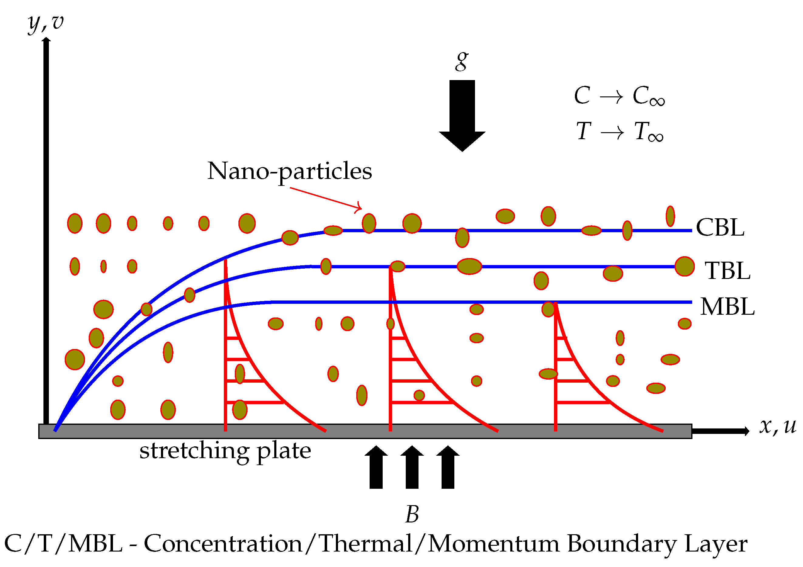
2. Fluid Model
3. Mathematical Analysis
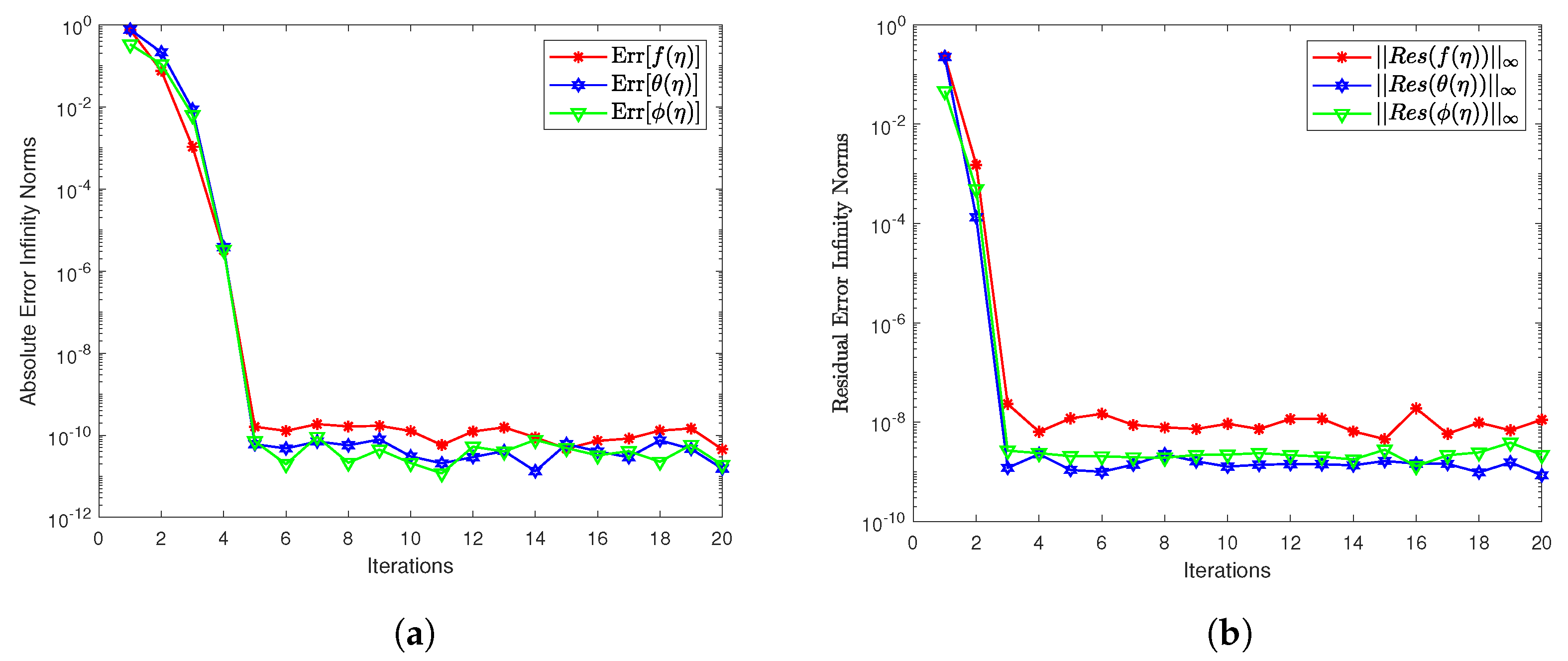
4. Method of Solution
- , ,
- ,
- .
5. Results and Discussion
5.1. Validation of Results
- sol = bvp4c(@odeBVP, @odeBc, solinit, options).
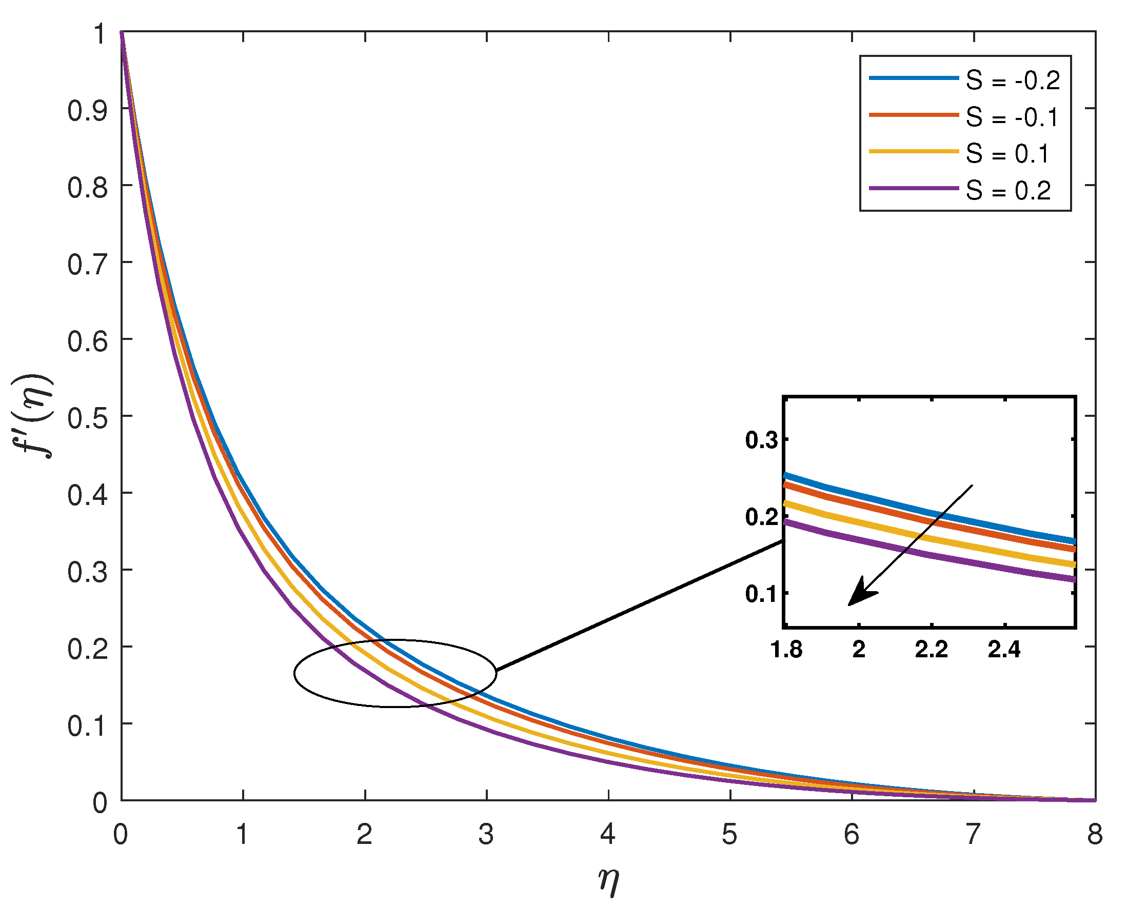
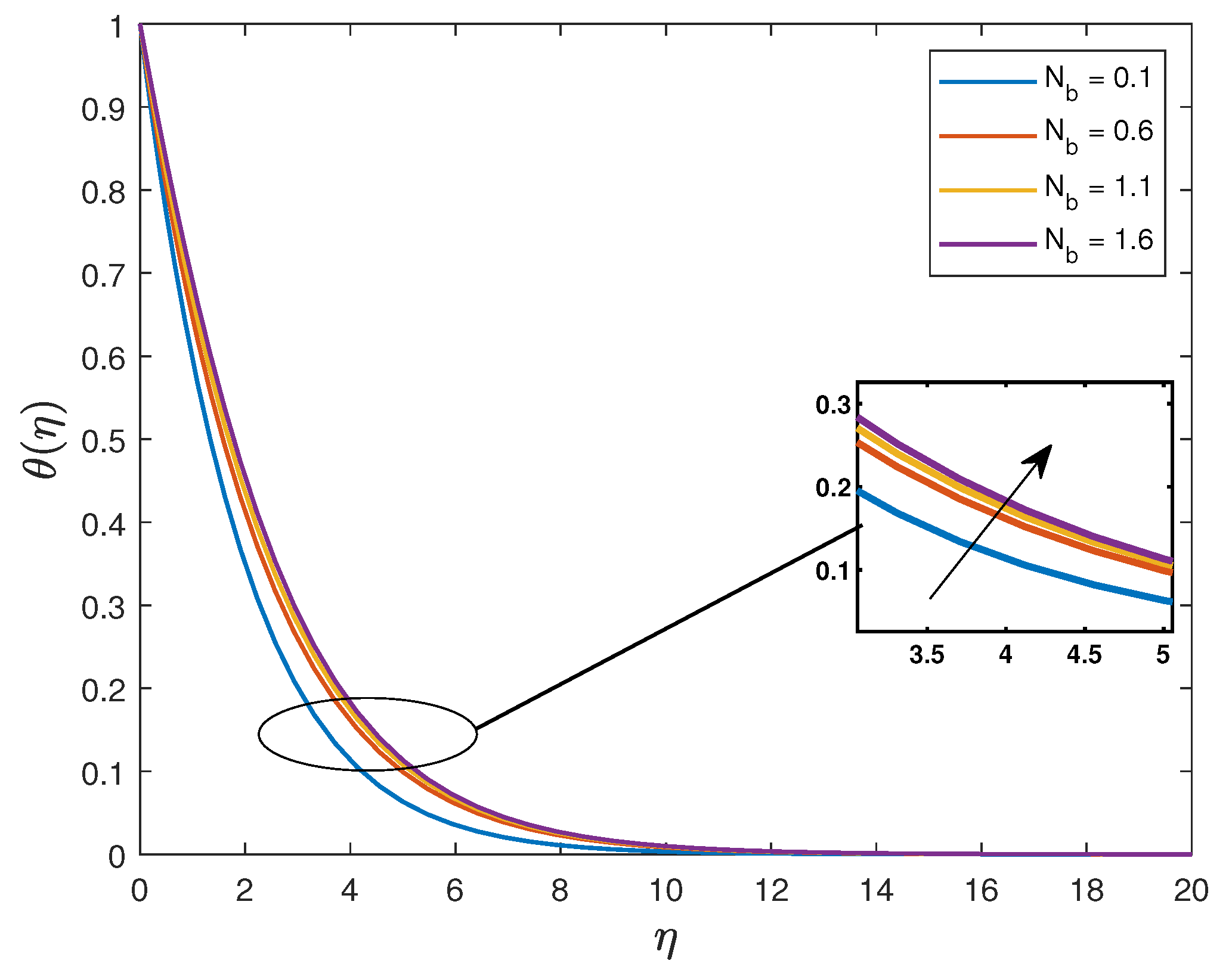
5.2. Results
6. Conclusions
- The dimensionless velocity diminishes as the values of the magnetic parameter are increased from 0 to ;
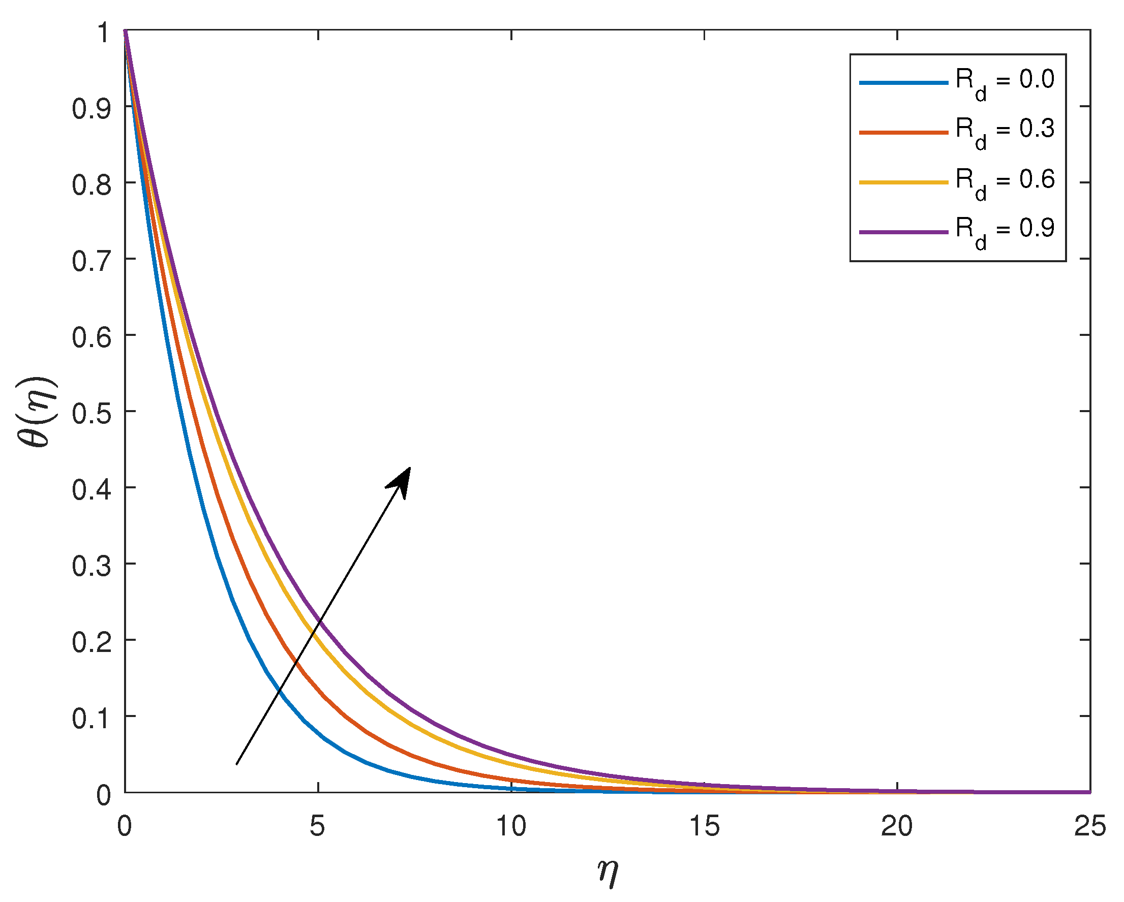
- The dimensionless temperature is an increasing function of and ;
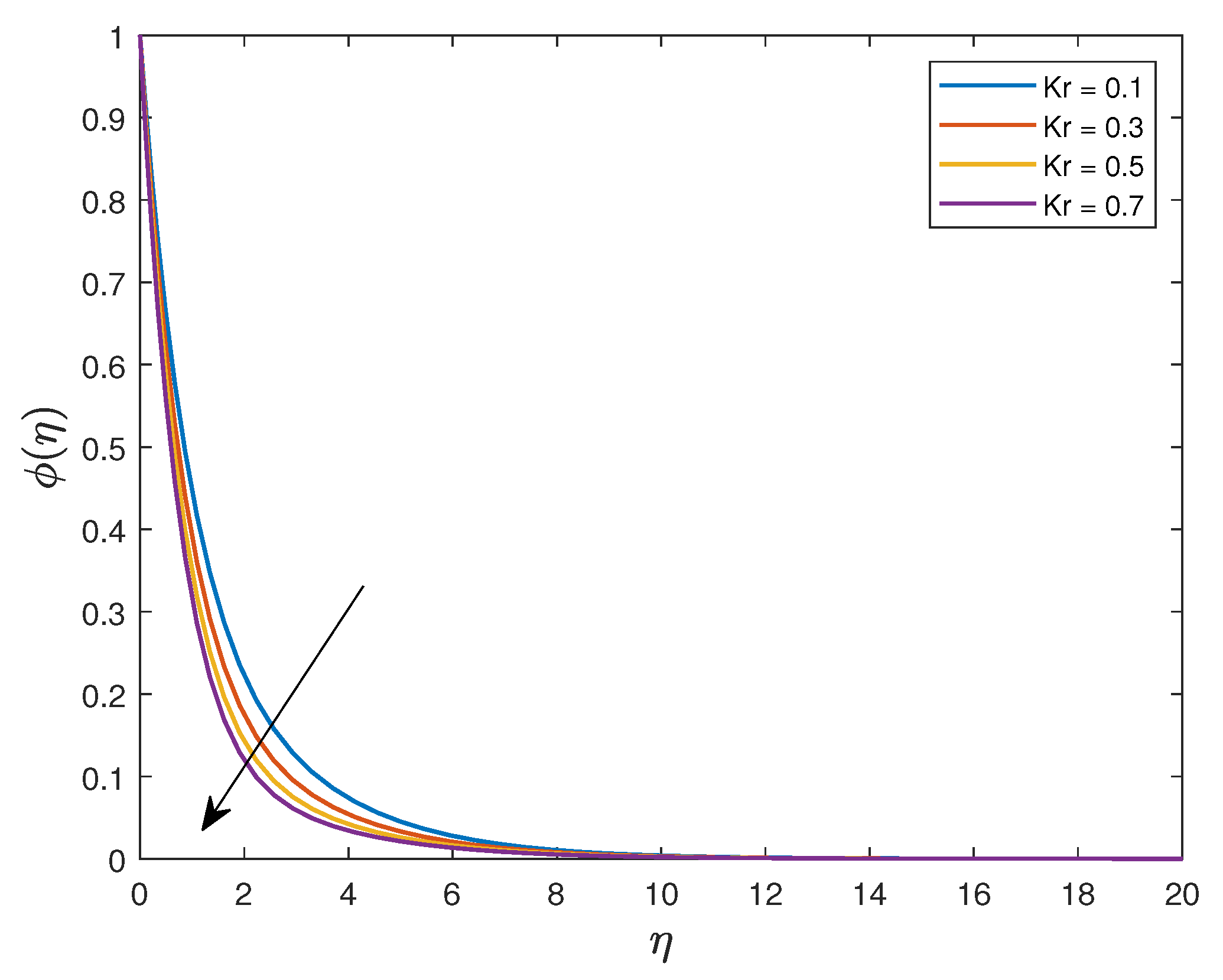
- The dimensionless concentration decreases for and ;
- The skin friction coefficient increases as and increase and depressed for increased values of ;
- The Nusselt number diminishes as , and are increased;
- The Sherwood number decreases as and increase and decreases as increases.
Author Contributions
Funding
Data Availability Statement
Conflicts of Interest
Nomenclature
| Cartesian coordinates [m] | |
| Velocity components in the x and y directions, respectively [m s] | |
| Reference velocity [m s] | |
| Thermal expansion coefficient | |
| Concentration expansion coefficient | |
| Magnetic field strength [NmA] | |
| Skin friction coefficient | |
| Prandtl number | |
| M | Magnetic parameter [Te] |
| T | Fluid temperature [T] |
| Concentration of nanoparticles at the surface [mol m] | |
| C | Concentration of nanoparticles [mol m] |
| Velocity at the wall [m s] | |
| Q | Heat source |
| Chemical reaction parameter [Ms] | |
| Reference temperature [K] | |
| Reference concentration [mol m] | |
| Thermal radiation parameter | |
| Radiative heat flux [J] | |
| S | Suction/injection parameter |
| Dimensionless temperature | |
| Dimensionless concentration | |
| Thermophoretic parameter | |
| Local Nusselt number | |
| Local Sherwood number | |
| Surface temperature [K] | |
| Ambient temperature [K] | |
| f | Dimensionless stream function |
| g | Acceleration due to gravity [m s] |
| Schmidt number | |
| Brownian diffusion coefficient [m s] | |
| Thermophoresis diffusion coefficient [m s] | |
| Infinite viscosity [Nsm] | |
| Heat capacity of the nanofluid [JmK] | |
| Reynolds number | |
| Velocity profile | |
| Dimensionless similarity variable | |
| Electrical conductivity [Sm] | |
| Positive time constant | |
| Thermal diffusivity [m s] | |
| Heat capacity of the nanoparticles [Jm K] | |
| Kinematic viscosity [m s] | |
| Fluid density [kg m] | |
| Williamson fluid parameter | |
| Thermal Grashof number | |
| Concentration Grashof number |
References
- Matsuhisa, S.; Bird, R.B. Analytical and numerical solutions for laminar flow of the non-Newtonian ellis fluid. AIChE J. 1965, 11, 588–595. [Google Scholar] [CrossRef]
- Carreau, P.J. Rheological Equations from Molecular Network Theories. Trans. Soc. Rheol. 1972, 16, 99–127. [Google Scholar] [CrossRef]
- Ostwald, W. Ueber die rechnerische Darstellung des Strukturgebietes der Viskosität. Kolloid Z. 1929, 47, 176–187. [Google Scholar] [CrossRef]
- Cross, M.M. Rheology of non-Newtonian fluids: A new flow equation for pseudoplastic systems. J. Colloid Sci. 1965, 20, 417–437. [Google Scholar] [CrossRef]
- Casson, N. A Flow Equation for Pigment-Oil Suspensions of the Printing Ink Type. In Rheology of Disperse Systems; Mill, C.C., Ed.; Pergamon Press: Oxford, UK, 1959; pp. 84–104. [Google Scholar]
- Williamson, R.V. The Flow of Pseudoplastic Materials. Ind. Eng. Chem. 1929, 21, 1108–1111. [Google Scholar] [CrossRef]
- Sakiadis, B.C. Boundary-layer behavior on continuous solid surfaces: I. Boundary-layer equations for two-dimensional and axisymmetric flow. AIChE J. 1961, 7, 26–28. [Google Scholar] [CrossRef]
- Crane, L.J. Flow past a stretching plate. Z. Angew. Math. Phys. ZAMP 1970, 21, 645–647. [Google Scholar] [CrossRef]
- Khan, S.; Selim, M.M.; Khan, A.; Ullah, A.; Abdeljawad, T.; Ikramullah; Ayaz, M.; Mashwani, W.K. On the Analysis of the Non-Newtonian Fluid Flow Past a Stretching/Shrinking Permeable Surface with Heat and Mass Transfer. Coatings 2021, 11, 566. [Google Scholar] [CrossRef]
- Zeb, H.; Bhatti, S.; Khan, U.; Wahab, H.A.; Mohamed, A.; Khan, I. Impact of Homogeneous-Heterogeneous Reactions on Flow of Non-Newtonian Ferrofluid over a Stretching Sheet. J. Nanomater. 2022, 2022, 2501263. [Google Scholar] [CrossRef]
- Mahabaleshwar, U.S.; Maranna, T.; Sofos, F. Analytical investigation of an incompressible viscous laminar Casson fluid flow past a stretching/shrinking sheet. Sci. Rep. 2022, 12, 18404. [Google Scholar] [CrossRef]
- Abbas, N.; Nadeem, S.; Shatanawi, W. Effects of radiation and heat generation for non-Newtonian fluid flow over slendering stretching sheet: Numerically. J. Appl. Math. Mech. 2022, 103, e202100299. [Google Scholar] [CrossRef]
- Akbar, N.S.; Al-Zubaidi, A.; Saleem, S.; Alsallami, S.A.M. Variable fluid properties analysis for thermally laminated 3-dimensional magnetohydrodynamic non-Newtonian nanofluid over a stretching sheet. Sci. Rep. 2023, 13, 3231. [Google Scholar] [CrossRef]
- Masuda, H.; Ebata, A.; Teramae, K.; Hishinuma, N. Alteration of Thermal Conductivity and Viscosity of Liquid by Dispersing Ultra-Fine Particles. Dispersion of Al2O3, SiO2 and TiO2 Ultra-Fine Particles. Netsu Bussei 1993, 7, 227–233. [Google Scholar] [CrossRef]
- Choi, S.U.S.; Eastman, J.A. Enhancing thermal conductivity of fluids with nanoparticle. In Proceedings of the 1995 International Mechanical Engineering Congress and Exhibition, San Francisco, CA, USA, 12–17 November 1995. [Google Scholar]
- Elboughdiri, N.; Ghernaout, D.; Muhammad, T.; Alshehri, A.; Sadat, R.; Ali, M.R.; Wakif, A. Towards a novel EMHD dissipative stagnation point flow model for radiating copper-based ethylene glycol nanofluids: An unsteady two-dimensional homogeneous second-grade flow case study. Case Stud. Therm. Eng. 2023, 45, 102914. [Google Scholar] [CrossRef]
- Ashraf, M.Z.; Rehman, S.U.; Farid, S.; Hussein, A.K.; Ali, B.; Shah, N.A.; Weera, W. Insight into Significance of Bioconvection on MHD Tangent Hyperbolic Nanofluid Flow of Irregular Thickness across a Slender Elastic Surface. Mathematics 2022, 10, 2592. [Google Scholar] [CrossRef]
- Nabwey, H.A.; Rahbar, F.; Armaghani, T.; Rashad, A.M.; Chamkha, A.J. A Comprehensive Review of Non-Newtonian Nanofluid Heat Transfer. Symmetry 2023, 15, 362. [Google Scholar] [CrossRef]
- Selimefendigil, F.; Şenol, G.; Öztop, H.F.; Abu-Hamdeh, N.H. A Review on Non-Newtonian Nanofluid Applications for Convection in Cavities under Magnetic Field. Symmetry 2022, 15, 41. [Google Scholar] [CrossRef]
- Lou, Q.; Ali, B.; Rehman, S.U.; Habib, D.; Abdal, S.; Shah, N.A.; Chung, J.D. Micropolar Dusty Fluid: Coriolis Force Effects on Dynamics of MHD Rotating Fluid When Lorentz Force Is Significant. Mathematics 2022, 10, 2630. [Google Scholar] [CrossRef]
- Alfven, H. Existence of Electromagnetic-Hydrodynamic Waves. Nature 1942, 150, 405–406. [Google Scholar] [CrossRef]
- Abbas, A.; Jeelani, M.B.; Alnahdi, A.S.; Ilyas, A. MHD Williamson Nanofluid Fluid Flow and Heat Transfer Past a Non-Linear Stretching Sheet Implanted in a Porous Medium: Effects of Heat Generation and Viscous Dissipation. Processes 2022, 10, 1221. [Google Scholar] [CrossRef]
- Reddy C, S.; Naikoti, K.; Rashidi, M.M. MHD flow and heat transfer characteristics of Williamson nanofluid over a stretching sheet with variable thickness and variable thermal conductivity. Trans. A. Razmadze Math. Inst. 2017, 171, 195–211. [Google Scholar] [CrossRef]
- Shawky, H.M.; Eldabe, N.T.M.; Kamel, K.A.; Abd-Aziz, E.A. MHD flow with heat and mass transfer of Williamson nanofluid over stretching sheet through porous medium. Microsyst. Technol. 2019, 25, 1155–1169. [Google Scholar] [CrossRef]
- Bouslimi, J.; Omri, M.; Mohamed, R.A.; Mahmoud, K.H.; Abo-Dahab, S.M.; Soliman, M.S. MHD Williamson nanofluid flow over a stretching sheet through a porous medium under effects of joule heating, nonlinear thermal radiation, heat generation/absorption, and chemical reaction. Adv. Math. Phys. 2021, 2021, 9950993. [Google Scholar] [CrossRef]
- Hayat, T.; Bashir, G.; Waqas, M.; Alsaedi, A. MHD 2D flow of Williamson nanofluid over a nonlinear variable thicked surface with melting heat transfer. J. Mol. Liq. 2016, 223, 836–844. [Google Scholar] [CrossRef]
- Ibrahim, W.; Negera, M. The Investigation of MHD Williamson Nanofluid over Stretching Cylinder with the Effect of Activation Energy. Adv. Math. Phys. 2020, 2020, 9523630. [Google Scholar] [CrossRef]
- Eswara Rao, M.; Siva Sankari, M.; Nagalakshmi, C.; Rajkumar, S. On the Role of Bioconvection and Activation Energy for MHD-Stretched Flow of Williamson and Casson Nanofluid Transportation across a Porous Medium Past a Permeable Sheet. J. Nanomater. 2023, 2023, 3995808. [Google Scholar] [CrossRef]
- Asjad, M.I.; Zahid, M.; Ali, B.; Jarad, F. Unsteady MHD Williamson Fluid Flow with the Effect of Bioconvection over Permeable Stretching Sheet. Math. Probl. Eng. 2022, 2022, 7980267. [Google Scholar] [CrossRef]
- Wang, F.; Asjad, M.I.; Rehman, S.U.; Ali, B.; Hussain, S.; Gia, T.N.; Muhammad, T. MHD Williamson Nanofluid Flow over a Slender Elastic Sheet of Irregular Thickness in the Presence of Bioconvection. Nanomaterials 2021, 11, 2297. [Google Scholar] [CrossRef]
- Ahmed, K.; Akbar, T.; Muhammad, T.; Alghamdi, M. Heat transfer characteristics of MHD flow of Williamson nanofluid over an exponential permeable stretching curved surface with variable thermal conductivity. Case Stud. Therm. Eng. 2021, 28, 101544. [Google Scholar] [CrossRef]
- Patil, V.S.; Humane, P.P.; Patil, A.B. MHD Williamson nanofluid flow past a permeable stretching sheet with thermal radiation and chemical reaction. Int. J. Model. Simul. 2023, 43, 185–199. [Google Scholar] [CrossRef]
- Khan, M.; Malik, M.Y.; Salahuddin, T.; Hussian, A. Heat and mass transfer of Williamson nanofluid flow yield by an inclined Lorentz force over a nonlinear stretching sheet. Results Phys. 2018, 8, 862–868. [Google Scholar] [CrossRef]
- Kumar, P.B.S.; Gireesha, B.J.; Gorla, R.S.R.; Mahanthesh, B. Magnetohydrodynamic Flow of Williamson Nanofluid Due to an Exponentially Stretching Surface in the Presence of Thermal Radiation and Chemical Reaction. J. Nanofluids 2017, 6, 264–272. [Google Scholar] [CrossRef]
- Nadeem, S.; Hussain, S.T.; Lee, C. Flow of a Williamson fluid over a stretching sheet. Braz. J. Chem. Eng. 2013, 30, 619–625. [Google Scholar] [CrossRef]
- Ahmed, K.; Akbar, T. Numerical investigation of magnetohydrodynamics Williamson nanofluid flow over an exponentially stretching surface. Adv. Mech. Eng. 2021, 13, 168781402110198. [Google Scholar] [CrossRef]
- Amjad, M.; Ahmed, I.; Ahmed, K.; Alqarni, M.S.; Akbar, T.; Muhammad, T. Numerical Solution of Magnetized Williamson Nanofluid Flow over an Exponentially Stretching Permeable Surface with Temperature Dependent Viscosity and Thermal Conductivity. Nanomaterials 2022, 12, 3661. [Google Scholar] [CrossRef]
- Li, Y.-X.; Alshbool, M.H.; Lv, Y.-P.; Khan, I.; Riaz Khan, M.; Issakhov, A. Heat and mass transfer in MHD Williamson nanofluid flow over an exponentially porous stretching surface. Case Stud. Therm. Eng. 2021, 26, 100975. [Google Scholar] [CrossRef]
- Motsa, S.S.; Dlamini, P.G.; Khumalo, M. Spectral Relaxation Method and Spectral Quasilinearization Method for Solving Unsteady Boundary Layer Flow Problems. Adv. Math. Phys. 2014, 2014, 341964. [Google Scholar] [CrossRef]
- Nadeem, S.; Hussain, S.T. Heat transfer analysis of Williamson fluid over exponentially stretching surface. Appl. Math. Mech. 2014, 35, 489–502. [Google Scholar] [CrossRef]
- Dapra, I.; Scarpi, G. Perturbation solution for pulsatile flow of a non-Newtonian Williamson fluid in a rock fracture. Int. J. Rock Mech. Min. Sci. 2007, 44, 271–278. [Google Scholar] [CrossRef]
- Rosseland, S. Theoretical Astrophysics; Oxford University Press: Oxford, UK, 1936. [Google Scholar]
- Seini, Y.I.; Makinde, O.D. MHD Boundary Layer Flow due to Exponential Stretching Surface with Radiation and Chemical Reaction. Math. Probl. Eng. 2013, 2013, 163614. [Google Scholar] [CrossRef]
- Bellman, R.; Kalaba, R. Quasilinearization and Nonlinear Boundary-Value Problems; American Elsevier Publishing Company: New York, NY, USA, 1965. [Google Scholar]
- Amjad, M.; Ahmed, K.; Akbar, T.; Muhammad, T.; Ahmed, I.; Alshomrani, A.S. Numerical investigation of double diffusion heat flux model in Williamson nanofluid over an exponentially stretching surface with variable thermal conductivity. Case Stud. Therm. Eng. 2022, 36, 102231. [Google Scholar] [CrossRef]
- Motsa, S. On the New Bivariate Local Linearisation Method for Solving Coupled Partial Differential Equations in Some Applications of Unsteady Fluid Flows with Heat and Mass Transfer. In Mass Transfer—Advancement in Process Modelling; InTech: Vienna, Austria, 2015. [Google Scholar] [CrossRef]
- Alharbey, R.A.; Mondal, H.; Behl, R. Spectral Quasi-Linearization Method for Non-Darcy Porous Medium with Convective Boundary Condition. Entropy 2019, 21, 838. [Google Scholar] [CrossRef]


| S | M | Amjad et al. [45] | SQLM | |
|---|---|---|---|---|
| 0.1 | 0.2 | 2.0 | 1.754213 | 1.754213105760364 |
| 0.2 | 0.2 | 2.0 | 1.678675 | 1.678675073146794 |
| 0.3 | 0.2 | 2.0 | 1.579827 | 1.578533717157394 |
| 0.1 | 0.1 | 2.0 | 1.799249 | 1.799249869955796 |
| 0.1 | 0.2 | 2.0 | 1.754213 | 1.754213105760364 |
| 0.1 | 0.3 | 2.0 | 1.710489 | 1.710489423953702 |
| 0.1 | 0.2 | 0.1 | 1.201556 | 1.201559983439274 |
| 0.1 | 0.2 | 0.2 | 1.237223 | 1.237224345281889 |
| 0.1 | 0.2 | 0.3 | 1.271816 | 1.271816653083256 |
| Nadeem and Hussain [40] | MATLAB’s bvp4c | SQLM | |
|---|---|---|---|
| 0.0 | 1.32930 | 1.329302736062721 | 1.329308462412963 |
| 0.1 | 1.29801 | 1.298017071294807 | 1.298022829158239 |
| 0.2 | 1.26310 | 1.263103796098337 | 1.263109548733657 |
| 0.3 | 1.22276 | 1.222776617114427 | 1.222781418705920 |
| S | M | Pr | Sc | Kr | ||||||||||
|---|---|---|---|---|---|---|---|---|---|---|---|---|---|---|
| 0.1 | 0.2 | 2.0 | 0.5 | 0.1 | 0.1 | 0.1 | 0.5 | 0.5 | 0.1 | 1.0 | 0.1 | 1.776767 | 0.308282 | 0.700530 |
| 0.3 | 1.706494 | 0.295463 | 0.687057 | |||||||||||
| 0.9 | 1.608996 | 0.169515 | 0.539204 | |||||||||||
| 0.1 | 0.1 | 1.730004 | 0.323907 | 0.736618 | ||||||||||
| 0.2 | 1.776768 | 0.308282 | 0.700530 | |||||||||||
| 0.3 | 1.824988 | 0.294009 | 0.665454 | |||||||||||
| 0.2 | 0.1 | 1.174219 | 0.434167 | 0.794308 | ||||||||||
| 0.2 | 1.213171 | 0.426083 | 0.787275 | |||||||||||
| 0.3 | 1.251027 | 0.418169 | 0.780543 | |||||||||||
| 2.0 | 0.1 | 1.771939 | 0.147223 | 0.810761 | ||||||||||
| 0.2 | 1.773217 | 0.191519 | 0.780377 | |||||||||||
| 0.3 | 1.774461 | 0.233031 | 0.751949 | |||||||||||
| 0.5 | 0.3 | 1.635586 | 0.347227 | 0.724385 | ||||||||||
| 0.6 | 1.430563 | 0.391337 | 0.757335 | |||||||||||
| 0.9 | 1.232356 | 0.424697 | 0.786362 | |||||||||||
| 0.1 | 0.3 | 1.474263 | 0.368464 | 0.735159 | ||||||||||
| 0.6 | 1.246002 | 0.419482 | 0.777179 | |||||||||||
| 0.9 | 1.027907 | 0.454621 | 0.811112 | |||||||||||
| 0.1 | 0.3 | 1.470957 | 0.273691 | 0.724148 | ||||||||||
| 0.5 | 1.468421 | 0.248889 | 0.741101 | |||||||||||
| 0.7 | 1.466412 | 0.230255 | 0.753849 | |||||||||||
| 0.1 | 0.1 | 1.390481 | 0.316343 | 0.032976 | ||||||||||
| 0.3 | 1.461652 | 0.312301 | 0.593189 | |||||||||||
| 0.5 | 1.474263 | 0.308282 | 0.700530 | |||||||||||
| 0.5 | 0.1 | 1.491310 | 0.358320 | 0.807764 | ||||||||||
| 0.3 | 1.482646 | 0.324544 | 0.753061 | |||||||||||
| 0.5 | 1.474263 | 0.308282 | 0.700530 | |||||||||||
| 0.1 | 0.0 | 1.477366 | 0.382548 | 0.658192 | ||||||||||
| 0.1 | 1.474263 | 0.308282 | 0.700530 | |||||||||||
| 0.2 | 1.470240 | 0.198753 | 0.756672 | |||||||||||
| 0.1 | 0.6 | 1.446575 | 0.322304 | 0.458305 | ||||||||||
| 0.8 | 1.461864 | 0.314201 | 0.587691 | |||||||||||
| 1.0 | 1.474263 | 0.308282 | 0.700530 | |||||||||||
| 1.0 | 0.2 | 1.479727 | 0.303787 | 0.778334 | ||||||||||
| 0.4 | 1.488552 | 0.297958 | 0.906974 | |||||||||||
| 0.6 | 1.495533 | 0.294169 | 1.015232 |
Disclaimer/Publisher’s Note: The statements, opinions and data contained in all publications are solely those of the individual author(s) and contributor(s) and not of MDPI and/or the editor(s). MDPI and/or the editor(s) disclaim responsibility for any injury to people or property resulting from any ideas, methods, instructions or products referred to in the content. |
© 2023 by the authors. Licensee MDPI, Basel, Switzerland. This article is an open access article distributed under the terms and conditions of the Creative Commons Attribution (CC BY) license (https://creativecommons.org/licenses/by/4.0/).
Share and Cite
Muzara, H.; Shateyi, S. Magnetohydrodynamics Williamson Nanofluid Flow over an Exponentially Stretching Surface with a Chemical Reaction and Thermal Radiation. Mathematics 2023, 11, 2740. https://doi.org/10.3390/math11122740
Muzara H, Shateyi S. Magnetohydrodynamics Williamson Nanofluid Flow over an Exponentially Stretching Surface with a Chemical Reaction and Thermal Radiation. Mathematics. 2023; 11(12):2740. https://doi.org/10.3390/math11122740
Chicago/Turabian StyleMuzara, Hillary, and Stanford Shateyi. 2023. "Magnetohydrodynamics Williamson Nanofluid Flow over an Exponentially Stretching Surface with a Chemical Reaction and Thermal Radiation" Mathematics 11, no. 12: 2740. https://doi.org/10.3390/math11122740
APA StyleMuzara, H., & Shateyi, S. (2023). Magnetohydrodynamics Williamson Nanofluid Flow over an Exponentially Stretching Surface with a Chemical Reaction and Thermal Radiation. Mathematics, 11(12), 2740. https://doi.org/10.3390/math11122740