Pricing Variance Swaps under MRG Model with Regime-Switching: Discrete Observations Case

Abstract

In this paper, we creatively price the discretely sampled variance swaps under the mean-reverting Gaussian model (MRG model in short) with regime-switching asymmetric double exponential jump diffusion. We extend the traditional MRG model by further considering the trend of the financial market as well as a sudden and unexpected event of the market. This new model is meaningful because it uses observable Markov chains that represent market states to adjust its parameters, which helps capture the movement of the market and fluctuations in asset prices. By utilizing the characteristic function and the conditional transition characteristic function, we obtain analytical solutions for pricing formulae. Note that this is our first effort to provide the analytical solution for the ordinary differential equations satisfied by the Feynman–Kac theorem. To achieve this, we have developed a new methodology in Proposition 2 that involves dividing the sampling interval into more detailed switching and non-switching intervals. One significant advantage of our closed-form solution is its high computational accuracy and efficiency. Subsequent semi-Monte Carlo simulations will provide specific validation results.

1. Introduction

With the globalization of economies and intensifying competition in financial markets, more and more investors and scholars have realized the importance of hedging against volatility risk. Against this background, volatility derivatives have emerged as instruments that hedge against this volatility risk. Their most prominent feature is that they provide direct exposure to asset volatility without continuous delta-hedging [1]. Among the various volatility derivatives, variance or volatility swaps are considered the main and essential ones. Essentially, they are forward contracts for future realized volatility or variance. The long position of a volatility or variance swap pays a fixed delivery price at expiry and receives the floating amounts of annualized realized volatility or variance, whereas the short position is just the opposite [2]. In other words, the payoff of a variance swap at maturity T is $\left(v^2\left(T\right)-K\right)\times I$, where $v^2\left(T\right)$ is the realized annual variance of the return, K is the strike price such that the initial value of the variance swap equal to zero for both long and short positions, and I is the notional amount of the swap in dollars per annualized volatility point squared.

In the literature, there are roughly two types of approaches for pricing volatility swaps or variance swaps: static replication methods and model-based stochastic methods. Static replication means that a variance swap could be replicated theoretically by using a portfolio of standard options and without specifying the volatility function. For example, Demeterfi [1] produced some of the most influential pioneering work that demonstrated how to use a standard option portfolio to replicate variance swaps. Obviously, the outstanding advantage of static replication is that it does not require a specific model to solve pricing problems [3], and this method has been widely used for the VIX index since 2003 [4]. However, according to Sahalia et al. [5], this method has drawbacks that make it unsuitable for the real market. These include the inability to promptly reflect jumping variance swap rates, as well as the need for constant adjustment in options. Therefore, we consider model-based stochastic methods in this paper.

The study of variance swaps pricing in stochastic models can be broadly classified into two approaches. The first method entails pricing under stochastic volatility with continuously sampled realized variance. It provides an effective way to reduce the computational difficulty, and recent work can be found in [6,7,8,9,10]. However, this approach is an idealization that assumes continuous sampling time. According to the research conducted by Zhu and Lian [11], using this method to estimate realized variance may lead to significant inaccuracies in variance swaps with longer tenors or less frequent sampling rates when compared to discretely sampled variance swaps traded in the OTC market. Fortunately, the second method was developed to overcome this limitation, which entails pricing the realized variance obtained directly from discrete sampling. Broadie and Jain [12] used discretely sampled data and various stochastic models to examine the fair strike prices of variance swaps and volatility swaps. They also compared their pricing formulae with a continuously sampled situation and found that as observation frequency increases towards infinity, the discrete price converges to the continuous price. Rujivan and Zhu [13] proposed a simplified analytical approach for pricing discretely sampled variance swaps when the realized variance is defined as the squared log return of the underlying price. Zhang [14] obtained an analytical solution for variance swaps under the MRG stochastic volatility model. Lian [15] first explained the conditions for discrete volatility swaps to exhibit convergence behavior. Recent work in this field can be seen in [16,17,18].

However, the regime-switching model is rarely considered in most of the literature cited above. It is worth noting that the long-term trends in the financial market, which are influenced by structural changes in macroeconomic conditions, can have a significant impact on prices. That is, incorporating market trends into regime considerations can help convert market volatility uncertainty into regime switching to some extent, and it can also better assist investors in capturing market risks and opportunities [19]. As Elliott and Lian [20] pointed out, different market states (good or bad economy) can be reflected by different regimes, and the parameters of the regime-switching model are modulated by an observable Markov chain. In other words, the regime-switching model can be described as a Markov-modulated model. Because the market is generally incomplete, the Esscher transform has been extensively studied as an effective way to determine the unique equivalent martingale measure (see [21,22,23]). To the best of our knowledge, although Markov-modulated Heston models have been widely applied and studied for pricing options [4,24,25,26,27], the pricing of discrete-sampling variance swaps under an Markov-modulated MRG model has not yet been investigated. Compared to the Heston model and its reformulated version, the MRG volatility model has the following highlighted strengths. First, it has the mean-reverting property that ensures the autocorrelation of volatility [28] when volatility clustering occurs. Second, it has a relatively explicit solution for pricing. Therefore, in this paper, we attempt to study the pricing of discrete-sampling variance swaps under the Markov-modulated MRG model for the first time. This research has significant meaning and value. It can enrich the existing theory of regime-switching models and help market participants better understand market trends.

At the same time, there is a part of the regime-switching model that has not been well explored, which is the underlying asset process with jump diffusion. Sudden and unexpected events in real-world financial markets can result in significant fluctuations in asset prices, which cannot be disregarded, especially when pricing volatility derivatives. Many researchers have examined the jump effect with numerical tests and have proven that it can increase the degree of matching to the reality of financial markets [29]. In particular, when the jump diffusion follows the asymmetric double exponential distribution proposed by Kou [30], the model can help capture market-implied volatility smiles and market jump behavior [31]. However, little work has been done on pricing variance swaps under a regime-switching model with asymmetric double exponential jump diffusion, especially the Markov-modulated MRG model.

Motivated by the reasons stated above, we introduce a novel model in this paper—a Markov-modulated MRG model with asymmetric double exponential jump diffusion—to price discretely sampled variance swaps. To our knowledge, this is the first attempt to apply this new framework to pricing discretely sampled variance swaps. Hopefully, this attempt to price variance swaps under this new model could provide some thinking for other researchers and fill the research gap. By utilizing the Feynman–Kac theorem and transition probability function, we can greatly simplify the pricing process and theoretically derive the general expression of the characteristic function. This in turn allows us to solve the pricing problem more effectively. The main contributions of this paper can be summarized as follows: First, one potential issue for the regime-switching model that incorporates various economic factors is that the state space of the Markov chain can become quite large. This can lead to significant computational complexity in pricing and may pose challenges in practice. For practical purposes, it is significant to reduce the additional burden caused by the Markov chain. In this paper, we creatively obtain analytic pricing formulae that can reduce the computational burden and give the analytical solution of the ordinary differential equations satisfied by the Feynman–Kac theorem. To achieve this, we propose a new method of dividing the sampling time into more detailed switching intervals and non-switching intervals. Our Proposition 2 presents a specific expression for this solution. Second, we have made a creative improvement to the semi-Monte Carlo simulation method that verifies the accuracy and efficiency of our pricing formulae. Specifically, we use independent and identically exponentially distributed random numbers to generate repeated simulation paths randomly, as opposed to the traditional method of generating repeated simulation paths. Hopefully, it can be viewed as a step forward for the semi-Monte Carlo simulation in the regime-switching field.

2. Model Setup

In this section, we will formally introduce the MRG model with regime-switching jump diffusion and the computation methods for calculating realized variance. Additionally, we will discuss the specific details of the regime-switching framework.

2.1. The Regime-Switching Frame and Markov Chain

Regime-switching models have generated considerable interest for their applications to a variety of financial problems. As the trend of the financial market significantly influences the movement of individual stocks, it is essential to enable the key parameters of the stock to react to general market fluctuations. The market regime is one possible way to reflect the state of the economy, the mood of investors, and other economically realistic factors. If the Markov chain is observable, then the state can be interpreted as the market regime [20,25,32]. In other words, we can let parameters of the stochastic modes be modulated by the Markov chain, then the market factors can be considered in the model. It can help researchers capture the market movement by representing different market regimes.

Here, we follow the notation introduced in [4]: $X=\left\{X\right(t\left)\right\}$ is a continuous-time finite-state $\mathcal{X}:=\{e_1,e_2,\cdots ,e_N\}$ observable Markov chain on a complete probability $(\mathrm{\Omega },\mathcal{F},\mathbb{P})$, where $\mathbb{P}$ presents the real-world probability measure, $\mathcal{X}$ represents N different regimes of the financial market and the ith state $e_i=\{0,\cdots ,1_i,\cdots ,0\}$. Moreover, the dynamic of X is given by

$$\mathrm{d}X\left(t\right)=Q\left(t\right)X\left(t\right)\mathrm{d}t+\mathrm{d}M\left(t\right),$$

(1)

where $\left\{M\right(t\left)\right\}$ is an ${\mathbb{R}}^N$-valued martingale increment process with respect to the natural filtration generated by X, and $Q\left(t\right)={\left(q_{ij}\right)}_{i,j=1,2,\dots N}$ is a transition matrix. The element $q_{ij}$ presents the transition rate from state $e_i$ to $e_j$, satisfying $q_{ij}>0,i\ne j$ and $q_{ii}=-\sum _{j\ne i}{q}_{ij}$ (it shows that the row sum of matrix $Q\left(t\right)$ is always zero).

2.2. The MRG Model with Regime-Switching Jump Diffusion

Under the Markov-modulated MRG model with double exponential jump diffusion, the dynamic of the stock price process $S\left(t\right)$ with a short-term volatility process $v\left(t\right)$ is given by

$$\left\{\begin{array}{c}\frac{\mathrm{d}S\left(t\right)}{S(t-)}={\mu }_{{}_{X\left(t\right)}}\mathrm{d}t+v\left(t\right)\mathrm{d}{W}^1\left(t\right)+\mathrm{d}\left[{\displaystyle \sum _{i=1}^{N_t}}(C_i-1)\right],\hfill \\ \mathrm{d}v\left(t\right)=k\left({\theta }_{{}_{X\left(t\right)}}-v\left(t\right)\right)\mathrm{d}t+\sigma \mathrm{d}{W}^2\left(t\right).\hfill \end{array}\right.$$

(2)

All variables here are set on $(\mathrm{\Omega },\mathcal{F},\mathbb{P})$ unless otherwise specified, where $\mathbb{P}$ presents the real-world probability measure. Assume $\langle ·,·\rangle$ is the inner product and for every $i=\mu ,\theta ,\lambda ,r$, the elements in $i:=(i_1,i_2,\dots ,i_N)$ are non-negative.

In the first equation of (2), ${\mu }_{{}_{X\left(t\right)}}:=\langle \mu ,X\left(t\right)\rangle$ is the appreciation rate; $\left\{W^1\left(t\right)\right\}$ is a standard Brownian motion; $\left\{N_t\right\}$ is a Poisson process with rate ${\lambda }_{{}_{X\left(t\right)}}:=\langle \lambda ,X\left(t\right)\rangle$; and $\left\{C_i\right\}$ is a sequence of independent identically distributed (i.i.d) nonnegative random variables such that $Y_i=ln\left(C_i\right)$ has an asymmetric double exponential distribution with the density

$$f\left(y\right)=p{\eta }_1{e}^{-{\eta }_{1}y}{I}_{\left\{y\ge 0\right\}}+q{\eta }_2{e}^{{\eta }_{2}y}{I}_{\left\{y<0\right\}},{\eta }_1>1,{\eta }_2>0,$$

(3)

where $p,q>0,p+q=1$ represent the probabilities of upward and downward jumps.

In the second equation of (2), ${\theta }_{{}_{X\left(t\right)}}:=\langle \theta ,X\left(t\right)\rangle$ is the long-term average value of volatility. To simplify our calculation and deduce an analytic solution for pricing variance swaps, we regard the volatility $\sigma$ and the mean recovery speed parameter k as constants; $\left\{W^2\left(t\right)\right\}$ is another standard Brownian such that $\mathrm{d}{W}^1\left(t\right)\mathrm{d}{W}^2\left(t\right)=\rho \mathrm{d}t,\rho \in (-1,1)$.

Let the dynamic of the bank account process $B\left(t\right)$ follow

$$\mathrm{d}B\left(t\right)=r_{{}_{X\left(t\right)}}B\left(t\right)\mathrm{d}t,B\left(0\right)=1$$

(4)

where $r_{{}_{X\left(t\right)}}:=\langle r,X\left(t\right)\rangle$ is the instantaneous market interest rate.

For simplicity, we also let ${\mathcal{F}}_t^S$, ${\mathcal{F}}_t^V$, and ${\mathcal{F}}_t^X$ be the natural filtrations generated by $W^1\left(t\right)$, $W^2\left(t\right)$, and Markov chain $X\left(t\right)$, respectively.

Remark 1. 

This is the new model that we propose. We take the appreciation rate, long-term average value of volatility, and instantaneous market interest rate to be Markov-modulated in a creative way. In other words, the values of these parameters are not fixed compared to the traditional MRG model. Additionally, we add an asymmetric double exponential jump-diffusion to the asset process and also let the jump intensity be Markov-modulated parameters.

2.3. Variance Swaps

The realized variance in variance swaps is typically calculated through discrete sampling over the period $[0,T]$ in financial markets, where T represents maturity time. Two common methods for calculating realized variance are actual-return realized variance

$$v_{d_1}^2\left(T\right)=\frac{AF}{N}\sum _{i=1}^N{\left(\frac{S\left(t_i\right)-S\left(t_{i-1}\right)}{S\left(t_{i-1}\right)}\right)}^2\times {100}^2,$$

(5)

and log-return realized variance

$$v_{d_2}^2\left(T\right)=\frac{AF}{N}\sum _{i=1}^N{ln}^2\left(\frac{S\left(t_i\right)}{S\left(t_{i-1}\right)}\right)\times {100}^2,$$

(6)

where $S_{t_k},k=0,\dots ,N$ denotes the kth observation of the stock price at time $t_k$, which implies that the total number of observations is N. In addition, $AF$ is an annualized factor with a range from 4 to 252, which can be formed as $AF=\frac{1}{t_k-t_{k-1}}=\frac{N}{T}$.

3. Change of Numeraire

3.1. Change of Risk-Neutral Measure $\widehat{\mathbb{Q}}$

Because the market modeling by the observable Markov chain is incomplete in general [20], the need to seek for “proper” measure is badly needed. After plenty of studies, researchers have found that the Esscher transform is the tool that satisfies the requirement. Until now, there has been mature technology to calculate the equivalent martingale measure via the Esscher transform (see [4,22,33] for more details). Here, we adopt the assumption that the continuous and jump components of the underlying asset can be respectively interpreted as systematic and idiosyncratic risk [34]. In other words, the jump component cannot affect the pricing. Following the setting in [4] and the method used in [23], we can quickly derive that ${\tilde{W}}^i\left(t\right),i=1,2$ is a standard Brownian with respect to risk-neutral measure $\widehat{\mathbb{Q}}$, where

$$\left\{\begin{array}{c}\mathrm{d}{\tilde{W}}^1\left(t\right)=\mathrm{d}{W}^1\left(t\right)+\frac{{\mu }_{{}_{X\left(t\right)}}-r_{{}_{X\left(t\right)}}}{v\left(t\right)}\mathrm{d}t,\hfill \\ \mathrm{d}{\tilde{W}}^2\left(t\right)=\rho \mathrm{d}{\tilde{W}}^1\left(t\right)+\sqrt{1-\rho }\mathrm{d}{W}^1\left(t\right).\hfill \end{array}\right.$$

(7)

We then substitute (7) into (2), and the dynamic process of $S\left(t\right)$ and $v\left(t\right)$ under the equivalent martingale measure $\widehat{\mathbb{Q}}$ can be rewritten as

$$\left\{\begin{array}{c}\frac{\mathrm{d}S\left(t\right)}{S(t-)}=r_{{}_{X\left(t\right)}}\mathrm{d}t+v\left(t\right)\mathrm{d}{\tilde{W}}^1\left(t\right)+\mathrm{d}\left[{\displaystyle \sum _{i=1}^{{\tilde{N}}_t}}(C_i-1)\right],\hfill \\ \mathrm{d}v\left(t\right)=k\left[{\tilde{\theta }}_{{}_{X\left(t\right)}}-v\left(t\right)\right]\mathrm{d}t+\sigma \mathrm{d}{\tilde{W}}^2\left(t\right),\hfill \end{array}\right.$$

(8)

where

$${\tilde{\theta }}_{{}_{X\left(t\right)}}={\theta }_{{}_{X\left(t\right)}}+\frac{{\mu }_{{}_{X\left(t\right)}}-r_{{}_{X\left(t\right)}}}{v\left(t\right)}·\frac{\rho \sigma }{k},{\tilde{\lambda }}_{{}_{X\left(t\right)}}:={\lambda }_{{}_{X\left(t\right)}}\left(p+q\right).$$

3.2. Change of T-Forward Measure ${\widehat{\mathbb{Q}}}^T$

The value of a variance swap at time t under the risk-neutral measure $\widehat{\mathbb{Q}}$ is

$$V_i(X,t)={\mathbb{E}}_{\widehat{\mathbb{Q}}}\left[e^{-{\int }_t^T{r}_{{}_{X\left(t\right)}}\mathrm{d}t}\left(v_i^2\left(T\right)-K_i\right)\times I|{\mathcal{F}}_t^S\vee {\mathcal{F}}_t^V\vee {\mathcal{F}}_t^X\right],i=d_1,d_2.$$

(9)

It is worth noting that the interest rate $r_{{}_{X\left(t\right)}}$ under a regime-switching frame is not a fixed constant in the usual sense, and it will be influenced by Markov chain $X\left(t\right)$. Therefore, we need to consider the dependence between discount factor $e^{-{\int }_t^T{r}_{X\left(t\right)}\mathrm{d}t}$ and variance swap payment, which will greatly increase the difficulty of solving pricing problems; for example, the calculation of the fair strike prices will no longer be a simple calculation of

$$K_i={\mathbb{E}}_{\widehat{\mathbb{Q}}}\left[{v_i}^2\left(T\right)\left|{\mathcal{F}}_0^X\vee \right.{\mathcal{F}}_0^S\vee {\mathcal{F}}_0^V\right],i=d_1,d_2,$$

but

$$K_i=\frac{{\mathbb{E}}_{\widehat{\mathbb{Q}}}\left[e^{-{\int }_t^T{r}_{{}_{X\left(t\right)}}\mathrm{d}t}{v}_i^2\left(T\right)\left|{\mathcal{F}}_0^S\vee {\mathcal{F}}_0^V\vee {\mathcal{F}}_0^X\right.\right]}{{\mathbb{E}}_{\widehat{\mathbb{Q}}}\left[e^{-{\int }_t^T{r}_{{}_{X\left(t\right)}}\mathrm{d}t}\left|{\mathcal{F}}_0^S\vee {\mathcal{F}}_0^V\vee {\mathcal{F}}_0^X\right.\right]},i=d_1,d_2.$$

Fortunately, we find that this problem will be solved by changing the numeraire to a zero-coupon bond and derive the T-forward measure ${\widehat{\mathbb{Q}}}^T$. According to Theorem 9.2.2 and Definition 9.4.1 in Shreve [35], we can change the risk-neutral measure $\widehat{\mathbb{Q}}$ into ${\widehat{\mathbb{Q}}}^T$, that is, the numeraire will be changed from the original money market account to a zero-coupon bond, and the T-forward measure ${\widehat{\mathbb{Q}}}^T$ can be defined as

$${\widehat{\mathbb{Q}}}^T\left(A\right)=\frac{1}{B(0,T,X)}{\int }_A{e}^{-{\int }_0^T{r}_{{}_{X\left(t\right)}}\mathrm{d}t}\mathrm{d}\widehat{\mathbb{Q}},\forall A\in \mathcal{F}.$$

(10)

Let $B(t,T,X)$ be a zero-coupon bond that pays one unit at maturity T, then it is given by [25,36,37]

$$\begin{array}{cc}\hfill B(t,T,X)& ={\mathbb{E}}_{\widehat{\mathbb{Q}}}\left[e^{-{\int }_t^T{r}_{{}_{X\left(t\right)}}\mathrm{d}t}|{\mathcal{F}}_t^S\vee {\mathcal{F}}_t^V\vee {\mathcal{F}}_t^X\right]\hfill \\ \hfill & =\langle exp\left\{B(T-t)\right\},X\rangle I_e,\hfill \end{array}$$

(11)

where $I_e$ denotes N-dimensional unit vector, operator $B:=diagr-Q{}^{\prime }$, $diagr$ denotes the matrix with vector r on its diagonal, and $Q{}^{\prime }$ denotes the transposition of Q. Therefore, in this paper, the volatility vector of zero-coupon bonds is zero. In other words, discounting the underlying assets with it will not affect its volatility vector. Now, we can present (9) as

$$\begin{array}{cc}\hfill V_i(X,t)& ={\mathbb{E}}_{\widehat{\mathbb{Q}}}\left[e^{-{\int }_t^T{r}_{{}_{X\left(t\right)}}\mathrm{d}t}\left(v_i^2\left(T\right)-K_i\right)\times I\left|{\mathcal{F}}_t^S\vee {\mathcal{F}}_t^V\vee {\mathcal{F}}_t^X\right.\right]\hfill \\ \hfill & =B(t,T,X){\mathbb{E}}_{{\widehat{\mathbb{Q}}}^T}\left[\left(v_i^2\left(T\right)-K_i\right)\times I\left|{\mathcal{F}}_t^S\vee {\mathcal{F}}_t^V\vee {\mathcal{F}}_t^X\right.\right],\hfill \end{array}$$

(12)

and obtain the fair strike price

$$K_i={\mathbb{E}}_{{\widehat{\mathbb{Q}}}^T}\left[{v_i}^2\left(T\right)\left|{\mathcal{F}}_0^X\vee \right.{\mathcal{F}}_0^S\vee {\mathcal{F}}_0^V\right],i=d_1,d_2.$$

(13)

4. Pricing Variance Swaps

In this section, we will take the distribution characteristics of the new model as a breakthrough, and derive the pricing formulae of variance swaps under discrete sampling. Here, we employ the characteristic function method to accomplish this goal.

Now we are in a position to formally introduce the characteristic function method. Let $y\left(T\right)=lnS(T+\Delta )-lnS\left(T\right)$, and assume its characteristic function is given by

$$f\left(\varphi ;t,T,\Delta ,v\left(t\right)\right)={\mathbb{E}}_{{\widehat{\mathbb{Q}}}^T}\left[e^{\varphi y\left(T\right)}\left|{\mathcal{F}}_t^X\vee {\mathcal{F}}_t^S\vee {\mathcal{F}}_t^V\right.\right].$$

(14)

It should be noted that the imaginary number $i=\sqrt{-1}$ is absorbed in the parameter $\varphi$ in (14), and the result will not be changed without the explicit expression of the imaginary number [20]. Similar to the method used in [4], we first consider the conditional characteristic function under the given Markov chain information ${\mathcal{F}}_{T+\Delta }^X$. When the information ${\mathcal{F}}_{T+\Delta }^X$ is given, the Markov-modulated parameters ${\tilde{\theta }}_{{}_{X\left(t\right)}}$, ${\tilde{\lambda }}_{{}_{X\left(t\right)}}$, and $r_{{}_{X\left(t\right)}}$ are deterministic functions, which means that the information available at time $T+\Delta$ is sufficient to evaluate these parameters. Namely, we can simplify (14) as

$$f\left(\varphi ;t,T,\Delta ,v\left(t\right)\right)={\mathbb{E}}_{{\widehat{\mathbb{Q}}}^T}\left[f\left(\varphi ;t,T,\Delta ,v\left(t\right)\left|{\mathcal{F}}_{T+\Delta }^X\right.\right)\left|{\mathcal{F}}_t^X\right.\right].$$

(15)

4.1. Conditional Characteristic Function

In this section, we will focus on calculating the concrete expression of conditional characteristic function $f\left(\varphi ;t,T,\Delta ,v\left(t\right)\left|{\mathcal{F}}_{T+\Delta }^X\right.\right)$ and give the following lemma and proposition.

Lemma 1. 

If the volatility process $v\left(t\right)$ satisfies the dynamics (8), then it has an explicit expression as follows:

$$v\left(t\right)=e^{-kt}v\left(0\right)+k{\int }_0^t{\tilde{\theta }}_{{}_X\left(u\right)}{e}^{-k(t-u)}\mathrm{d}u+\sigma {\int }_0^t{e}^{-k(t-u)}\mathrm{d}{\tilde{W}}^2\left(u\right).$$

(16)

Proof. 

Let

$$f(t,b):=e^{-kt}v\left(0\right)+\sigma e^{-kt}b+k{\int }_0^t{\tilde{\theta }}_{{}_X\left(u\right)}{e}^{-k(t-u)}\mathrm{d}u,$$

and

$$B\left(t\right):={\int }_0^t{e}^{ku}\mathrm{d}{\tilde{W}}^2\left(u\right).$$

For the Ito–Doeblin formula, we shall need the following the partial derivatives of $f(t,b)$:

$$f_t(t,b)=k{\tilde{\theta }}_{{}_X\left(t\right)}\mathrm{d}t-kf(t,b),f_b(t,b)=\sigma e^{-kt},f_{bb}(t,b)=0.$$

We will also need the partial derivative of $B\left(t\right)$, which is $\mathrm{d}B\left(t\right)=e^{kt}\mathrm{d}{\tilde{W}}^2\left(u\right).$ Then, the Ito–Doeblin formula states that

$$\begin{array}{c}\hfill \mathrm{d}v\left(t\right)=\mathrm{d}f(t,B\left(t\right))=\left[k{\tilde{\theta }}_{{}_{X\left(t\right)}}-kf(t,b)\right]\mathrm{d}t+\sigma \mathrm{d}{\tilde{W}}^2\left(u\right),\end{array}$$

which shows that the dynamics (8) satisfies the expression (16).    □

Proposition 1. 

Given the information ${\mathcal{F}}_{T+\Delta }^X$, if the stochastic process follows (8) and the parameters satisfy $\frac{1}{2{\widehat{\sigma }}_{\tau }^2}>C(\varphi ;T)$, then the characteristic function is

$$\begin{array}{cc}\hfill & f(\varphi ;t,T,\Delta ,v\left(t\right)\left|{\mathcal{F}}_{T+\Delta }^X\right.)\hfill \\ \hfill & =L^{-\frac{1}{2}}(\varphi ;T,\tau )exp\left\{N(\varphi ;T,\tau )+S(\varphi ;T,\tau )e^{-k\tau }v\left(t\right)+R(\varphi ;T,\tau )e^{-2k\tau }{v}^2\left(t\right)\right\}.\hfill \end{array}$$

(17)

with

$$\begin{array}{c}\left\{\begin{array}{c}L(\varphi ;T,\tau )=1-2{\widehat{\sigma }}_{\tau }^{2}C(\varphi ;T),\hfill \\ N(\varphi ;T,\tau )=F(\varphi ;T)+\frac{M^2(\varphi ;T,\tau )-{\widehat{\mu }}^2(t,T)L(\varphi ;T,\tau )}{2{\widehat{\sigma }}_{\tau }^{2}L(\varphi ;T,\tau )},\hfill \\ S(\varphi ;T,\tau )=\frac{M(\varphi ;T)-\widehat{\mu }(t,T)L(\varphi ;T,\tau )}{{\widehat{\sigma }}_{\tau }^{2}L(\varphi ;T,\tau )},\hfill \\ R(\varphi ;T,\tau )=\frac{-L(\varphi ;T,\tau )+1}{2{\widehat{\sigma }}_{\tau }^{2}L(\varphi ;T,\tau )},\hfill \\ M(\varphi ;T,\tau )=\widehat{\mu }(t,T)+{\widehat{\sigma }}_{\tau }^{2}E(\varphi ;T)\hfill \\ {\widehat{\mu }}_{\tau }=e^{-k\tau }v\left(t\right)+\widehat{\mu }(t,T),\hfill \\ {\widehat{\sigma }}_{\tau }^2=\frac{{\sigma }^2}{2k}(1-e^{-2k\tau }),\hfill \\ \widehat{\mu }(t,T)=k{\int }_t^T{\tilde{\theta }}_{{}_X\left(u\right)}{e}^{-k(T-u)}\mathrm{d}u,\hfill \\ \tau =T-t.\hfill \end{array}\right.\hfill \end{array}$$

(18)

where $i(\varphi ;T),i=C,E,F$ satisfies the following ordinary differential equations:

$$\left\{\begin{array}{c}\frac{\mathrm{d}F}{\mathrm{d}t}+\frac{1}{2}{\sigma }^2{E}^2+k\tilde{\theta }E+{\sigma }^{2}C+\tilde{r}\varphi +\tilde{\lambda }{\mathbb{E}}_{{\widehat{\mathbb{Q}}}^T}[e^{\varphi Y}-1]=0,F(\varphi ;T+\Delta )=0,\hfill \\ \frac{\mathrm{d}E}{\mathrm{d}t}+2k\tilde{\theta }C+(2{\sigma }^{2}C-k+\rho \sigma \varphi )E=0,E(\varphi ;T+\Delta )=0,\hfill \\ \frac{\mathrm{d}C}{\mathrm{d}t}+2{\sigma }^2{C}^2+(2\rho \sigma \varphi -2k)C+\frac{1}{2}\varphi (\varphi -1)=0,C(\varphi ;T+\Delta )=0.\hfill \end{array}\right.$$

(19)

Proof. 

The proof of this proposition is presented in Appendix A.    □

4.2. Characteristic Function

In this section, we will consider the effect of Markov chain $X\left(t\right)$ on the characteristic function. Using Formula (17) in the previous section, we can derive that

$$\begin{array}{cc}\hfill f\left(\varphi ;t,T,\Delta t,v\left(t\right)\right)& ={\mathbb{E}}_{{\widehat{\mathbb{Q}}}^T}\left[f\left(\varphi ;t,T,\Delta ,v\left(t\right)\left|{\mathcal{F}}_{T+\Delta }^X\right.\right)\left|{\mathcal{F}}_t^X\right.\right]\hfill \\ \hfill & ={\mathbb{E}}_{{\widehat{\mathbb{Q}}}^T}\left[L^{-\frac{1}{2}}(\varphi ;T,\tau )exp\left\{\begin{array}{c}R(\varphi ;T,\tau )e^{-2k\tau }{v}^2\left(t\right)+S(\varphi ;T,\tau )e^{-k\tau }v\left(t\right)\hfill \\ +N(\varphi ;T,\tau )\hfill \end{array}\right\}|{\mathcal{F}}_t^X\right]\hfill \\ \hfill & =L^{-\frac{1}{2}}(\varphi ;T,\tau )exp\left\{R(\varphi ;T,\tau )e^{-2k\tau }{v}^2\left(t\right)+S(\varphi ;T,\tau )e^{-k\tau }v\left(t\right)\right\}\hfill \\ \hfill & ·{\mathbb{E}}_{{\widehat{\mathbb{Q}}}^T}\left[exp\left\{N(\varphi ;T,\tau )\right\}|{\mathcal{F}}_t^X\right],\hfill \end{array}$$

(20)

which means the core calculation of characteristic function is ${\mathbb{E}}_{{\widehat{\mathbb{Q}}}^T}\left[exp\left\{N(\varphi ;T,\tau )\right\}|{\mathcal{F}}_t^X\right]$.

Note that $N(\varphi ;T)$ is defined by (18) and $i(\varphi ;T),i=C,E,F$ satisfies the ordinary differential equations in (19), then we can rewrite $N(\varphi ;T,\tau )$ as

$$\begin{array}{cc}\hfill N(\varphi ;T,\tau )=F(\varphi ;T)& +\frac{{\widehat{\sigma }}_{\tau }^2}{2L(\varphi ;T,\tau )}{E}^2(\varphi ;T)\hfill \\ \hfill & +\frac{{\widehat{\mu }}^2(t,T)}{2{\widehat{\sigma }}_{\tau }^{2}L(\varphi ;T,\tau )}E(\varphi ;T)+\frac{{\widehat{\mu }}^2(t,T)}{2{\widehat{\sigma }}_{\tau }^2}\left\{\frac{{\widehat{\mu }}^2(t,T)}{L(\varphi ;T,\tau )}-1\right\}.\hfill \end{array}$$

(21)

In addition, if we try to derive the partial derivatives of (21), then

$${\displaystyle \frac{\partial \left(N(\varphi ;T,\tau )\right)}{\partial t}=E^2(\varphi ;T)·\frac{\partial a}{\partial t}+E(\varphi ;T)·\frac{\partial b}{\partial t}+\frac{\partial c}{\partial t}·d+\frac{\partial d}{\partial t}·c}$$

(22)

where

$$a:=\frac{{\widehat{\sigma }}_{\tau }^2}{2L(\varphi ;T,\tau )},b:=\frac{{\widehat{\mu }}^2(t,T)}{2{\widehat{\sigma }}_{\tau }^{2}L(\varphi ;T,\tau )},$$

$$c:=\frac{{\widehat{\mu }}^2(t,T)}{2{\widehat{\sigma }}_{\tau }^2},d:=\frac{{\widehat{\mu }}^2(t,T)}{L(\varphi ;T,\tau )}-1.$$

Therefore, the partial derivatives of $a,b,c,d$ satisfy

$$\left\{\begin{array}{c}{\displaystyle \frac{\partial a}{\partial t}=\frac{-{\widehat{\sigma }}^2{e}^{-2k\tau }\left(1-2{\widehat{\sigma }}_{\tau }^{2}C(\varphi ;T)\right)-2{\widehat{\sigma }}^{2}C(\varphi ;T)e^{-2k\tau }{\widehat{\sigma }}_{\tau }^2}{2{\left(1-2{\widehat{\sigma }}_{\tau }^{2}C(\varphi ;T)\right)}^2},}\hfill \\ {\displaystyle \frac{\partial b}{\partial t}=\frac{\widehat{\mu }(t,T)\left(-k{\tilde{\theta }}_{{}_X\left(t\right)}{e}^{-k(T-t)}\right){\widehat{\sigma }}_{\tau }^2\left(1-2{\widehat{\sigma }}_{\tau }^{2}C(\varphi ;T)\right)}{{\widehat{\sigma }}_{\tau }^4{\left(1-2{\widehat{\sigma }}_{\tau }^{2}C(\varphi ;T)\right)}^2}}\hfill \\ -\frac{{\widehat{\mu }}^2(t,T)\left[\left(-2{\widehat{\sigma }}^2{e}^{-2k\tau }\right)\left(1-2{\widehat{\sigma }}_{\tau }^{2}C(\varphi ;T)\right)+4{\widehat{\sigma }}_{\tau }^{2}C(\varphi ;T)e^{-2k\tau }{\widehat{\sigma }}_{\tau }^2\right]}{4{\widehat{\sigma }}_{\tau }^4{\left(1-2{\widehat{\sigma }}_{\tau }^{2}C(\varphi ;T)\right)}^2},\hfill \\ {\displaystyle \frac{\partial c}{\partial t}=\frac{4\widehat{\mu }(t,T){\widehat{\sigma }}_{\tau }^2\left(-k{\tilde{\theta }}_{{}_X\left(t\right)}{e}^{-k(T-t)}\right)+2{\widehat{\sigma }}^2{e}^{-2k\tau }{\widehat{\mu }}^2(t,T)}{4{\widehat{\sigma }}_{\tau }^4},}\hfill \\ {\displaystyle \frac{\partial d}{\partial t}=\frac{2\widehat{\mu }(t,T)\left(-k{\tilde{\theta }}_{{}_X\left(t\right)}{e}^{-k(T-t)}\right)\left(1-2{\widehat{\sigma }}_{\tau }^{2}C(\varphi ;T)\right)-2{\widehat{\sigma }}^2{e}^{-2k\tau }{\widehat{\mu }}^2(t,T)C(\varphi ;T)}{{\left(1-2{\widehat{\sigma }}_{\tau }^{2}C(\varphi ;T)\right)}^2}.}\hfill \end{array}\right.$$

(23)

In other words, ${\mathbb{E}}_{{\widehat{\mathbb{Q}}}^T}\left[exp\left\{N(\varphi ;T,\tau )\right\}\left|{\mathcal{F}}_t^X\right.\right]$ can be rewritten as

$$\begin{array}{cc}\hfill & {\mathbb{E}}_{{\widehat{\mathbb{Q}}}^T}\left[exp\left\{N(\varphi ;T,\tau )\right\}|{\mathcal{F}}_t^X\right]\hfill \\ \hfill & ={\mathbb{E}}_{{\widehat{\mathbb{Q}}}^T}\left[exp\left\{{\int }_0^t\frac{\partial \left(N(\varphi ;T,\tau )\right)}{\partial t}\mathrm{d}t\right\}|{\mathcal{F}}_t^X\right]\hfill \\ \hfill & ={\mathbb{E}}_{{\widehat{\mathbb{Q}}}^T}\left[exp\left\{{\int }_0^t\left(E^2(\varphi ;T)·\frac{\partial a}{\partial t}+E(\varphi ;T)·\frac{\partial b}{\partial t}+\frac{\partial c}{\partial t}·d+\frac{\partial d}{\partial t}·c\right)\mathrm{d}t\right\}|{\mathcal{F}}_t^X\right].\hfill \end{array}$$

(24)

According to the Proposition 3.2 in [20], if $Q{}^{\prime }$ denotes the transposition of Q, then

$${\mathbb{E}}_{{\widehat{\mathbb{Q}}}^T}\left[exp\left\{{\varphi }_1{\int }_t^{T+\Delta }\langle h,X\left(s\right)\rangle u\left(s\right)\mathrm{d}s\right\}|{\mathcal{F}}_t^X\right]=\langle \mathrm{\Phi }(t,T;h)X\left(t\right),I_e\rangle ,$$

(25)

where

$$\mathrm{\Phi }(t,T;h)=exp\left\{{\int }_t^{T+\Delta }\left(Q{}^{\prime }+{\varphi }_{1}u\left(s\right)\right)diag\left[h\right]\mathrm{d}s\right\},$$

and

$$I_e=(1,1,\dots 1)\in R^N.$$

Therefore, we can calculate (24) in theory if ${\varphi }_1=1$ and $\langle h,X\left(t\right)\rangle =\frac{\partial \left(N(\varphi ;T,\tau \right)}{\partial t}$. So far, the theoretical derivation of the characteristic function has been completed in this paper. In the next section, we will first give the analytical solution of the ordinary differential equations in (19) that ensure high calculation precision.

4.3. Derivation of ODEs

In this section, we will focus on deriving the analytical solutions of (19) in Proposition 1. These solutions can greatly reduce errors caused by directly simulating numerical solutions of differential equations and improve computational efficiency.

Proposition 2. 

For any $T\le t\le T+\Delta$, if function $i(\varphi ;t),i=C,E,F$ follows the ordinary differential equation

$$\left\{\begin{array}{c}\frac{\mathrm{d}F}{\mathrm{d}t}+\frac{1}{2}{\sigma }^2{E}^2+k\tilde{\theta }E+{\sigma }^{2}C+\tilde{r}\varphi +\tilde{\lambda }{\mathbb{E}}_{{\widehat{\mathbb{Q}}}^T}[e^{\varphi Y}-1]=0,F(\varphi ;T+\Delta )=0,\hfill \\ \frac{\mathrm{d}E}{\mathrm{d}t}+2k\tilde{\theta }C+(2{\sigma }^{2}C-k+\rho \sigma \varphi )E=0,E(\varphi ;T+\Delta )=0,\hfill \\ \frac{\mathrm{d}C}{\mathrm{d}t}+2{\sigma }^2{C}^2+(2\rho \sigma \varphi -2k)C+\frac{1}{2}\varphi (\varphi -1)=0,C(\varphi ;T+\Delta )=0,\hfill \end{array}\right.$$

then we can let $\left\{w_i\right\}$ denote the times of regime switching in $[T,T+\Delta ]$, and obtain the following analytical solutions of $i(\varphi ;t),i=C,E$ and $F(\varphi ;T)$:

$$\left\{\begin{array}{c}C(\varphi ;t)=\frac{d-b}{4{\sigma }^2}·\frac{u\left(t\right)-1}{g·u\left(t\right)-1},\hfill \\ E(\varphi ;t)=D(\varphi ;t)·\tilde{E}(\varphi ;t,\tilde{\theta }),\hfill \\ F(\varphi ;T)=F_1(\varphi ;T)+F_2(\varphi ;T)+F_3(\varphi ;T)\hfill \end{array}\right.$$

(26)

where

$$\left\{\begin{array}{c}D(\varphi ;t)=\frac{ag·u\left(t\right)}{g·u\left(t\right)-1}·exp\left\{\frac{d}{2}t\right\},\hfill \\ \tilde{E}(\varphi ;t,\tilde{\theta })=h_i+E_0(\varphi ;w_{i+1},{\tilde{\theta }}_{w_i}),\hfill \\ h_i=\sum _{j=i+1}^z{E}_0(\varphi ;w_{j+1},{\tilde{\theta }}_{w_j}),\hfill \\ A\left(w\right)=u^{\frac{1}{2}}\left(w\right)+u^{-\frac{1}{2}}\left(w\right),\hfill \\ E_0(\varphi ;w,\tilde{\theta })=\frac{2\tilde{\theta }}{d}·exp\left\{-\frac{d}{2}(T+\Delta )\right\}\left[A\left(w\right)-A\left(t\right)\right],\hfill \\ b=2\rho \sigma \varphi -2k,\hfill \\ d=\sqrt{b^2-4{\sigma }^2\varphi (\varphi -1)},\hfill \\ a=\frac{k(b+d)}{2{\sigma }^2},\hfill \\ g=\frac{b-d}{b+d},\hfill \\ x=\frac{1}{2}d(T+\Delta -t),\hfill \\ \alpha =\mathrm{arctanh}\left(\frac{g-1}{g+1}\right),\hfill \\ y=\alpha +xu\left(t\right)=exp\left\{d(T+\Delta -t)\right\},\hfill \\ F_1(\varphi ;T)={\displaystyle \sum _{i=1}^z}\left[-\frac{{\sigma }^2{h}_i^2{a}^{2}g}{4d}·exp\left\{d(T+\Delta )\right\}·\left\{coth\left(y_{w_{i+1}}\right)-coth\left(y_{w_i}\right)\right\}\right.\hfill \\ +{\sigma }^2{h}_i^2·\frac{a^{2}g{\tilde{\theta }}_{{}_{X\left(w_i\right)}}}{d}·exp\left\{d(T+\Delta )\right\}·\left\{\frac{A\left(w_{i+1}\right)}{d}·\left\{coth\left(y_{w_{i+1}}\right)-coth\left(y_{w_i}\right)\right\}\right.\hfill \\ \left.+\frac{g+1}{d\sqrt{g}}·\left(\frac{1}{sinh\left(y_{w_{i+1}}\right)}-\frac{1}{sinh\left(y_{w_i}\right)}\right)-\frac{g+1}{d\sqrt{g}}·\left(ln\left|\frac{tanh\left(w_i/\phantom{w_{i}2}2\right)}{tanh\left(w_{i+1}/\phantom{w_{i+1}2}2\right)}\right|\right)\right\}\hfill \\ +8·{\left(\frac{ag\sigma {\tilde{\theta }}_{{}_{X\left(w_i\right)}}}{d}\right)}^2·\left\{\frac{A^2\left(w_{i+1}\right)}{2d(g+1)}·\left[\frac{1}{(g-1)+(g+1)tanh\left(x_{w_{i+1}}\right)}\right.\right.\hfill \\ \left.-\frac{1}{(g-1)+(g+1)tanh\left(x_{w_i}\right)}\right]-\frac{1}{8g^{2}d}·\left\{d\left(g^2+1\right)·\left(w_{i+1}-w_i\right)\right.\hfill \\ +{(g+1)}^2·\left(\frac{1}{tanh\left(y_{w_{i+1}}\right)}-\frac{1}{tanh\left(y_{w_i}\right)}\right)\left.+2(g^2-1)·ln\left[\frac{sinh\left(y_{w_{i+1}}\right)}{sinh\left(y_{w_i}\right)}\right]\right\}\hfill \\ \left.\left.+\frac{2A\left(w_{i+1}\right)}{{\left(4g\right)}^{3/2}d}·\left[(g-1)·\left(ln\left|\frac{tanh\left(w_i/\phantom{w_{i}2}2\right)}{tanh\left(w_{i+1}/\phantom{w_{i+1}2}2\right)}\right|\right)+(g+1)·\left(\frac{1}{sinh\left(y_{w_{i+1}}\right)}-\frac{1}{sinh\left(y_{w_i}\right)}\right)\right]\right\}\right],\hfill \\ F_2(\varphi ;T)={\displaystyle \sum _{i=1}^z}\left[k{\tilde{\theta }}_{X\left(w_i\right)}{h}_i·\frac{a\sqrt{g}}{d}·exp\left\{\frac{1}{2}d(T+\Delta )\right\}·\left\{ln\left(\frac{\sqrt{g·u\left(w_{i+1}\right)}+1}{\sqrt{g·u\left(w_{i+1}\right)}-1}\right)\right.\right.\hfill \\ \left.-ln\left(\frac{\sqrt{g·u\left(w_i\right)}+1}{\sqrt{g·u\left(w_i\right)}-1}\right)\right\}+k{\tilde{\theta }}_{X\left(w_i\right)}·\frac{2a{\tilde{\theta }}_{X\left(w_i\right)}}{d^2}·\left\{A\left(w_{i+1}\right)·\sqrt{g}·ln\left(\frac{\sqrt{g·u\left(w_{i+1}\right)}+1}{\sqrt{g·u\left(w_{i+1}\right)}-1}\right)\right.\hfill \\ +\left(g+1\right)·ln\left(g·u\left(w_{i+1}\right)-1\right)+gd·w_{i+1}-\left(g+1\right)·ln\left(g·u\left(w_i\right)-1\right)-gd·w_i\hfill \\ \left.\left.-A\left(w_{i+1}\right)·\sqrt{g}·ln\left(\frac{\sqrt{g·u\left(w_i\right)}+1}{\sqrt{g·u\left(w_i\right)}-1}\right)\right\}\right],\hfill \\ F_3(\varphi ;T)={\displaystyle \sum _{i=1}^z}\left[\left\{\varphi {\tilde{r}}_{{}_{X\left(w_i\right)}}+{\tilde{\lambda }}_{X\left(w_i\right)}(\frac{p{\eta }_1}{{\eta }_1-\varphi }+\frac{q{\eta }_2}{{\eta }_2+\varphi }-1)\right\}·\left(w_{i+1}-w_i\right)\right.\hfill \\ \left.+{\sigma }^2·\left\{G(\varphi ;w_{i+1})-G(\varphi ;w_i)\right\}\right],\hfill \\ G(\varphi ;t)=-\frac{d+b}{4{\sigma }^2}·t+\frac{1}{2{\sigma }^2}·ln\left(1-\frac{1}{g·u\left(t\right)}\right).\hfill \end{array}\right.$$

(27)

Proof. 

The proof of this proposition is presented in Appendix B.    □

Remark 2. 

The basic idea of this proposition is to simplify the numerical solution process of the differential equation. Considering that the Markov-modulated parameters remain constant before the next regime-switching moment, this proposition creatively divides the integration interval of the ordinary differential equation into the regime-switching interval and non-regime-switching one. Therefore, one can solve the simple function definite integral within these small intervals.

4.4. Pricing Formulae

In this section, we will use the relationship between the characteristic function and the expectation to derive the pricing formulae. Recall that the fair strike price $K_i,i=d_1,d_2$ of variance swaps should satisfy $V(X,0)=0$. In other words, we can obtain that

$$\begin{array}{cc}\hfill K_{d_1}& ={\mathbb{E}}_{{\widehat{\mathbb{Q}}}^T}\left[\frac{AF}{N}\sum _{i=1}^N{\left(\frac{S\left(t_i\right)-S\left(t_{i-1}\right)}{S\left(t_{i-1}\right)}\right)}^2\times {100}^2|{\mathcal{F}}_0^X\vee {\mathcal{F}}_0^S\vee {\mathcal{F}}_0^V\right]\hfill \\ \hfill & =\frac{AF}{N}\sum _{i=1}^N{\mathbb{E}}_{{\widehat{\mathbb{Q}}}^T}\left[{\left(e^{y\left(t_i\right)}-1\right)}^2|{\mathcal{F}}_0^X\vee {\mathcal{F}}_0^S\vee {\mathcal{F}}_0^V\right]\times {100}^2\hfill \\ \hfill & =\frac{AF}{N}\sum _{i=1}^N{\mathbb{E}}_{{\widehat{\mathbb{Q}}}^T}\left[\left(e^{2y\left(t_i\right)}-2e^{y\left(t_i\right)}+1\right)|{\mathcal{F}}_0^X\vee {\mathcal{F}}_0^S\vee {\mathcal{F}}_0^V\right]\times {100}^2\hfill \\ \hfill & =\frac{AF}{N}\sum _{i=1}^N\left[f(2;0,t_i,\Delta t,v\left(0\right))-2f(1;0,t_i,\Delta t,v\left(0\right))+1\right]\times {100}^2.\hfill \end{array}$$

(28)

Similarly, we can compute

$$\begin{array}{cc}\hfill K_{d_2}& ={\mathbb{E}}_{{\widehat{\mathbb{Q}}}^T}\left[\frac{AF}{N}\sum _{i=1}^N{ln}^2\left(\frac{S\left(t_i\right)}{S\left(t_{i-1}\right)}\right)\times {100}^2|{\mathcal{F}}_0^X\vee {\mathcal{F}}_0^S\vee {\mathcal{F}}_0^V\right]\hfill \\ \hfill & =\frac{AF}{N}\sum _{i=1}^N{\mathbb{E}}_{\widehat{\mathbb{Q}}}\left[{ln}^2\left(\frac{S\left(t_i\right)}{S\left(t_{i-1}\right)}\right)|{\mathcal{F}}_0^X\vee {\mathcal{F}}_0^S\vee {\mathcal{F}}_0^V\right]\times {100}^2\hfill \\ \hfill & =\frac{AF}{N}\sum _{i=1}^N{\mathbb{E}}_{{\widehat{\mathbb{Q}}}^T}\left[y^2\left(t_i\right)\left|{\mathcal{F}}_0^X\vee {\mathcal{F}}_0^S\vee {\mathcal{F}}_0^V\right.\right]\times {100}^2\hfill \\ \hfill & =\frac{AF}{N}\sum _{i=1}^N{f}^{\left(2\right)}(0;0,t_i,\Delta t,v\left(0\right))\times {100}^2,\hfill \end{array}$$

(29)

where $f^{\left(2\right)}(0;0,t_i,\Delta t,v\left(0\right))=\frac{\partial f^{\left(2\right)}(\varphi ;0,t_i,\Delta t,v\left(0\right))}{\partial {\varphi }^2}$.

5. Numerical Tests and Discussion

In this section, we will use semi-Monte Carlo simulation to verify the accuracy and efficiency of our pricing formulae. It provides direct numerical evidence of the comparison between the Monte Carlo simulation of the model and our formulae. We will also examine the rationality of the promotion term in the new model, as it will help readers understand the effects of these realistic economic factors. In addition, we will analyze the sensitivity of (28) and (29) by studying a $1\%$ change of model parameters. This analysis not only helps to assess the stability and reliability of the model, but also allows us to identify the parameters that exert the greatest influence on its results.

We assume a typical market with only two regimes, namely, the market state switches between regime 1 and regime 2. These market states can be interpreted as bull markets (a good economy) and bear markets (a bad economy), respectively. Thus, the state space in $X\left(t\right)$ is $\mathcal{X}:=\{e_1,e_2\}$, and the transition rate matrix is given by

$$Q=\left(\begin{array}{cc}-0.1& 0.1\\ 0.4& -0.4\end{array}\right).$$

(30)

Moreover, we will adopt the values of parameters in

Table 1. Model parameters.

Notation	Parameters	Regime 1	Regime 2
T	Maturity	1.00	1.00
$v\left(0\right)$	Initial volatility	0.22	0.22
$S\left(0\right)$	Initial stock price	1.00	1.00
${\tilde{\theta }}_{{}_{X\left(t\right)}}$	Long-term volatility mean	$\sqrt{0.075}$	$\sqrt{0.040}$
k	Mean-reverting speed	2.00	2.00
$\sigma$	Volatility of volatility	0.10	0.10
$r_{{}_{X\left(t\right)}}$	Interest rate	0.08	0.06
$\rho$	Correlation coefficient	−0.40	−0.40
${\tilde{\lambda }}_{{}_{X\left(t\right)}}$	Jump intensity	0.30	0.20
p	Probabilities of upward jumps	0.20	0.20
q	Probabilities of downward jumps	0.80	0.80
${\eta }_1$	Inverse mean one	25.00	25.00
${\eta }_2$	Inverse mean two	50.00	50.00

that are used in [4,14].

5.1. Semi-Monte Carlo Stimulation

In this section, we will test the accuracy and efficiency of our pricing Formulae (28) and (29) by comparing the results generated by semi-Monte Carlo simulation. This comparison more directly and effectively demonstrates the rationality of the new model and the advantages of the pricing formulae.

We utilize Euler–Maruyama discretization for our model (8) to Monte Carlo simulation:

$$\left\{\begin{array}{c}M\left(t_{i+1}\right)=M\left(t_i\right)+\left(r_{{}_{X\left(t_i\right)}}-\frac{1}{2}{v}^2\left(t_i\right)\right)\mathrm{d}t+v\left(t_i\right)\sqrt{\mathrm{d}t}{\tilde{W}}^1\left(t_i\right)+Y_i,\hfill \\ S\left(t_{i+1}\right)=exp\left\{M\left(t_{i+1}\right)\right\},\hfill \\ v\left(t_{i+1}\right)=k\left({\tilde{\theta }}_{{}_{X\left(t_i\right)}}-v\left(t_i\right)\right)\mathrm{d}t+\sigma \sqrt{\mathrm{d}t}\left(\rho {\tilde{W}}^1\left(t_i\right)+\sqrt{1-{\rho }^2}W\left(t_i\right)\right)\hfill \end{array}\right.$$

(31)

where ${\tilde{W}}^1\left(t_i\right)$ and $W\left(t_i\right)$ are two independent standard normal random variables. If we divide the sampling interval $[0,T]$ into n sub-intervals, then the time length of each part satisfies $\mathrm{d}t=T/n$.

Compared to traditional Monte Carlo simulation, semi-Monte Carlo simulation is an effective method for improving the simulation efficiency of regime-switching models [4,20,38]. In traditional Monte Carlo simulation, randomness exists not only in the simulation of regime-switching paths but also in the simulation of asset price and volatility processes. This means that two identical regime paths can have different calculation results. In contrast, the randomness of semi-Monte Carlo simulation only exists in the regime-switching path. Therefore, if the paths are the same, the fair price of the simulation must be the same. Given that semi-Monte Carlo simulations require fewer computation paths than Monte Carlo simulations, this paper leverages independent and identically exponentially distributed random variables to effectively generate simulation paths and capture the necessary randomness. Specifically, we will adopt the following four steps to implement the semi-Monte Carlo simulation process:

Step 1: Generate N = 20,000 independent identically exponentially distributed (i.i.d) random variables with parameter ${\beta }_{e_1}$. These variables represent the time until the first regime-switching event occurs for each of the N sample paths. Based on the initial market regime $e_1$ and the probability of remaining in this regime $q_{11}=0.1$, we can estimate the number of sample paths that do not experience a regime switch before the maturity time $T=1$ as $N_0\approx e^{-0.1·T}·N\approx 0.90·N$. Note that the actual number of such paths may differ due to randomness in the generation of the i.i.d random variables. Therefore, we only need to run the following computation for $(N-N_0)+1$ sample paths, where $N-N_0$ is the number of paths that do experience a regime switch before maturity, and $+1$ represents the one path that does not experience any regime switches.

Step 2: For every sample path $i=1,2,\dots ,(N-N_0)+1$, calculate the conditional characteristic function (17) according to Propositions 1 and 2. When there is no switch in the regime switching path, it is worth noting that the difference between the analytical solutions of the differential equation system (Proposition 2) only depends on the interval length and the initial regime at the starting point (keeping in mind that there may have been a switch before the path interval, and the initial regime may be different). Additionally, the difference in the initial regime is proportional. Therefore, before starting step 2, we assume that there are no regime switches in the whole process. Then, we calculate and save the results under different sampling frequencies. After entering the loop simulation, for any path, we divide it into intervals with and without switching based on the sampling frequency. In the subsequent calculations, we call and adjust these results when there is no switching in the initial regime.

Step 3: Utilize the conditional characteristic function in step 2 to calculate the fair strike price $K_{d_j}^i,i=1,2,\dots ,(N-N_0)+1$, $j=1,2$.

Step 4: Calculate the mean of the fair strike price $K_{d_j}^i$ as the ultimate fair strike price $K_{d_j},j=1,2$, that is

$$K_{d_j}=\frac{\left[N_0·K_{d_j}(non-regime-switching)+\left(N-N_0\right)·K_{d_j}(regime-switching)\right]}{N}.$$

(32)

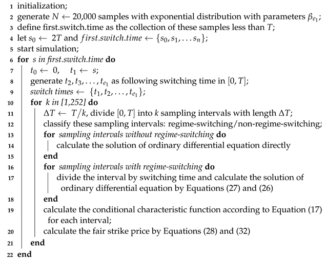
Moreover, we provide an algorithm (Algorithm 1) that calculates the fair strike price for a variance swap. Here, we only take $K_1$ as an example.

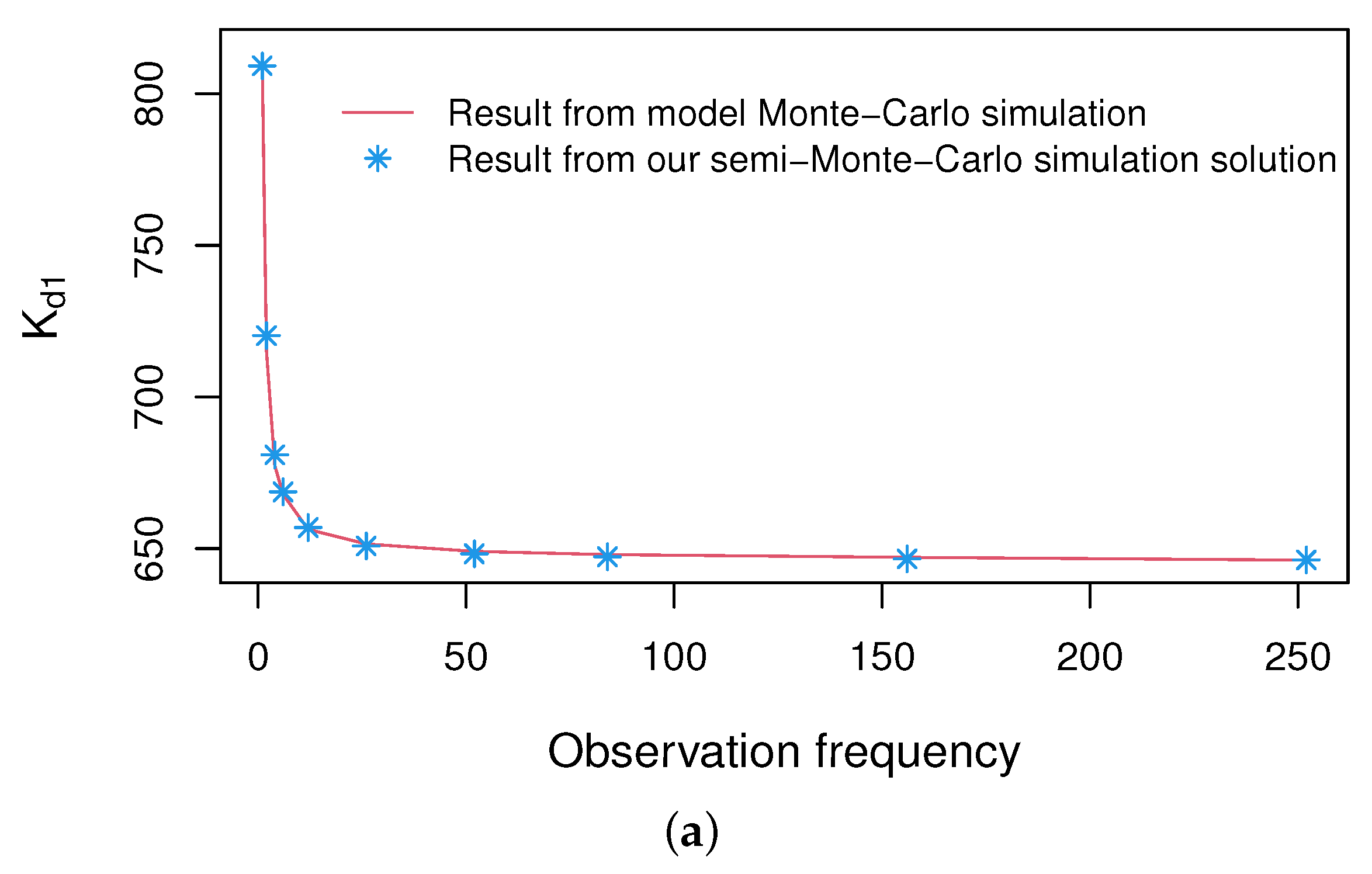
Figure 1 shows images of the fair strike price obtained from semi-Monte Carlo simulation of Equation (28) and those calculated by Monte Carlo simulation under different observation frequencies ranging from 4 to 252. Actually, the observation frequencies represent the number of trading days in a year, with 4 and 252 representing quarterly and daily observations, respectively.

Algorithm 1: Calculation of the strike price

It is evident that our solutions match the simulations well, which effectively verifies the accuracy of our pricing formulae. Furthermore, our pricing formula has higher computational efficiency, with a simulation time of 11.30401 s. In contrast, the Monte Carlo simulation time for the model requires 3.962049 min (using the simulation running time of $K_{d_1}$ as an example).

5.2. Regime-Switching Effect

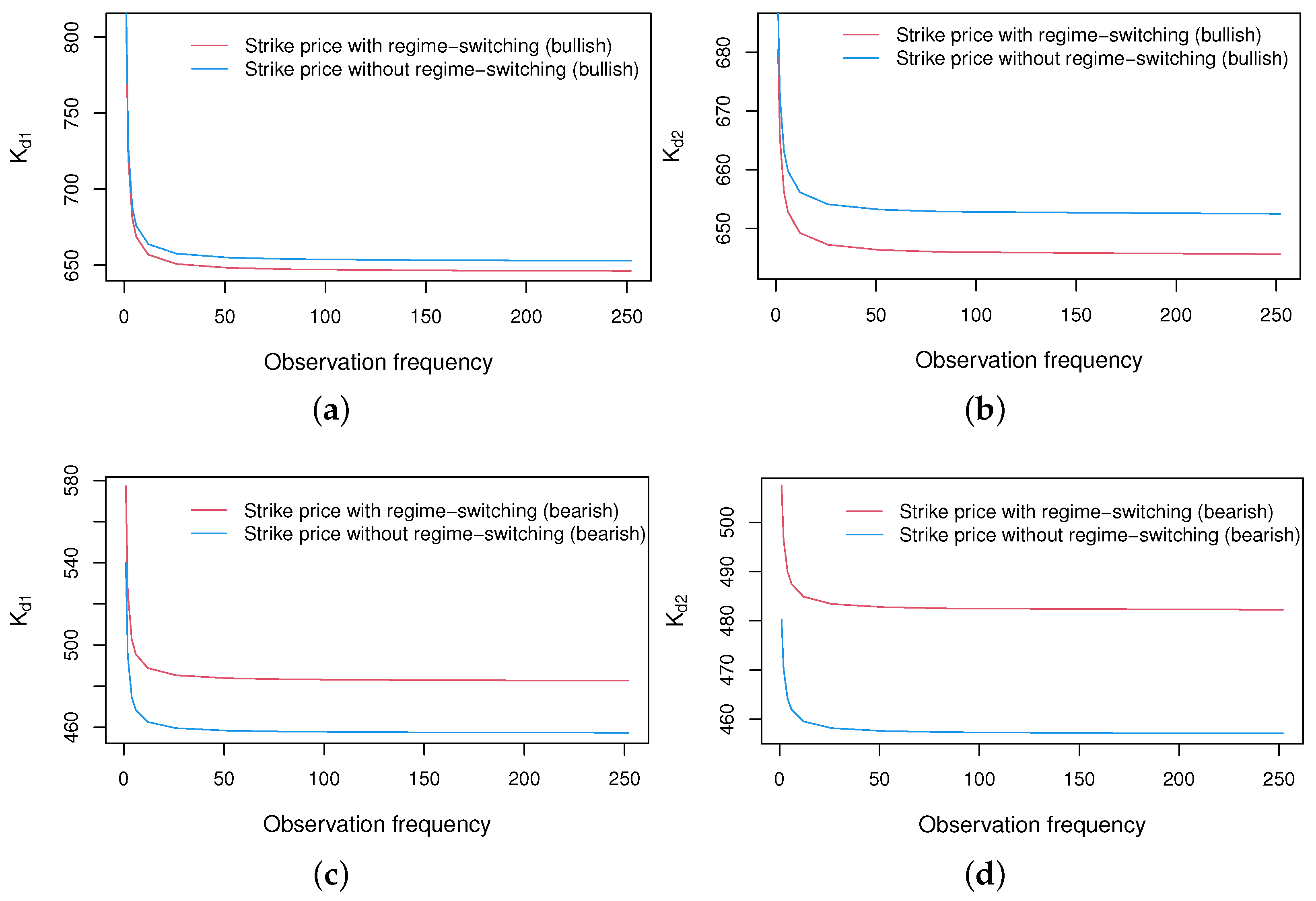
In this section, we will compare the fair strike price $K_{d_i},i=1,2$ computed from the regime-switching hybrid model and the non-regime-switching hybrid model, as shown in Figure 2. Here, the $K_{d_i},i=1,2$ without regime switching mainly refer to the situation where the model parameters are kept constant at the initial regime value throughout the entire contract period T. For example, if the initial regime is bearish, then the model parameters during the maturity T are all the values under regime 2.

Figure 2 shows that the price $K_{d_i},i=1,2$ can be significantly impacted by regime switching. More specifically, the regime tends to lower $K_{d_i},i=1,2$ to some level when it switches from a bull to a bear regime. On the other hand, when the regime switches from a bear to a bull regime, the price tends to rise somewhat. At the same time, we also observe that $K_{d_i},i=1,2$ are relatively higher when the initial regime is in a bull state (regime 1) compared to when the market regime is in a bear state (regime 2), which is consistent with the findings in [4] and real financial markets. Particularly, when the observation frequencies rises from quarterly to daily, we keep track of the price under regime 1 (see

Table 2. Fair strike price under various observation frequencies (regime 1).

Observation Frequency	${\mathit{K}}_{{\mathit{d}}_1}$ (Regime- Switching)	${\mathit{K}}_{{\mathit{d}}_2}$ (Regime- Switching)	${\mathit{K}}_{{\mathit{d}}_1}$ (Non-Regime- Switching)	${\mathit{K}}_{{\mathit{d}}_2}$ (Non-Regime- Switching)
Quarterly (N = 4)	684.6565	655.9717	685.9228	661.9446
Monthly (N = 12)	670.1038	650.0076	663.4953	657.1487
Fortnightly (N = 26)	657.2872	647.8999	657.8372	656.8177
Weekly (N = 52)	651.1446	646.8401	655.0941	654.8623
Daily (N = 252)	645.4533	645.5934	652.4541	654.7870

).

Furthermore, we can see from Table 2 that $K_{d_1}$ is considerably higher than $K_{d_2}$, and regime switching can result in large variations in $K_{d_2}$. This is mostly due to the fact that (6) prioritizes describing the relative volatility of asset prices, whereas (5) focuses more on the intensity of asset price swings.

5.3. Jump Diffusion Effect

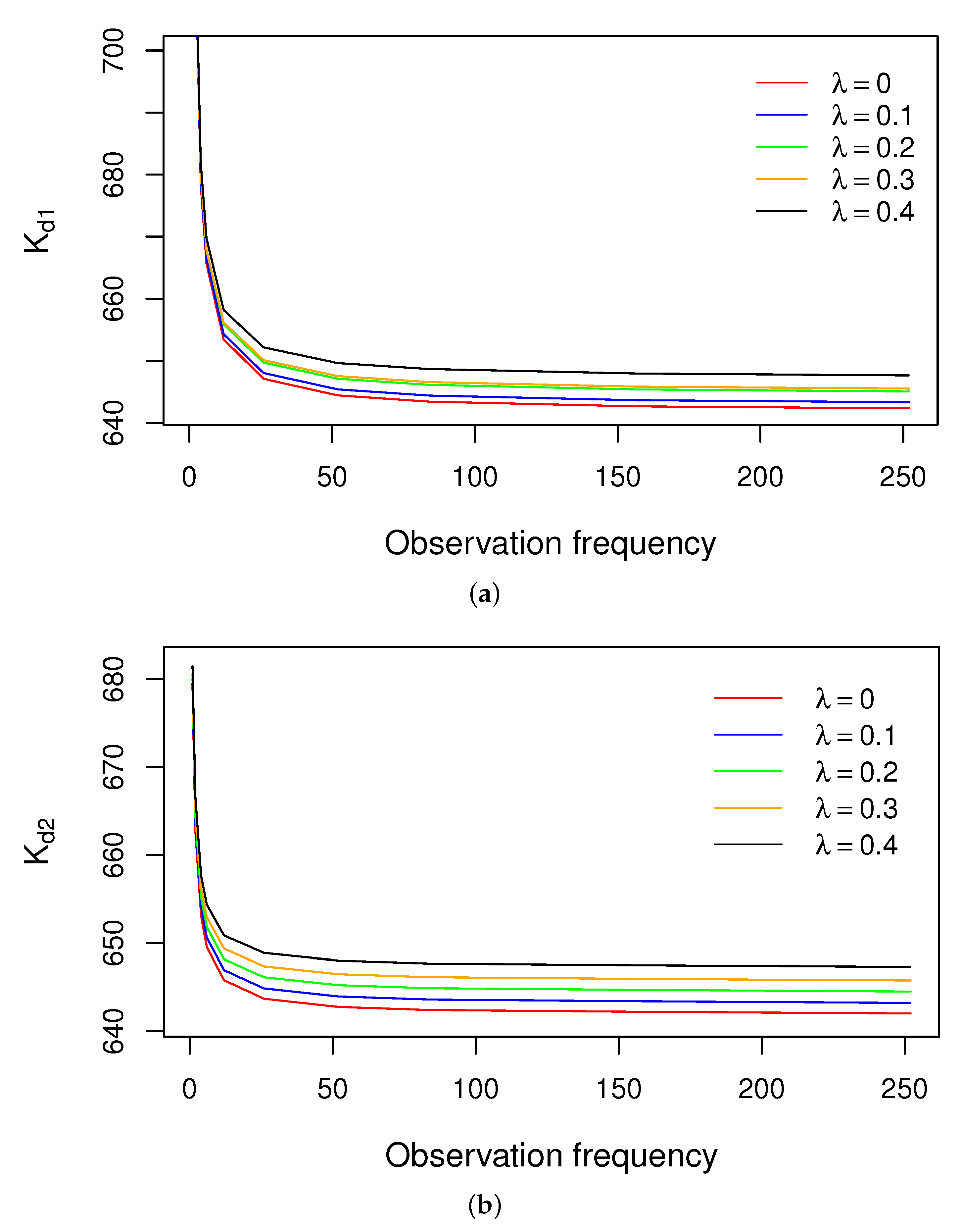
In this section, we will investigate the impact of jump diffusion by comparing the fair strike prices $K_{d_i},i=1,2$ with different jump intensities ${\tilde{\lambda }}_{{}_{X\left(t\right)}}$. Unless otherwise specified, we assume that there is no jump effect in the stock price process when ${\tilde{\lambda }}_{{}_{X\left(t\right)}}=0$. Since the major concern in this section is not the regime-switching effect, we choose to explore the jump diffusion effect under regime 1. Figure 3 shows $K_{d_i},i=1,2$ at different observation frequencies as the jump intensity ${\tilde{\lambda }}_{{}_{X\left(t\right)}}$ increases from 0 to 0.4.

From Figure 3, we can observe that at each observation frequency, the jump in $S\left(t\right)$ leads to higher prices, and as the jump intensity ${\tilde{\lambda }}_{{}_{X\left(t\right)}}$ increases, the prices further increase. One possible explanation for this is that jump diffusion may lead to changes in the underlying asset prices, resulting in higher realized variances and higher prices.

5.4. Sensitivity Analysis

In this section, we will examine the sensitivity of our model parameters by computing the fair strike prices $K_{d_i},i=1,2$ on the $1\%$ change in it. As regime switching and observation frequency are not the main concern in this section, we consider the sensitivity of parameters under daily sampling and the initial state of regime 1.

Table 3. Model parameters sensitivity analysis.

Parameters	Value	Percent Change in ${\mathit{K}}_{{\mathit{d}}_1}$	Percent Change in ${\mathit{K}}_{{\mathit{d}}_2}$
$v\left(0\right)$	0.22	0.71237780	0.71249860
$S\left(0\right)$	1.00	0.00000000	0.00000000
${\tilde{\theta }}_{{}_{X\left(t\right)}}$	$\sqrt{0.075}$	1.230927000	1.23111800
k	2.00	0.10457790	0.10459840
$\sigma$	0.10	0.05727434	0.05774045
$r_{{}_{X\left(t\right)}}$	0.08	0.001387612	0.00043574
$\rho$	−0.40	−0.00031455	0.00015732
${\tilde{\lambda }}_{{}_{X\left(t\right)}}$	0.30	0.00606860	0.00587247
p	0.20	0.00270267	0.00222682
${\eta }_1$	25.00	−0.00725323	−0.00598776
${\eta }_2$	50.00	−0.00538579	−0.00594781

shows the percentage change in $K_{d_i},i=1,2$ caused by changes in model parameters.

From Table 3, we can see that the three parameters—long-term volatility mean ${\tilde{\theta }}_{{}_{X\left(t\right)}}$, initial volatility $v\left(0\right)$, and mean reversion speed of volatility k—have a significant impact on the volatility of fair execution prices $K_{d_i},i=1,2$. Furthermore, changes in k have the most significant impact on the volatility of prices. This is consistent with the real financial market, where asset price volatility is primarily related to the stochastic volatility process of the asset price. Additionally, we find that the initial stock price $S\left(0\right)$ has no impact on the volatility of fair execution price $K_{d_i}.i=1,2$.

5.5. Comparison of the New Model with the Traditional MRG Model

In this section, we will consider the fair strike price under different models and examine how the inclusion of more realistic factors influences price. In other words, we will compare the fair strike price under the new model illustrated in (8) with prices derived from the traditional MRG model.

Both the Heston model and the MRG model are classic models in the stochastic field, and it would be comprehensive to compare our new model with both of them. However, as pointed out by Zhang [14], the connection between the MRG model and the Heston model can be made clear under a specific assumption—that the long-term average value of volatility $\tilde{\theta }$ is equal to zero. Therefore, in this section, we will focus on comparing our new model with the traditional MRG model only. Recall that the traditional MRG models assume a continuous price process with stochastic volatility, and all the parameters in the models are constant. To maintain this setting, we suppose that the parameters in the traditional models are all set in regime 1, and non-regime switching occurs in maturity.

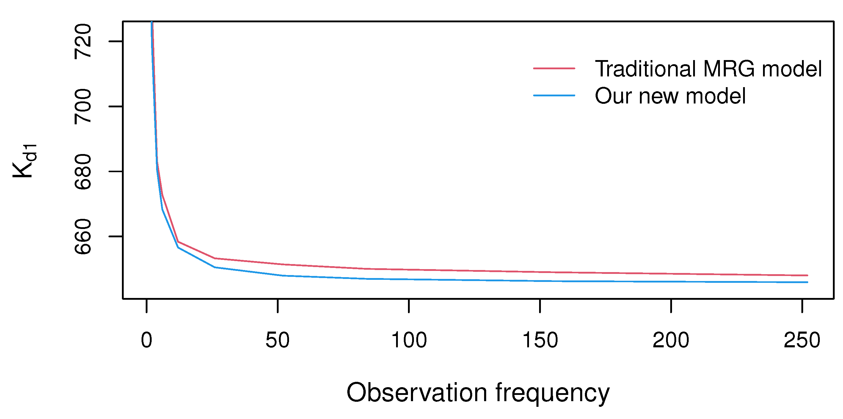
It should be noted that MRG model may not adequately capture the long-term trends in the financial market that are influenced by structural changes in macroeconomic conditions. However, empirical finance literature extensively documents the correlation between the financial market and the macroeconomic environment. Moreover, sudden and unexpected events in real-world financial markets can result in significant fluctuations in asset prices, which cannot be disregarded, especially when pricing volatility derivatives. Therefore, adding the assumption in our new model can make it more comprehensive and meaningful. Figure 4 shows the strike prices obtained from Zhang’s [14] formula and ours. (Here, we only take $K_{d_1}$ as an example to show the difference.)

From Figure 4, we can see that the price under our new model is cheaper than the one in the traditional MRG model. This can be explained as follows. First, both regime switching and jump diffusion contribute to the variation of the strike price, as discussed in the previous subsection. Second, this can be interpreted by the assumption that the parameters in the traditional MRG model are all set in regime 1 (good economy), which is larger than the ones in regime 2 (bad economy). In other words, a bearish market can drag down the price to some extent. Moreover, the small value of the long-term volatility mean may lead to a lower jump probability, meaning that the regime-switching effect has a greater effect on the price than the jump-diffusion effect. The sensitivity analysis in Table 3 can provide some evidence.

6. Conclusions

In this paper, we investigate the fair strike prices for discretely sampled variance swaps under the Markov-modulated MRG model with asymmetric double exponential jump diffusion. Compared to recent work in the variance swaps pricing field, the major contribution of this paper is to propose an effective approach to obtain a general pricing formula and improve the computational efficiency of semi-Monte Carlo simulation. The pricing problem can be reduced to an expectation calculation under the risk-neutral T-forward measure. We obtain analytical solutions for the pricing problem using the characteristic function and the conditional transition characteristic function. Additionally, we carry out a series of semi-Monte Carlo simulations to verify the accuracy and effectiveness of the pricing formulae. Our experiments aim to explore the influence of regime-switching and jump-diffusion terms, as well as analyze the sensitivity of pricing formulae parameters to the fair strike price. We find that when regime switching occurs, either the fair strike price for good economics will decrease or the fair strike price for bad economics will increase. When there is a jump in market asset prices, the diffusion of the jump will accelerate changes in stock prices, resulting in higher fair execution prices. In addition, we also find that the stochastic fluctuation parameters of the propagation model are more sensitive to price fluctuations.

Furthermore, we would like to emphasize the practical applications of our model. The pricing method proposed in our proposition is generalizable and provides a new way to accurately compute Markov-modulated variables. This approach can also be extended to other regime-switching stochastic models. For example, it could simplify the pricing formulae presented in Elliott [25] and Yang [4] without the need for overly complex expressions. Our attempt to price variance swaps under this new model can provide valuable insights and numerical evidence for financial institutions and investors to better manage and control market volatility risk, ultimately reducing trading losses.

However, it is a pity that we do not deeply consider the effect of a long contract life where the interest rate can change stochastically. In other words, if the interest rate is assumed to follow a specific stochastic process instead of a deterministic one, the ultimate risk-neutral measure and pricing formulae may differ. It would be worthwhile to explore how to adjust the pricing approach in such cases for future studies. Moreover, it would be worthwhile to explore reasonable methods for calibrating model parameter values, which we lack in this paper and hope that future research can address.

References

1. Demeterfi, K.; Derman, E.; Kamal, M.; Zou, J. More than you ever wanted to know about volatility swaps. Goldman Sachs Quant. Strateg. Res. Notes 1999, 41, 1–56. [Google Scholar]
2. Zhu, S.-P.; Lian, G.-H. Analytically pricing volatility swaps under stochastic volatility. J. Comput. Appl. Math. 2015, 288, 332–340. [Google Scholar] [CrossRef]
3. Carr, P.; Lee, R. Volatility derivatives. Annu. Rev. Financ. Econ. 2009, 1, 319–339. [Google Scholar] [CrossRef] [Green Version]
4. Yang, Y.; Liu, S.; Yonghong Wu, Y.; Wiwatanapataphee, B. Pricing of volatility derivatives in a heston–cir model with markov-modulated jump diffusion. J. Comput. Appl. Math. 2021, 393, 113–277. [Google Scholar] [CrossRef]
5. Ait-Sahalia, Y.; Karaman, M.; Mancini, L. The Term Structure of Variance Swaps and Risk Premia; Swiss Finance Institute Research Paper; Swiss Finance Institute: Zürich, Switzerland, 2018; pp. 18–37. [Google Scholar]
6. Heston, S.L.; Nandi, S. Derivatives on Volatility: Some Simple Solutions Based on Observables; Federal Reserve Bank of Atlanta WP: Atlanta, GA, USA, 2000. [Google Scholar]
7. Sepp, A. Pricing options on realized variance in the heston model with jumps in returns and volatility. J. Comput. Financ. 2008, 11, 33–70. [Google Scholar] [CrossRef] [Green Version]
8. Carr, P.; Lee, R. Hedging variance options on continuous semimartingales. Financ. Stochastics 2010, 14, 179–207. [Google Scholar] [CrossRef]
9. Swishchuk, A. Modeling of variance and volatility swaps for financial markets with stochastic volatilities. WILMOTT Mag. 2004, 2, 64–72. [Google Scholar]
10. Broadie, M.; Jain, A. Pricing and hedging volatility derivatives. J. Deriv. 2008, 15, 7–24. [Google Scholar] [CrossRef] [Green Version]
11. Zhu, S.-P.; Lian, G.-H. A closed-form exact solution for pricing variance swaps with stochastic volatility. Math. Financ. Int. J. Math. Stat. Financ. Econ. 2011, 21, 233–256. [Google Scholar]
12. Broadie, M.; Jain, A. The effect of jumps and discrete sampling on volatility and variance swaps. Int. J. Theor. Appl. Financ. 2008, 11, 761–797. [Google Scholar] [CrossRef]
13. Rujivan, S.; Zhu, S.-P. A simplified analytical approach for pricing discretely-sampled variance swaps with stochastic volatility. Appl. Math. Lett. 2012, 25, 1644–1650. [Google Scholar] [CrossRef] [Green Version]
14. Zhang, L.-W. A closed-form pricing formula for variance swaps with mean-reverting gaussian volatility. ANZIAM J. 2014, 55, 362–382. [Google Scholar]
15. Lian, G.; Chiarella, C.; Kalev, P.S. Volatility swaps and volatility options on discretely sampled realized variance. J. Econ. Dyn. Control 2014, 47, 239–262. [Google Scholar] [CrossRef]
16. Cao, J.-P.; Fang, Y.-B. An analytical approach for variance swaps with an ornstein-uhlenbeck process. ANZIAM J. 2017, 59, 83–102. [Google Scholar]
17. Mao, C.; Liu, G.; Wang, Y. A closed-form pricing formula for log-return variance swaps under stochastic volatility and stochastic interest rate. Mathematics 2021, 10, 5. [Google Scholar] [CrossRef]
18. Zhu, S.P.; Lian, G.H. Pricing forward-start variance swaps with stochastic volatility. Appl. Math. Comput. 2015, 250, 920–933. [Google Scholar] [CrossRef]
19. Maheu, J.M.; McCurdy, T.H. Identifying bull and bear markets in stock returns. J. Bus. Econ. Stat. 2000, 18, 100–112. [Google Scholar]
20. Elliott, R.J.; Lian, G.-H. Pricing variance and volatility swaps in a stochastic volatility model with regime switching: Discrete observations case. Quant. Financ. 2013, 13, 687–698. [Google Scholar] [CrossRef]
21. Bo, W.; Ruili, S. The memms for markov-modulated gbms. Chin. J. Appl. Probab. Stat. 2013, 29, 179–187. [Google Scholar]
22. Elliott, R.J.; Chan, L.; Siu, T.K. Option pricing and esscher transform under regime switching. Ann. Financ. 2005, 1, 423. [Google Scholar] [CrossRef]
23. Liao, J.; Shu, H.; Wei, C. Pricing power options with a generalized jump diffusion. Commun.-Stat.-Theory Methods 2017, 46, 11026–11046. [Google Scholar] [CrossRef]
24. Bo, L.; Wang, Y.; Yang, X. Markov-modulated jump–diffusions for currency option pricing. Insur. Math. Econ. 2010, 46, 461–469. [Google Scholar] [CrossRef]
25. Elliott, R.J.; Siu, T.K.; Chan, L. Pricing volatility swaps under heston’s stochastic volatility model with regime switching. Appl. Math. Financ. 2007, 14, 41–62. [Google Scholar] [CrossRef]
26. Lin, S.; He, X.-J. Analytically pricing variance and volatility swaps with stochastic volatility, stochastic equilibrium level and regime switching. Expert Syst. Appl. 2023, 217, 119592. [Google Scholar] [CrossRef]
27. Hamilton, J.D. Regime switching models. In Macroeconometrics and Time Series Analysis; Palgrave Macmillan: London, UK, 2010; pp. 202–209. [Google Scholar]
28. Gatheral, J. The Volatility Surface: A Practitioner’s Guide; John Wiley & Sons: New York, NY, USA, 2011. [Google Scholar]
29. Tankov, P. Financial Modelling with Jump Processes; Chapman and Hall/CRC: Boca Raton, FL, USA, 2003. [Google Scholar]
30. Kou, S.G. A jump-diffusion model for option pricing. Manag. Sci. 2002, 48, 1086–1101. [Google Scholar] [CrossRef] [Green Version]
31. Huang, J.; Zhu, W.; Ruan, X. Option pricing using the fast fourier transform under the double exponential jump model with stochastic volatility and stochastic intensity. J. Comput. Appl. Math. 2014, 263, 152–159. [Google Scholar] [CrossRef]
32. Vo, M.T. Regime-switching stochastic volatility: Evidence from the crude oil market. Energy Econ. 2009, 31, 779–788. [Google Scholar] [CrossRef]
33. Yang, H. Esscher transform. Wiley Statsref Stat. Ref. Online 2014. [Google Scholar] [CrossRef]
34. Merton, R.C. Option pricing when underlying stock returns are discontinuous. J. Financ. Econ. 1976, 3, 125–144. [Google Scholar] [CrossRef] [Green Version]
35. Shreve, S.E. Stochastic Calculus for Finance II: Continuous-Time Models; Springer: Berlin/Heidelberg, Germany, 2004; Volume 11. [Google Scholar]
36. Buffington, J.; Elliott, R.J. American options with regime switching. Financ. Stochastics 2002, 5, 497–514. [Google Scholar] [CrossRef]
37. Buffington, J.; Elliott, R.J. Regime switching and european options. In Stochastic Theory and Control: Proceedings of a Workshop Held in Lawrence, Kansas; Springer: Berlin/Heidelberg, Germany, 2002; pp. 73–82. [Google Scholar]
38. Liu, S.; Yang, Y.; Zhang, H.; Wu, Y. Variance swap pricing under markov-modulated jump-diffusion model. Discret. Dyn. Nat. Soc. 2021, 2021, 9814605. [Google Scholar] [CrossRef]
Figure 1. Comparison of the fair strike price obtained from model Monte Carlo simulation and our semi-Monte Carlo simulation. (a) K d 1 with regime 1. (b) K d 2 with regime 1.
Mathematics 11 02730 g001aMathematics 11 02730 g001b
Figure 2. Comparison of the fair strike price obtained from regime-switching or non-regime-switching models. (a,b) K d i , i = 1 , 2 with regime 1. (c,d) K d i , i = 1 , 2 with regime 2.
Mathematics 11 02730 g002
Figure 3. Comparison of the fair strike price obtained from various jump intensities. (a) K d 1 with regime 1. (b) K d 2 with regime 1.
Mathematics 11 02730 g003
Figure 4. Comparison of the fair strike price obtained under the traditional MRG model with our new model.
Mathematics 11 02730 g004