Article

Enhancing Precision in Large-Scale Data Analysis: An Innovative Robust Imputation Algorithm for Managing Outliers and Missing Values

School of Business, University of Applied Sciences and Arts Northwestern Switzerland, 4600 Olten, Switzerland
Mathematics 2023, 11(12), 2729; https://doi.org/10.3390/math11122729
Submission received: 31 May 2023 / Revised: 13 June 2023 / Accepted: 14 June 2023 / Published: 16 June 2023

Abstract

:
Navigating the intricate world of data analytics, one method has emerged as a key tool in confronting missing data: multiple imputation. Its strength is further fortified by its powerful variant, robust imputation, which enhances the precision and reliability of its results. In the challenging landscape of data analysis, non-robust methods can be swayed by a few extreme outliers, leading to skewed imputations and biased estimates. This can apply to both representative outliers—those true yet unusual values of your population—and non-representative outliers, which are mere measurement errors. Detecting these outliers in large or high-dimensional data sets often becomes as complex as unraveling a Gordian knot. The solution? Turn to robust imputation methods. Robust (imputation) methods effectively manage outliers and exhibit remarkable resistance to their influence, providing a more reliable approach to dealing with missing data. Moreover, these robust methods offer flexibility, accommodating even if the imputation model used is not a perfect fit. They are akin to a well-designed buffer system, absorbing slight deviations without compromising overall stability. In the latest advancement of statistical methodology, a new robust imputation algorithm has been introduced. This innovative solution addresses three significant challenges with robustness. It utilizes robust bootstrapping to manage model uncertainty during the imputation of a random sample; it incorporates robust fitting to reinforce accuracy; and it takes into account imputation uncertainty in a resilient manner. Furthermore, any complex regression or classification model for any variable with missing data can be run through the algorithm. With this new algorithm, we move one step closer to optimizing the accuracy and reliability of handling missing data. Using a realistic data set and a simulation study including a sensitivity analysis, the new alogorithm imputeRobust shows excellent performance compared with other common methods. Effectiveness was demonstrated by measures of precision for the prediction error, the coverage rates, and the mean square errors of the estimators, as well as by visual comparisons.

1. Introduction

The CRISP data mining model [1] is a widely used framework for data mining projects. The name CRISP stands for Cross-Industry Standard Process for Data Mining, and the model consists of six major phases, with data cleaning as one of the essential phases. This is also true for similar data mining models, e.g., the GSBPM (Generic Statistical Business Process Model) [2], which is a data process model used by national statistical offices and other organizations for organizing their statistical work, and its fourth out of seven main steps reports about data cleaning and the imputation of missing values. This underlines the importance of data cleaning and the imputation of missing values as one intergrative part of data processing and analysis.
Furthermore, current literature on data cleaning reports that missing values are crucial to address [3], shows the imputation of missing values as one integrative part [4], and addresses the problems of missing values, see e.g., [5], and some of them are already discussing robust imputation methods [6,7].
The imputation of missing values is undoubtedly an essential part of data science applications.

1.1. Different Types of Missing Data: MCAR, MAR, and MNAR

Data are said to be MCAR if the probability of missingness is the same for all units. In other words, the event of missingness, denoted as R (where R = 1 for observed and R = 0 for missing), is independent of both observed ( Y o b s ) and unobserved ( Y m i s ) data. The parameters ϕ refer to unknowns in the distribution of the data or the process that led to the missingness. The inclusion of these parameters underscores that whether the data is MCAR, MAR, or MNAR cannot usually be determined definitively from the data alone and instead involves untestable assumptions about these unknowns.
P ( R = 1 | Y o b s , Y m i s , ϕ ) = P ( R = 1 , ϕ )
For example, if we’re collecting data on people’s height and weight and some heights are missing simply because the machine measuring height malfunctioned randomly, then that missing data would be MCAR.
The situation is missing at random (MAR) if the probability of missingness depends on the observed data but not on the unobserved data:
P ( R = 1 | Y o b s , Y m i s , ϕ ) = P ( R = 1 | Y o b s , ϕ )
For example, suppose men are less likely than women to answer a question about weight. Furthermore, given that we know a person’s gender, their propensity to skip the weight question is unrelated to their actual weight.
Missing Not at Random (MNAR) is the case if the probability of missingness depends on the unobserved data:
P ( R = 1 | Y o b s , Y m i s , ϕ ) P ( R = 1 | Y o b s , ϕ )
For instance, if people with higher weights are more likely to skip a weight question, then the missingness of weight data is directly related to the unobserved missing weight data. This includes cases where missingness depends on both observed and unobserved data, or just the unobserved data.
In this contribution, we focus only on the MAR case. MAR is a widely used and crucial assumption for many statistical procedures dealing with missing data.

1.2. Imputation Uncertainty, Multiple Imputation, and Model Uncertainty

When we handle missing data through imputation, we are dealing with inherent uncertainties. These well-known uncertainties [7,8] can generally be classified into two main categories: imputation uncertainty and model uncertainty. Additionally, multiple imputation estimates several values for each missing value, thus considering that an imputed value is not a fixed value but derives from a distribution.

1.2.1. Imputation Uncertainty

This pertains to the uncertainty in the imputed values themselves. When we impute missing data, we’re essentially making an educated guess about what the missing values could have been, given the observed data and the assumptions we’ve made. This guess is inherently uncertain because the real values could actually have been different. To incorporate this uncertainty into our imputation, we typically don’t just fill in the missing value with a single best guess (like the predicted mean). Instead, we add some noise to our guess or draw from the predictive distribution. This reflects our uncertainty about the exact value of the missing data. For example, suppose we’re dealing with missing values in a continuous variable and we’re using a linear regression model to predict the missing values. Instead of just filling in the missing value with the predicted mean from the regression model, we could add a random residual to this mean (where the residual is drawn from the distribution of residuals in the observed data). This is known as stochastic regression imputation, and it is one way to incorporate imputation uncertainty.

1.2.2. Multiple Imputation

With the above considerations, we impute—albeit with noise to account for natural variability—with fixed values, but in reality we cannot assume a fixed value, but a distribution for a missing value. This problem is absorbed by multiple imputations. Multiple imputation involves creating multiple datasets where the missing values are replaced with plausible values based on the distribution of the observed data. Each of these “completed” datasets is then analyzed, and the results are pooled to create an overall result that takes into account the uncertainty about what the missing data could be.

1.2.3. Model Uncertainty

Model uncertainty plays only a role for random samples but not for census data. This pertains to the uncertainty in the model used for imputation. When we use a model (like a linear regression model) to predict missing values, we’re making assumptions about the underlying data-generating process. These assumptions are inherently uncertain because the true data-generating process could actually be different. To incorporate this uncertainty into our imputation, we typically use methods such as bootstrap or Bayesian regression that recognize our model as just one possible model out of many. These methods essentially allow for a range of possible models, each with its own set of predictions for the missing values. For example, suppose again that we’re using a linear regression model to predict missing values. We could bootstrap our data (i.e., repeatedly draw random samples from our data with replacement) and fit a separate regression model to each bootstrap sample. This would give us a range of regression models, each with slightly different coefficients. We could then use each model to generate a separate imputed dataset, resulting in multiple imputed datasets that reflect our model uncertainty.
By incorporating both imputation uncertainty and model uncertainty into our missing data handling, we can make more accurate inferences that honestly reflect the inherent uncertainties involved. It is worth noting that imputation methods used in the context of multiple imputation must include randomness for model uncertainties (e.g., using a bootstrap or Bayesian methods) and for imputation uncertainties where a random number generator is used to select one of the plausible values to replace the missing data point.

1.3. The Problem with Outliers

Outliers in a dataset can significantly influence statistical analyses, and therefore, it’s crucial to understand the different types. Outliers are generally divided into two categories: representative and non-representative [9].

1.3.1. Representative Outliers

These are data points that are far from the rest of the data but are genuine observations. They provide valid information about the variability in the data and are not the result of an error or anomaly in data collection. For example, in a data set on household income, the incomes of billionaires would be representative outliers. These are true, albeit rare, observations that genuinely exist in the population. Removing these outliers from the dataset could lead to biased results because it would artificially reduce the observed variability in the data. However, they can influence non-robust imputation methods dramatically. For example, with regression imputation, they might (completely) leverage out the regression fit so that the fit does not describe the data well. Using such a fit to impute missing values would result in unrealistic imputed values just because the regression was leveraged by outliers. Leaving them out so that the non-robust fit of a non-robust imputation method is not leveraged is not a good idea since the sample size is reduced and it is also challenging to detect the outliers.

1.3.2. Non-Representative Outliers

These are data points that are also far removed from the rest of the data, but they do not provide valid information about the general trend or variability of the data. They are usually the result of errors, such as measurement errors, data entry errors, or experimental anomalies. For instance, if a person’s height is recorded as 250 cm due to a typo instead of the correct 150 cm, this value would be a non-representative outlier. Non-representative outliers should be corrected when applying non-robust imputation methods, if possible, as they can distort the true pattern in the data and lead to misleading conclusions. However, unlike for representative outliers, it is a challenge to detect non-representative outliers and replace them [10]. It is more convenient to use robust imputation methods at first glance.
In addition, distinguishing between representative and non-representative outliers can be challenging, and outlier detection methods hardly distinguish between them [11]. In addition, removing outliers after outlier detection is not a good idea since it reduces the sample size and thus affects the estimation of the variance of an estimators.
By using robust imputation methods, no challenging outlier detection must be made first, and there is no need to distinguish between representative and non-representative outliers since both influence and leverage non-robust methods, and both types of outliers must thus be downweighted to reduce their influence. Without this down-weighting, fits may be completely driven by the outliers, and unrealistic imputed values may result.

1.4. Open Points and Outline

Common imputation methods, such as regression imputation, can be sensitive to outliers, meaning that the presence of outliers can dramatically influence the imputed values. In addition, common frameworks such as MICE do not allow for complex models (e.g., with interaction terms between predictors or the use of polynomials) for each variable to impute, and model misspecifications are common even without outlying observations.
A way out to the latter point is to use random forests or XGBoost to impute missing values. However, even imputation with random forests or XGBoost can be strongly influenced by outliers in the response variable. Imputation methods such as imputation with MICE using PMM (see Algorithm A3 and [12]), as well as outliers in the predictor space in particular, can lead to model misspecification, and local outliers in the response variable near the imputed value can strongly influence the imputations.
IRMI [6], described in Section 2.1, performs robust imputation but does not account for model uncertainty. Drawing a bootstrap sample and then fitting IRMI would be trivial, but outliers might be overrepresented in a bootstrap sample and undermine the robustness properties of robust methods. In Section 2.3, we therefore formulate a robust bootstrap based on the ideas of ref. [13].
Even with IRMI, complex models cannot be passed through the algorithm. The new algorithm imputeRobust, explained in Section 2.4, allows for this and also uses a robust bootstrap to account for outliers and model uncertainty.
Section 2.5 explains the evaluation criteria used to assess the effectiveness of imputeRobust and the compared methods. The results in Section 3.1 show why the integration of complex models is so important, and Section 3.2 shows the results of a simulation and a sensitivity analysis. Furthermore, the carbon footprint of our algorithm is roughly outlined in Section 3. Section 4 discusses the results in a broader context, draws conclusions, and summarizes all findings.

2. Materials and Methods

2.1. Robust Imputation

The iterative robust model-based imputation (IRMI) algorithm (see a rough summary in Algorithm 1), proposed by ref. [6], is an effective procedure for handling missing data. It is especially suited for dealing with multivariate datasets where observations may be missing at random. The key steps of the IRMI algorithm can be summarized as follows:
Algorithm 1 Iterative Stepwise Robust Model-Based Imputation (IRMI).
1:
Initialize: Impute missing values using kNN imputation.
2:
repeat
3:
    for each variable j with missing values do:
4:
       (a) Regress j using a robust method (choice depends on the scale of the variable to impute) on all other variables using observations where j is not missing.
5:
       (b) Predict the missing values in j using the estimates from the model.
6:
    update: Replace the missing values in variable j with the noised predictions. This noise is adequately chosen to consider imputation uncertainty.
7:
    end for
8:
until convergence (changes in the imputed values fall below a specified threshold)
There are many details about this algorithm that are not mentioned here. We refer to [6].
The IRMI algorithm is robust to outliers and can handle different types of variables (continuous, categorical, count, etc.). It iterates between model estimation and imputation until the changes in the imputed values are smaller than a specified threshold, indicating convergence. The algorithmic complexity depends on the number of missing values and the chosen regression method. IRMI allows for multiple imputations and imputation uncertainty but does not consider model uncertainty. In addition, only simple models per variable can be passed through (so as for MICE).

2.2. Problems in Taking Model Uncertainty into Account with Robust Imputation

One way of considering model uncertainty is to draw bootstrap samples (with replacement) from the data and fit the model to the bootstrap samples. Another approach is to draw residuals and add them to the fitted values of the response before re-fitting the model (residual bootstrap). In this contribution, we do not consider the residual bootstrap.
However, the bootstrap method can be problematic when the data contain outliers, even when robust statistical methods are used for fitting a model.
When you have a fair amount of outliers in your data, outliers can get overrepresented, i.e., it can happen that more than 50% of your bootstrapped data set are then outliers. More precisely, since bootstrap involves resampling with replacement, outliers can get selected multiple times in the resampled data. This can lead to an overrepresentation of the outliers, and therefore, the bootstrap distribution may be heavily influenced by these outliers.

2.3. Robust Bootstrap

The Robust Bootstrap method proposed by ref. [13] is a variation of the traditional bootstrap that aims to decrease the influence of outliers on the bootstrap distribution. It does this by first obtaining a robust estimate of the parameter of interest and then generating bootstrap samples in a way that down-weights or excludes outliers.
In Algorithm 2, this approach is adapted to consider model uncertainty for continuous responses, and in Algorithm 3, for non-continuous variables.
This method helps to ensure that the bootstrap distribution is more representative of the underlying distribution of the data without being overly influenced by outliers or high-leverage points.
Algorithm 2 Robust Bootstrap for continuous response.
1:
procedure RobustBootstrap( D a t a , N u m B o o t s t r a p S a m p l e s )
2:
    Compute the LTS or MM regression estimator on D a t a , obtaining parameter estimates β L T S or β M M
3:
    for  i = 1 to N u m B o o t s t r a p S a m p l e s  do
4:
        Generate a bootstrap sample from D a t a with weights (probabilities to be sampled) based on residuals from the LTS or MM regression model. Outliers, defined by large residuals, should have smaller weights (MM-regression by using the robustness weights ϕ ( r i / S ) / ( r i / S ) with r i the residuals, S the robust scale estimate of residuals and ϕ the Tukey’s biweight function [14]) or be excluded (LTS-regression based on the size of the subset h, the percentage of squared residuals whose sum will be minimized).
5:
        Compute the LTS or MM regression estimator on the bootstrap sample, obtaining bootstrap parameter estimates β L T S , i or β M M , i
6:
    end for
7:
end procedure
Algorithm 3 Robust Bootstrap for categorical response.
1:
procedure RobustBootstrap( D a t a , N u m B o o t s t r a p S a m p l e s )
2:
    Estimate robust Mahalanobis distances [15]
3:
    Create a weight vector with 1’s and 0’s depending if the robust Mahalanobis distances are smaller or greater equal than χ ( p ) 2 with p the number of variables. Thus, outliers receives a weight of 0.
4:
    for  i = 1 to N u m B o o t s t r a p S a m p l e s  do
5:
        Generate a bootstrap sample from D a t a with weights (probabilities to be sampled) based on the previous step.
6:
        Apply the imputation method on the bootstrap sample, obtaining bootstrap parameter estimates.
7:
    end for
8:
end procedure

2.4. Putting It All Together: The imputeRobust Algorithm

imputeRobust is an implementation for the multiple imputation of missing data. The code aims to estimate the missing values in a dataset using robust techniques.
The input parameters to the imputeRobust algorithm are
formulas: 
a list of models. For each variable in the data a complex model formula can be provided. If no formula is provided it uses the simplest model, explaining the response with all predictor variables in the data set. Any complex model is allowed to be passed through for each variable in the data set, e.g., considering transformations of variables, quadratic terms or interactions, etc.
data: 
the dataset with missing values to be imputed.
boot, robustboot
logical flags to use bootstrapping and robust bootstrapping respectively. So if true, model uncertainty is either considered by a bootstrap or a robust bootstrap. General suggestion is to use roubstboot for random samples and no bootstrap at all for census data.
method: 
the regression method to use for imputation of continuous variables. Implemented methods are LTS regression, ordinary least squares estimation, generalised additive models using thin plate splines, MM regression.
multinom.method: 
the method to use for multinomial logistic regression, used when imputing nominal variables. Here multinomial log-linear models via neural networks are used [16].
eps: 
a numeric value specifying the stopping criterion for the iterative algorithm.
maxit: 
the maximum number of iterations for the algorithm.
alpha: 
a numeric value used for quantile calculation when using the LTS estimator.
uncert: 
a string specifying the method to generate uncertainty in the imputed values. Possible methods are to use normal errors, residual errors, midastouch or the PMM method, see Algorithm 8 for details.
Thus, imputeRobust extends MICE by enabling model formulas for each variable and by having the ability to deal with outliers, and imputeRobust extends MICE and IRMI by considering model uncertainty using a robust bootstrap.
The main steps of the algorithm are explained in Algorithms 4–8.
Algorithm 4 imputeRobust.
1:
procedure  imputeRobust(formulas, data, boot, robustboot, method, multinom.method, takeAll, eps, maxit, alpha, uncert, familiy, value_back, trace)
2:
    Initialize parameters, detect and convert character variables to factors.
3:
    Determine factor type (dichotomous or polytomous), detect problematic factors.
4:
    if takeAll is true then
5:
        Initialize the missing values using kNN imputation explained in Algorithm A2.
6:
    end if
7:
    Compute the outlier index if there are any categorical variables with missing values.
8:
    while criteria > eps and iterations < maxit do
9:
        For each variable j with missing values do:
10:
      if if boot or robustboot is true then
11:
           draw a (robust) bootstrap sample considering Algorithms 2 or 3, depending on if the response is continuous or categorical. Note that Algorithm 3 is applied outside the loop, since it must be calculated only once while Algorithm 2 must be called in the inner loop. Fit the following model on the boostrap sample.
12:
        end if
13:
         (a) Regress or classify j using a robust method (choice depends on the scale of the variable to impute) on all other variables using observations where j is not missing, see Algorithm 5 for the choice of methods and subsequent Algorithms 6 and 7.
14:
          (b) Predict the missing values in j using the estimates from the model.
15:
        Update: Replace the missing values in variable j with the noised predictions. This noise is adequately chosen to consider imputation uncertainty, see Algorithm 8.
16:
        Update value of criteria until convergence (changes in the imputed values fall below a specified threshold)
17:
    end while
18:
    return imputed data.
19:
end procedure
Algorithm 5 Imputation method selection.
1:
procedure imp(form, data, type, method, multinom.method, index, factors, boot, robustboot, uncert, outIndex)
2:
    Select method based on variable type, see Algorithm 6 and 7
3:
    return imputed values of the response, consider imputation uncertainty (Algorithm 8).
4:
end procedure
Algorithm 6 Robust imputation for nominal type.
1:
procedure useRobustMN(form, data, index, factors, boot, robustboot, uncert, multinom.method, outIndex)
2:
    Perform robust multinomial regression for imputation based on multinom.method.
3:
    return imputed values.
4:
end procedure
Algorithm 7 Robust imputation for numeric type.
1:
procedure useRobustNumeric(form, data, method, index, factors, boot, robustboot, uncert)
2:
    Perform robust regression for imputation based on method, apply bootstrapping if needed.
3:
    Generate imputed values based on specified uncertainty method (Algorithm 8).
4:
    return imputed values.
5:
end procedure
Algorithm 8 Imputation uncertainty.
1:
procedure imputationUncertainty(uncert)
2:
    if response is continuous then
3:
        if uncertainty equals normal error then
4:
           It generates normally distributed random numbers with mean 0 and (robust) standard deviation. It then adds these random numbers to the predicted values, i.e., normally distributed errors are added to the predicted values.
5:
        end if
6:
        if uncertainty equals residual error then
7:
           Samples residuals from the fitted model and adds them to the predicted values. For robust imputation, only the residuals from the non-outliers are chosen. This assumes that the variability of the missing values can be captured by the residuals of the model.
8:
        end if
9:
        if uncertainty equals weighted residual error—midastouch then
10:
           Weights residuals based on the distance to the missing point and samples a residual to add to the prediction. This is a more complex method that weights residuals based on their “closeness” in the predictor space to the point being imputed. Samples are taken using these weights as selection probabilities.
11:
        end if
12:
        if uncertainty equals PMM then
13:
           This is the well-known PMM method. For each missing value, the observed values with the closest predicted values are found and one randomly selects one of their observed values as the imputed value.
14:
        end if
15:
    end if
16:
    if response is nominal then
17:
        Draw a sample from the categories with selection probabilities based on the model fit.
18:
    end if
19:
    return imputed values.
20:
end procedure

2.5. Evaluation Criteria

The Mean Absolute Percentage Error (MAPE) is frequently used to compare the performance of different imputation methods. In this context, the MAPE is computed as the average of the absolute differences between the true values and the imputed values, divided by the absolute true values. The result is then multiplied by 100 to convert it to a percentage. Lower MAPE values indicate a better fit of the imputation method.
Given a variable y = ( y 1 , y 2 , , y n ) with true values and y ^ = ( y ^ 1 , y ^ 2 , , y ^ n ) as the corresponding imputed values, the MAPE for one variable with missings is calculated as
M A P E = 100 × 1 n ( m i s s ) i = 1 n y i y ^ i y i ,
where n ( m i s s ) is the total number of missing values. The MAPE is calculated for all variables with missing values in a data set and summed up.
The Normalized Root Mean Squared Error (NRMSE) is a standardized measure of the differences between the actual values and the predicted values from a model, namely the imputed values in this case. It is particularly useful when you want to compare the predictive performance of different models or different datasets. The NRMSE for one variable with missingness can be calculated with
N R M S E = 1 n ( m i s s ) i = 1 n ( m i s s ) y i y ^ i s 2 ,
where s is the standard deviation of the true values. Again, if there is more than one variable missing, the NRMSE is calculated for each variable and summed up.
The Mean Squared Error of Correlation (MSECor) measures the average squared difference between the correlations in two different datasets or two different versions of a dataset. It is commonly used to evaluate how well an imputation method is able to preserve the correlation structure of the original data. It can be calculated with
M S E C o r = 1 p i = 1 p j = 1 p ( c o r ( X i , X j ) c o r ( Y i , Y j ) ) 2 ,
where p is the number of variables in the dataset, c o r ( X i , X j ) is the correlation coefficient between the i-th and j-th variables in dataset X, c o r ( Y i , Y j ) is the correlation coefficient between the i-th and j-th variables in dataset Y (the imputed data set).
The coverage rate of an estimator is calculated by checking if the (only in a simulation known) true value lies within a (1 − α )% confidence interval around the estimated parameter by repeatedly simulating data, imputing data and calculating the estimator. It is given by
C R = 1 R i = 1 R I ( l i θ u i ) ,
with R the number of simulations, I is an indicator function that is equal to 1 if the condition l i < θ < u i is true and 0 otherwise, and l i and u i represent the lower and upper bounds of the confidence interval for the estimate θ . It is defined by also considering non-representative outliers. Thus, after imputation, the coverage rate and respective confidence intervals are calculated on the basis of the non-outlying observations.
The root mean squared error (RMSE) of an estimator, when estimated in a simulation, is a widely used measure of the differences between values predicted by a model or an estimator and the values observed. In the context of a simulation, we might run the simulation many times with different random inputs and compare the estimator’s output each time to the true value. For each simulation run, you calculate the (squared) error, which is the difference between the estimated value and the true value. You then calculate the mean of these squared errors across all simulation runs. The square root gives the RMSE. So, if θ ^ represents the estimator and θ represents the true value, the RMSE for n simulation runs can be written as
R M S E = 1 n i = 1 n ( θ ^ i θ ) 2
This formula provides a measure of the accuracy of the estimator. It tells you, on average, how much the estimator’s predictions deviate from the true values. The smaller RMSE signifies a better fit of the model to the data.

3. Results

3.1. Highlighting the Benefits When Allowing Complex Model Formulas

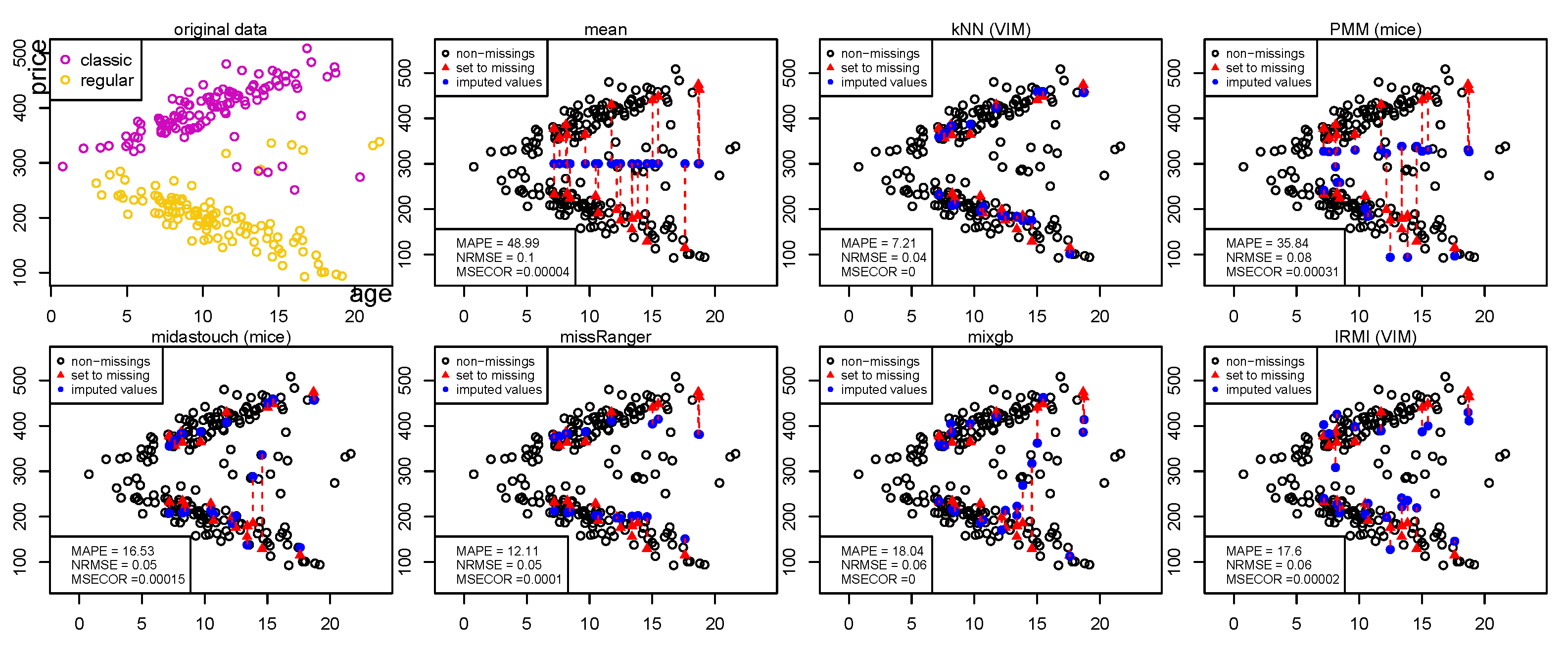
With the artificial but not unrealistic data set of Swiss watches with n = 200 observations, we want to highlight that imputeRobust can deal with any complex model formulation of a linear model. In Figure 1, top left, one can see the prices of Swiss watches depending on the age. This is the fully observed data set. Classic watches generally increase in price, while regular watches decrease in price of time. However, this is not generally true, and thus one can see some outliers in between the majority of classic and regular Swiss watches.
One question is how different imputation methods deal with such a rather simple data set when the price depends on age with interaction to the type of watch (classic or regular). We set some 10% of the prices to zero using MAR corresponding to the age of watches, indicated by red triangles in the plots in Figure 1. Various imputation methods are used to impute these introduced missing values (blue circles; see also the connecting lines to the true values), and the MAPE, NRMSE, and MSECor are reported. The (benchmarking) methods used are given in Table 1 and further explained in Appendix A. For all multiple imputation methods, only one imputed data set is shown.
Finding 1: kNN performs by far the best among the benchmarking methods. Outliers have no influence on the imputation, and accuracy is best.
Finding 2: All other methods are strongly influenced by outliers or the wrong model choice. With the exception of kNN, these are all very poor results.
Finding 3: We can very easily see that many methods are very much influenced by model misspecification, contrary to what is claimed, e.g., for PMM [8].
Figure 1 shows two different methods under three different settings for model uncertainty and four different imputation uncertainty treatments. These settings are summarized in Table 2.
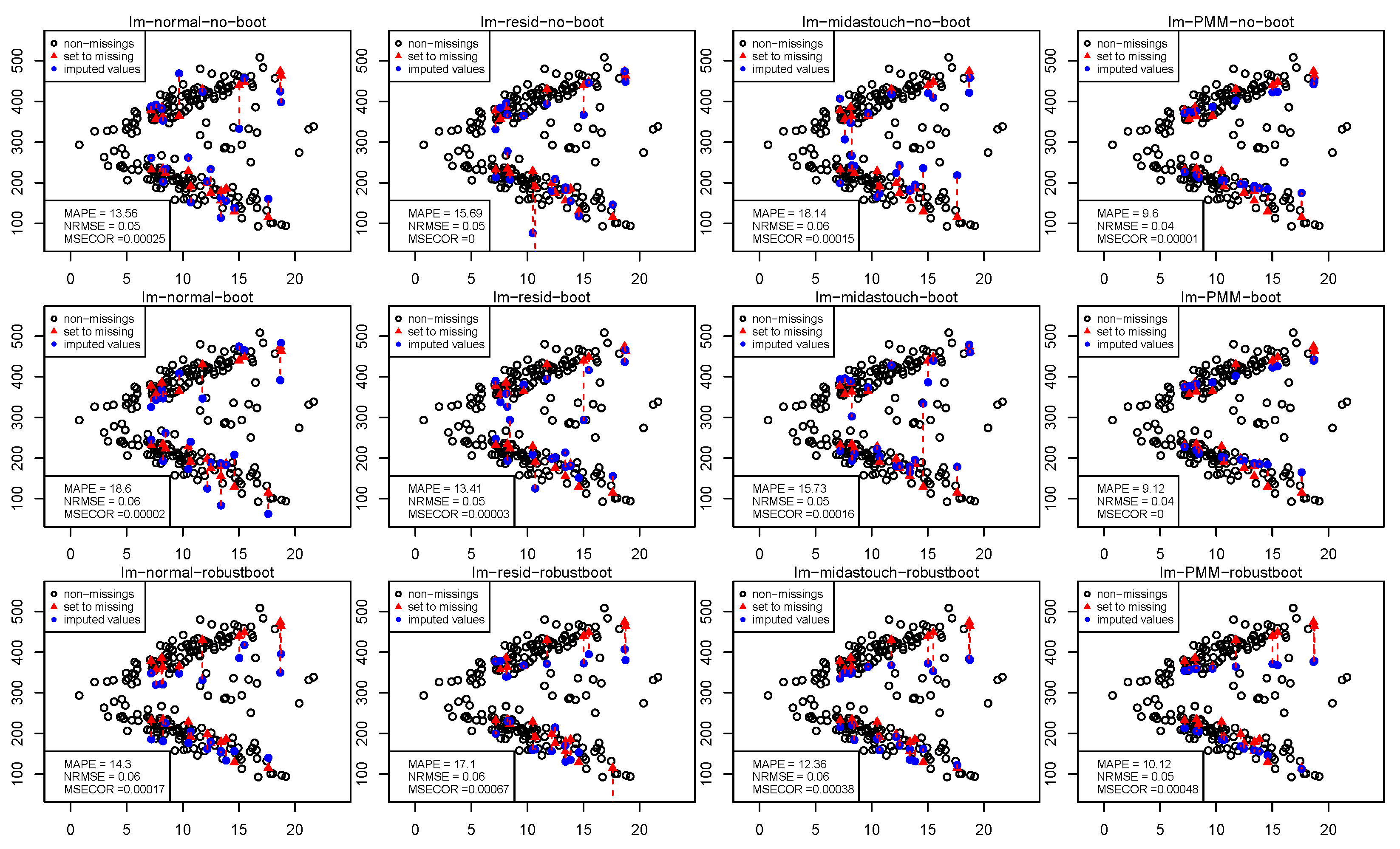
Figure 2 shows the results of the OLS regression. These results are also shown only for benchmarking purposes. Even if we have chosen the right model with the interaction terms of age of a watch and type of watch, outliers influence the results. The results improve slightly when the robust bootstrap is used.
Finding 4: A robust bootstrap improves the treatment of outliers, but a robust bootstrap is not sufficient to reduce the influence of outliers.
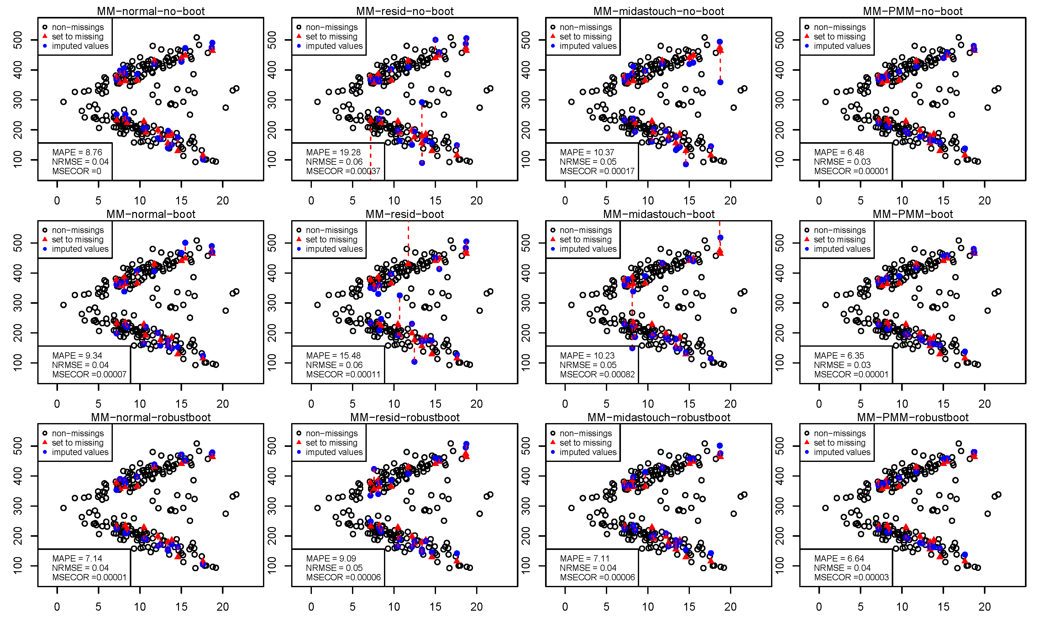
Figure 3 shows the results from using robust MM estimators. While model uncertainty is not considered for the first row of results in this figure, in the second and third rows of graphics, model uncertainty is considered by a bootstrap and a robust bootstrap.
Finding 5: Results generally improve when using a robust bootrap together with a robust MM estimator.
Finding 6: The best results are obtained by considering the imputation uncertainty with PMM. The combination of imputeRobust with robust bootrap, robust MM estimation, and PMM provides the best results.
Finding 7: For the imputation uncertainty by using the residuals, the (robustly) weighted and matched residuals through midastouch advance the results compared with the unweighted version.

3.2. Simulation Results

A synthetic data set with n = 200 data points is repeatedly simulated with 2000 repetitions. Multiple imputation methods such as MICE (PMM and midastouch), IRMI, imputation with XGBoost, and imputeRobust are carried out with 10 multiple imputations. The results are pooled using the pooling rule of Rubin [21]. The data generation procedure is as follows:
First n / 2 points are simulated, denoted as x, from a normal distribution N ( 200 , 40 ) , and sorted in increasing order. Generate the variable y = x + N ( 200 , 20 ) . Generate n / 2 points, denoted as x 2 , from N ( 200 , 40 ) , and sort them in decreasing order. Generate the variable y 2 = x 2 + N ( 400 , 20 ) . Create a data frame with three variables:
Price: 
Concatenation of y and y 2 (Price).
Age: 
Transformation of concatenation of x and x 2 by the formula x 10 10 (Age).
Type: 
A factor variable with “classic” for the first n / 2 points and “regular” for the rest. Figure 3, top left, shows one realization already including outliers as introduced below.
We introduce 30% missing values into the column Price based on a specified mechanism (kind) and at a specified proportion (rate). We select a random sample of rows with the MAR mechanism, where the probability of each row being selected is proportional to the Age value in that row. The modified dataframe with the newly introduced missing values in column P r i c e is returned.
To generate a data set of n ( o u t ) (non-representative) outliers each row is a random draw from a multivariate normal distribution. The mean vector of this distribution is fixed at c(300, 15) and the covariance matrix is 10 × 1 0.8 0.8 1 . Random noise is added to the first column of the dataframe. This noise is drawn from a normal distribution with mean 0 and standard deviation 20. Each outlier is then assigned a type, either “regular” or “classic”, with the intention to roughly equally randomly divide the outliers into these two categories. Figure 3, top left, shows one realization already including these outliers seen in the middle of the two data clouds.
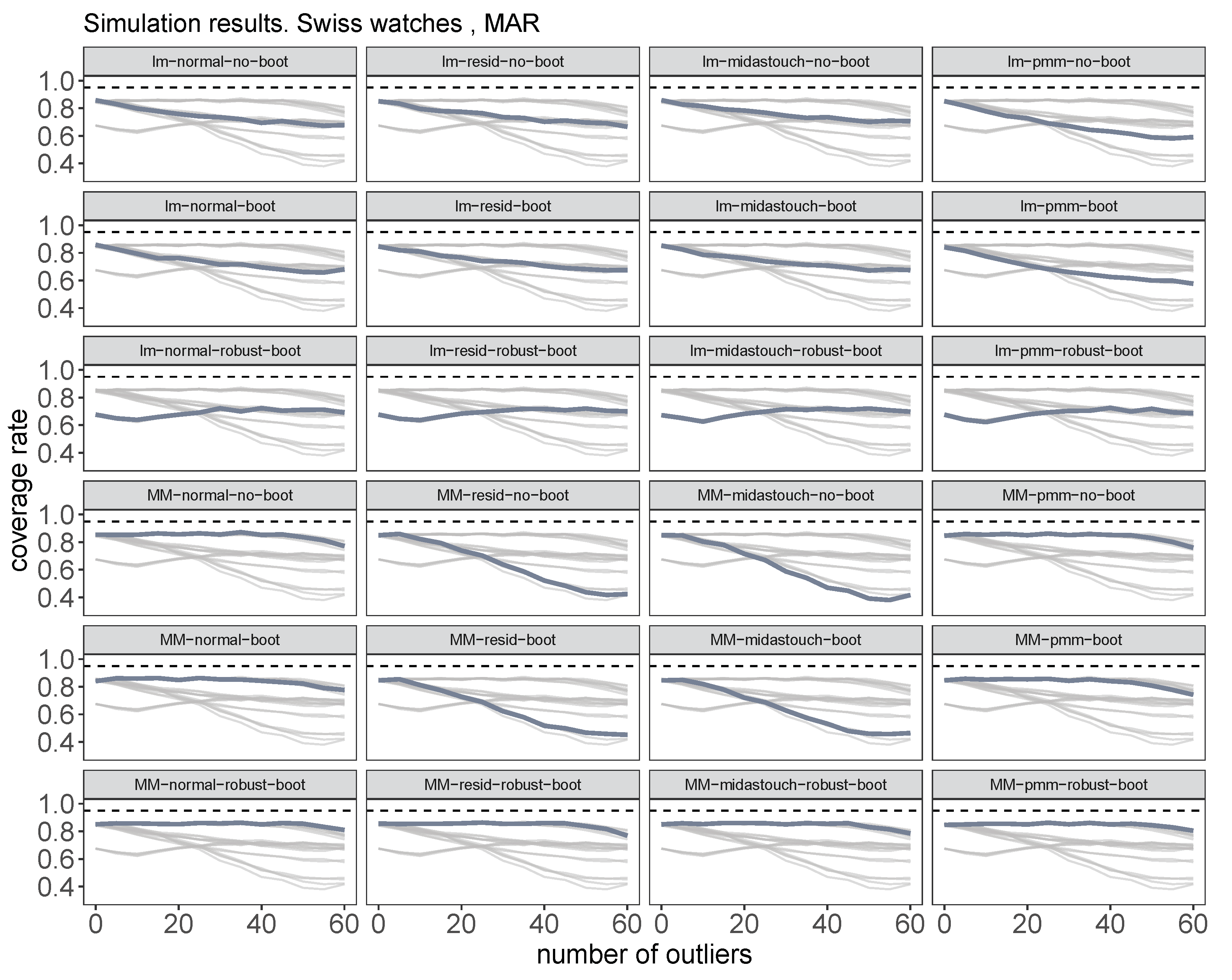
Figure 4 shows the coverage rates for the mean price of classic watches related to a significance level of 0.05 for the benchmarking methods. Thick gray lines correspond to the actual methods, while for comparison reasons all other methods are displayed in light gray lines. The coverage rates are generally below 0.95, whereby midastouch gives the most realistic ones, even for larger amounts of outliers. This is somehow surprising because this method is very sensitive to outliers [7]. Other methods—expect IRMI—are influenced by outliers.
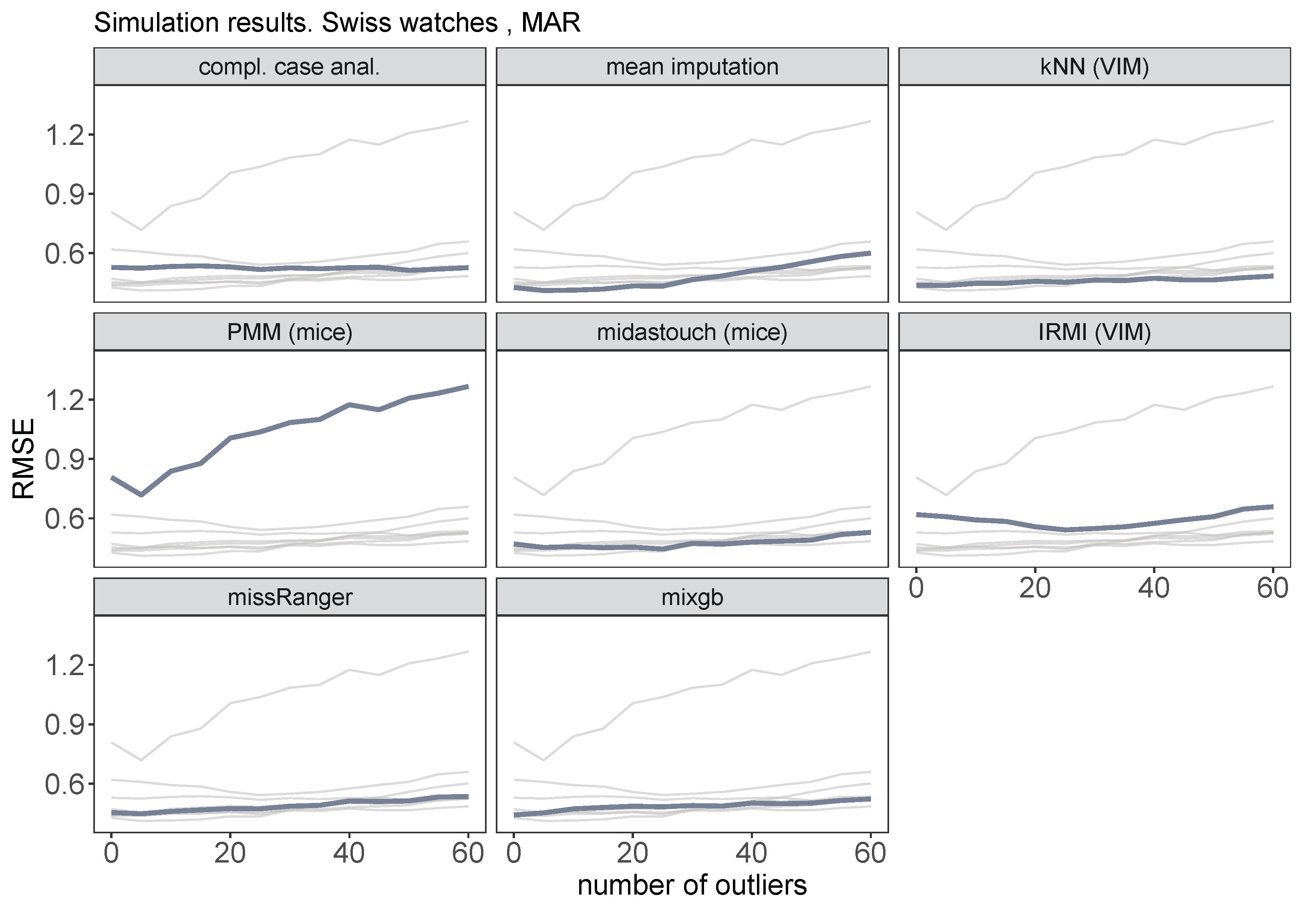
As one can see from Figure 5 that these methods involve some model misspecification by not considering the interaction term, mean imputation is competitive with sophisticated benchmarking model-based methods.
Figure 6 and Figure 7 show the coverage rates and RMSE for imputeRobust. Generally, one can see that both robust MM estimators and robust bootstrapping are necessary to stay robust against outliers (last line of graphics in this figure), especially for the residual and midastouch imputation uncertainty approaches.
Finding 8: For population data, MM regression with no bootstrap gives the best result for considering imputation uncertainty with normal error or PMM. It outperforms OLS regression and residual bootstrapping.
Finding 9: For sample data, taking model uncertainty into account, the combination of MM regression, robust bootstrap, and normal error or PMM to account for imputation uncertainty are the best choices. A robust bootstrap will not repair ordinary least-squares regression in terms of outliers. The robust bootstrap is preferable to the ordinary bootstrap.

3.3. Carbon Footprint

3.3.1. Carbon Footprint of the Simulations

All results were calculated on a MacBookPro M1 Max with 32 GB of RAM on macOS Ventura on 10 CPUs in parallel. We assume that the MacBook Pro consumes around 30 watts per hour under heavy load. The simulations took about 6 h of heavy computations on all 10 CPUs, that’s 180 watt-hours or 0.18 kilowatt-hours (kWh). Assuming the global average carbon footprint for electricity is about 475 g CO 2 per kWh as of the last update. Therefore, this is 0.18 kWh * 475 g CO 2 /kWh = 85.5 g CO 2 for 6 h of usage.

3.3.2. Carbon Footprint of imputeRobust

With the same equipment, for one imputation with imputeRobust of our data set with 200 observations, approx. 0.05 s on one CPU are needed for robust MM-regression with PMM, and about 0.03 s are needed in average for ordinary least squares estimation with normal noise. Any other method of imputeRobust lies between these two numbers.
To illustrate this, let’s make a very simplified assumption: if using all 10 CPUs corresponds to 100% power usage, then using 1 out of 10 CPUs might correspond to roughly 10% power usage. Again, this is an oversimplified assumption and actual power consumption will not scale linearly like this. If we assume the power consumption is 10%, we get 3 watts. If the calculations take 0.05 s, then the energy used is:
Energy (in watt-seconds, equivalent to joules) = Power (watts) × Time (seconds) = 3 W × 0.05 s = 0.15 joules.
To convert this to kilowatt-hours this is 0.15 joules = 0.00000004167 kWh.
Using
the same carbon intensity as before (475 g CO 2 per kWh):
0.00000004167 kWh * 475,000 g CO 2 /kWh = 0.0000198 g CO 2 , or 0.0198 mg CO 2 .
This is a very rough estimation, and actual figures can vary based on many factors. Furthermore, consider that Apple’s Silicon (like the M1 Max chip) is designed to be more energy-efficient than many other laptop processors, which could reduce energy consumption and thus carbon emissions.
Considering all assumptions, the carbon emission of one imputation of our data set with 200 observations on three variables and 30% of missing values in the response variable will be below 0.0000198 g CO 2 .

4. Discussion and Conclusions

4.1. General Comments

Several studies have shown the power of IRMI [6,7] and its usefulness and superior performance in practice when dealing with outliers in a data set. However, model uncertainty when imputing sample data can only be considered in IRMI when bootstrapping the data by hand before sending it to IRMI. While this would be easily be possible, a ordinary bootstrap is not the best choice and can undermine the robustness properties of a robust imputation method. The new algorithm, imputeRobust solves this issue by using a robust bootstrap, and as new enhancement various different imputation uncertainty procedures are provided. Last but not least, we allow to specify a complex statistical model for any variable in the data set to consider transformations of variables, the addition of quadratic or cubic terms or polynoms and interaction terms.

4.2. Concrete Findings

Our findings indicate that when handle missing data in a dataset, particularly when the data has outliers or requires complex modeling, the choice of imputation method can significantly affect the accuracy and robustness of the results.
The k-Nearest Neighbors (kNN) algorithm, as seen in Finding 1, was the standout performer among all the methods benchmarked in our study. It is notable that kNN was unaffected by outliers and offered superior accuracy. This underlines its reliability for imputing missing values, especially in scenarios characterized by data irregularities. kNN is not affected by model misspecification since it does not rely on a statistical model but only on distances between observations.
In contrast, as indicated by Findings 2 and 3, most of the other methods we analyzed were heavily impacted by outliers or incorrect model choice. This includes popular methods such as the Predictive Mean Matching (PMM) implementation in MICE [8], which has been claimed to be robust to model misspecification. Our findings suggest a re-evaluation of these claims may be in order. Even if the number of outliers is zero, imputeRobust outperforms benchmarking methods, such as IRMI and others, because it can pass complex models to the imputation algorithm to avoid model misspecifications.
Although imputation with random forests and XGBoost is robust against model misspecifications, it is influenced by outliers and thus gives lower coverage rates and a higher RMSE than imputeRobust.
In terms of methods for handling outliers, our Findings 4 and 5 show that a robust bootstrap can mitigate the influence of outliers, but not sufficiently in isolation. However, when paired with a robust MM estimator, the treatment of outliers significantly improves.
Our proposed algorithm, imputeRobust, as discussed in Finding 6, achieves the best results by incorporating a robust bootstrap, a robust MM estimator, and PMM to deal with imputation uncertainty. This points towards the necessity of a comprehensive, multi-pronged approach when dealing with outlier-robust imputation.
Addressing the issue of imputation uncertainty, as per Findings 7 to 9, the use of (robustly) weighted matched residuals (midastouch) improves outcomes compared with unweighted raw residuals. When considering population data, MM regression without bootstrap gives the best result for considering imputation uncertainty with normal error or PMM, outperforming OLS regression and residual bootstrap. For sample data, a combination of MM regression, robust bootstrap, and normal error or PMM to account for imputation uncertainty provides the most accurate results.
A key insight here is that a robust bootstrap does not repair ordinary least squares regression in terms of outliers, but it does offer superior performance to the ordinary bootstrap.

4.3. Conclusions

In conclusion, our results underscore the importance of careful method selection and the consideration of multiple factors, including the presence of outliers, model specification, and the nature of the data (i.e., population or sample data). They also provide strong evidence for the potential of our new algorithm, imputeRobust, to effectively handling missing data with robustness and precision.
The imputeRobust algorithm can handle different patterns of (multivariate) missingness, different amounts of missing values, and continuous, categorical, or binary variables. Furthermore, for each variable with missing parts, a complex model can be passed through the algorithm, allowing, for example, interactions between predictors or the use of transformations or polynomials. This is why it can be used for many different datasets. imputeRobust is implemented as a chain with an outer loop to update imputations until convergence.
The new algorithm imputeRobust for imputing missing values is valuable for a broad range of stakeholders. These primarily include data scientists, statisticians, and researchers across various fields such as healthcare, social sciences, economics, and more who regularly work with datasets that may have missing values. Additionally, industries that rely on accurate data analysis for decision-making, like finance, marketing, tech, and government agencies, are also key stakeholders. Even software developers creating data analysis tools could benefit from advancements in robust imputation techniques, as we presented in this article.
Finally, in order to reach a wider audience, imputeRobust will be made available on GitHub, more specifically on https://github.com/statistikat/VIM, accessed on 30 April 2023. This is to ensure that the information is accessible, understandable, and usable for those who can benefit from it. After being tested by interested users from all over the world, it will finally be made available on CRAN, the comprehensive R archive network, as part of the R package VIM [17].

4.4. Limitations

Basically, imputeRobust just assumes that you can provide a complex model that allows a linear relationship between the response and the predictor matrix for the majority of the data points. If this is not the case, a non-linear model using generalized additive models can also be used in imputeRobust. However, this has not been discussed in this paper.
Due to constraints on length, we’ve only explored one specific dataset and simulation. The selection was driven by the desire to illuminate particular issues inherent in a certain data context and further explore these issues through simulation. However, additional simulation studies could potentially yield further insights. Nonetheless, the current simulation has highlighted key points, contributing to the concise nature of this article.
Computational times are not reported in this study. For information regarding the computational times associated with MM-regression and least squares regression, we direct readers to the relevant original papers, as these methodologies typically consume the majority of computational time. Existing literature thoroughly documents the computation times of MM-regression and ordinary least squares regression. In cases of categorical variables with missing values, we recommend consulting the research by ref. [6]. This work delves into the computation times associated with the multinomial model, which, like imputeRobust, is used in the context of missing value imputation. It’s worth noting that [6] also reports on the computation times for IRMI for continuous variables, which are quite comparable to those of imputeRobust. This similarity is not surprising, given that the MM fit—the most computationally intensive part of both algorithms—is common to both methods.
Our simulations were based on a sample size of only 200 observations. Even though the results are good with a sample size of 200, they become better with larger data sets as more information becomes available, if the computational speed allows. It is worth mentioning that the methods discussed in this study have been found to be effective for large datasets encompassing many variables since the underlying regression and classification methods are proven to work for large data sets [22]. Thus, despite the study’s limitations, the presented techniques demonstrate substantial potential in the field of missing data imputation.
Nowadays, deep learning methods are heavily used in many applications, see e.g., refs. [23,24], and used for the imputation of missing values [25,26,27]. However, these artificial deep neural network-based methods are sensitive to outliers as the standard loss functions are not robust. Further work is needed to make these methods robust against outliers first.
The carbon footprint was estimated not only for the simulations but also for our new algorithm. More extensive evaluation might be useful since many factors influence the carbon footprint, such as the runtimes of imputeRobust on different sizes of data and the amount of missingness, and you would need to know the exact power consumption of your device and the carbon intensity of your local electricity supply.

Funding

This research received no external funding.

Data Availability Statement

The simulation of the data sets used is clearly described in Section 3.2.

Conflicts of Interest

The author declare no conflict of interest.

Abbreviations

The following abbreviations are used in this manuscript:
IRMIIterative Stepwise Robust Model-Based Imputation
kNNk nearest neighbor imputation
MICEMultiple Imputation with Chained Equations
PMMPredictive Mean Matching

Appendix A

Appendix A.1

Mean imputation is a simple and commonly used method to handle missing data. This algorithm replaces missing values in each variable with the mean value of the observed data for the same variable. The mean imputation algorithm can be described as follows:
Algorithm A1 Mean Imputation Algorithm (for benchmarking only).
1:
for each variable with missing data do
2:
    Calculate the mean of the observed values for the current variable.
3:
    Replace missing values in the current variable with the calculated mean.
4:
end for
Mean imputation offers a quick and easy way to handle missing data. However, it may not always be the best method, as it can lead to underestimated variances and biased estimates, especially when the data is not missing completely at random. More advanced methods like multiple imputation are often preferred for handling missing data in statistical analyses.
kNN imputation in the R package VIM REFERENCE uses Gower’s distance, which is suitable for mixed data that can include ordinal, continuous, and categorical variables.
Gower’s distance is particularly useful because it can handle different types of variables by converting each type of variable to a [0, 1] scale, then computes the distances as a sum of the scaled differences over all variables.
For each missing value in the dataset, the algorithm finds the k nearest observations based on the Gower’s distance. If there are k such neighbors, it then imputes the missing value: For continuous or ordinal data, it uses the mean value of the neighbors. For categorical data, it uses the mode (most common value) of the neighbors. If there are less than k neighbors available, the algorithm skips that missing value and moves to the next, see Algorithm A2.
Algorithm A2 kNN Imputation Algorithm using Gower’s Distance.
1:
procedure kNN( D a t a , k )
2:
    for each i where D a t a [ i ] is missing do
3:
         N e i g h b o r s the k points in D a t a with the smallest Gower’s distances to i that are not missing
4:
        if there are k such N e i g h b o r s  then
5:
           if  D a t a [ i ] is continuous or ordinal then
6:
                D a t a [ i ] median( N e i g h b o r s )
7:
           else if  D a t a [ i ] is categorical then
8:
                D a t a [ i ] mode( N e i g h b o r s )
9:
           end if
10:
       else
11:
           Continue to the next i
12:
        end if
13:
    end for
14:
    return  D a t a
15:
end procedure
Please note that the actual implementation in the VIM package is more complex as it handles different edge cases and is optimised in terms of performance.
Multiple Imputation by Chained Equations (MICE), also known as Fully Conditional Specification (FCS), is another popular method for handling missing data. This method works by performing multiple imputations for the missing values, creating several different complete datasets. The results from these datasets can then be pooled to create a single, more robust estimate. Algorithm A3 represents a simplified version of the MICE algorithm.
Algorithm A3 Multiple Imputation by Chained Equations (MICE).
1:
procedure MICE( D a t a , m , I t e r a t i o n s )
2:
    Initialize D a t a 1 , D a t a 2 , , D a t a m with simple imputations (e.g., mean imputation)
3:
    for  k = 1 to m do
4:
        for  i t e r = 1 to I t e r a t i o n s  do
5:
           for each variable V with missing values in D a t a k  do
6:
               Predict V given other variables using D a t a k (create a prediction model)
7:
               Replace missing values in V in D a t a k with predictions from the model
8:
           end for
9:
        end for
10:
    end for
11:
    return  D a t a 1 , D a t a 2 , , D a t a m
12:
end procedure
“Midastouch”, on the other hand, also fits a linear regression model to predict missing values but it modifies the selection criteria, see Algorithm A5 [18].
In the Multiple Imputation by Chained Equations (MICE) framework, for categorical variables, by default, the method used is Bayesian polytomous logistic regression. This method is suitable for categorical variables (both ordered and unordered).
The Bayesian polytomous logistic regression creates a probabilistic model for each category level and uses these probabilities to impute missing values. This approach accounts for the uncertainty of the imputed values and naturally handles the categorical nature of the variable.
The exact method might slightly differ based on the number of categories, order of categories (for ordinal data), and other factors. For example, for binary variables (a special case of categorical variables with two levels), the MICE algorithm uses logistic regression as a default.
Algorithm A4 MICE using Predictive Mean Matching (PMM).
1:
procedure MICE_PMM( D a t a , m , I t e r a t i o n s )
2:
    Initialize D a t a 1 , D a t a 2 , , D a t a m with simple imputations (e.g., mean imputation)
3:
    for  k = 1 to m do
4:
        for  i t e r = 1 to I t e r a t i o n s  do
5:
           for each variable V with missing values in D a t a k  do
6:
               Predict V given other variables using a linear regression model in D a t a k
7:
               For each missing value in V in D a t a k , find set S of observed values in V that are closest to the predicted value
8:
               Replace missing value with a random selection from set S
9:
           end for
10:
      end for
11:
   end for
12:
   return  D a t a 1 , D a t a 2 , , D a t a m
13:
end procedure
Algorithm A5 Midastouch Imputation.
1:
procedure Midastouch( D a t a , y )
2:
    Identify y o b s (observed values) and y m i s (missing values) in y in D a t a
3:
    Draw a bootstrap sample from the donor pool of y o b s , called y b s
4:
    Estimate a beta matrix on y b s using the leave one out principle
5:
    Compute type II predicted values for y o b s and y m i s using the beta matrix, producing predicted y o b s (nobs × 1) and predicted y m i s (nmis × nobs)
6:
    Calculate the distance between each predicted y o b s and the corresponding predicted y m i s
7:
    Convert the distances to drawing probabilities
8:
    for each missing value in y m i s  do
9:
        Draw a donor from the entire donor pool considering the drawing probabilities
10:
      Replace the missing value with the observed value of the selected donor in y
11:
    end for
12:
    return  D a t a
13:
end procedure
Random Forest is a powerful machine learning algorithm that can also be used for imputation of missing data. The R package ranger provides an efficient implementation of Random Forest, which can be used for imputation.
Algorithm A6 is a simplified version of the Random Forest imputation algorithm using ranger.
This approach takes advantage of the strengths of Random Forest, including its ability to handle non-linear relationships and interactions between variables.
Please note that in practice, additional steps might be necessary for tuning the Random Forest parameters (NumTrees and mTry), assessing the quality of the imputations, and handling different types of variables (continuous, ordinal, categorical).
Algorithm A6 Random Forest Imputation using Ranger.
1:
procedure missRanger( D a t a , N u m T r e e s , m T r y )
2:
    for each variable V with missing values in D a t a  do
3:
        Create a copy of D a t a , called D a t a C o p y
4:
        Replace missing values in V in D a t a C o p y with median(V) (or mode for categorical variables)
5:
        Build a Random Forest model with N u m T r e e s trees and m T r y variables tried at each split, using D a t a C o p y to predict V
6:
        Predict missing values in V in D a t a using the Random Forest model, and replace missing values with predictions
7:
    end for
8:
    return  D a t a
9:
end procedure

References

  1. Chapman, P.; Clinton, J.; Kerber, R.; Khabaza, T.; Reinartz, T.; Shearer, C.; Wirth, R. CRISP-DM 1.0 Step-by-Step Data Mining Guide; Technical Report; The CRISP-DM Consortium. 2000. Available online: https://www.kde.cs.uni-kassel.de/wp-content/uploads/lehre/ws2012-13/kdd/files/CRISPWP-0800.pdf (accessed on 30 May 2023).
  2. Vale, S. Generic Statistical Business Process Model, 2009. Joint UNECE/Eurostat/OECDWork Session on Statistical Metadata (METIS). Available online: https://unece.org/fileadmin/DAM/stats/documents/ece/ces/ge.61/2009/mtg1/zip.32.e.pdf (accessed on 30 May 2023).
  3. Rahm, E.; Do, H.H. Data Cleaning: Problems and Current Approaches. IEEE Data Eng. Bull. 2000, 23, 3–13. [Google Scholar]
  4. Mavrogiorgou, A.; Kiourtis, A.; Manias, G.; Kyriazis, D. Adjustable Data Cleaning Towards Extracting Statistical Information. Stud. Health Technol. Inform. 2021, 281, 1013–1014. [Google Scholar] [CrossRef] [PubMed]
  5. Brownlee, J. Data Preparation for Machine Learning: Data Cleaning, Feature Selection, and Data Transforms in Python; Machine Learning Mastery: San Juan, PR, USA, 2020. [Google Scholar]
  6. Templ, M.; Kowarik, A.; Filzmoser, P. Iterative stepwise regression imputation using standard and robust methods. Comput. Stat. Data Anal. 2011, 55, 2793–2806. [Google Scholar] [CrossRef]
  7. Templ, M. Imputation and Visualization of Missing Values; Springer International Publishing: Cham, Switzerland, 2023; p. 561. [Google Scholar]
  8. van Buuren, S. Flexible Imputation of Missing Data; CRC Press: Boca Raton, FL, USA, 2012. [Google Scholar] [CrossRef]
  9. Chambers, R.L. Outlier Robust Finite Population Estimation. J. Am. Stat. Assoc. 1986, 81, 1063–1069. [Google Scholar] [CrossRef]
  10. Filzmoser, P.; Gregorich, M. Multivariate Outlier Detection in Applied Data Analysis: Global, Local, Compositional and Cellwise Outliers. Math. Geosci. 2020, 52, 1049–1066. [Google Scholar] [CrossRef] [Green Version]
  11. Templ, M.; Gussenbauer, J.; Filzmoser, P. Evaluation of robust outlier detection methods for zero-inflated complex data. J. Appl. Stat. 2019, 47, 1144–1167. [Google Scholar] [CrossRef] [PubMed] [Green Version]
  12. van Buuren, S.; Groothuis-Oudshoorn, K. mice: Multivariate imputation by chained equations in R. J. Stat. Softw. 2011, 45, 1–67. [Google Scholar] [CrossRef] [Green Version]
  13. Salibián-Barrera, M.; Van Aelst, S.; Willems, G. Fast and robust bootstrap. Stat. Methods Appl. 2008, 17, 41–71. [Google Scholar] [CrossRef] [Green Version]
  14. Beaton, A.E.; Tukey, J.W. The Fitting of Power Series, Meaning Polynomials, Illustrated on Band-Spectroscopic Data. Technometrics 1974, 16, 147–185. [Google Scholar] [CrossRef]
  15. Rousseeuw, P.J.; Leroy, A.M. Robust Regression and Outlier Detection; John Wiley & Sons, Inc.: New York, NY, USA, 1987. [Google Scholar] [CrossRef] [Green Version]
  16. Venables, W.; Ripley, B. Modern Applied Statistics with S, 4th ed.; Springer: New York, NY, USA, 2002. [Google Scholar] [CrossRef]
  17. Kowarik, A.; Templ, M. Imputation with the R Package VIM. J. Stat. Softw. 2016, 74, 1–16. [Google Scholar] [CrossRef] [Green Version]
  18. Gaffert, P.; Meinfelder, F.; Bosch, V. Towards an MI-proper Predictive Mean Matching. In Proceedings of the Survey Research Methods Section, JSM 2018, Vancouver, BC, Canada, 28 July–2 August 2018. [Google Scholar]
  19. Mayer, M. missRanger: Fast Imputation of Missing Values. R package version 2.1.0. 2019. Comprehensive R Archive Network (CRAN). Available online: https://CRAN.R-project.org/package=missRanger (accessed on 30 May 2023).
  20. Deng, Y.; Lumley, T. Multiple Imputation Through XGBoost. arXiv 2023, arXiv:2106.01574. [Google Scholar] [CrossRef]
  21. Rubin, D. Multiple Imputation for Nonresponse in Surveys; John Wiley & Sons: Hoboken, NJ, USA, 2004; ISBN 0-471-65574-0. [Google Scholar] [CrossRef]
  22. Rousseeuw, P.; Van Driessen, K. Computing LTS regression for large data sets. Estadistica 2002, 54, 163–190. [Google Scholar] [CrossRef]
  23. Zeng, C.; Ma, C.; Wang, K.; Cui, Z. Predicting vacant parking space availability: A DWT-Bi-LSTM model. Phys. A Stat. Mech. Its Appl. 2022, 599, 127498. [Google Scholar] [CrossRef]
  24. Xiao, G.; Xiao, Y.; Ni, A.; Zhang, C.; Zong, F. Exploring influence mechanism of bikesharing on the use of public transportation—A case of Shanghai. Transp. Lett. 2023, 15, 269–277. [Google Scholar] [CrossRef]
  25. Templ, M. Artificial Neural Networks to Impute Rounded Zeros in Compositional Data. In Advances in Compositional Data Analysis: Festschrift in Honour of Vera Pawlowsky-Glahn; Filzmoser, P., Hron, K., Martín-Fernández, J., Palarea-Albaladejo, J., Eds.; Springer International Publishing: Cham, Switzerland, 2021; pp. 163–187. [Google Scholar] [CrossRef]
  26. Lubbe, S.; Templ, M.; Filzmoser, P. Comparison of Zero Replacement Strategies for Compositional Data with Large Numbers of Zeros. Chemom. Intell. Lab. Syst. 2021, 215, 104248. [Google Scholar] [CrossRef]
  27. Templ, M. Can the Compositional Nature of Compositional Data Be Ignored by Using Deep Learning Approaches? In Studies in Theoretical and Applied Statistics; Salvati, N., Perna, C., Marchetti, S., Chambers, R., Eds.; Springer: Cham, Switzerland, 2023; pp. 151–166. [Google Scholar] [CrossRef]
Figure 1. Imputation of the Swiss watches data set using selected benchmarking methods.
Mathematics 11 02729 g001
Figure 2. Imputation of the Swiss watches data set using imputeRobust with different parameters. Results are based on OLS regression.
Mathematics 11 02729 g002
Figure 3. Imputation of the Swiss watches data set using imputeRobust with different parameters. Results are based on MM-estimation.
Mathematics 11 02729 g003
Figure 4. Coverage rates for the mean price of classic watches for different number of outliers from 0 to 60. Benchmarking methods.
Mathematics 11 02729 g004
Figure 5. Root mean squared error for the mean price of classic watches for different number of outliers from 0 to 60.
Mathematics 11 02729 g005
Figure 6. Coverage rates for the mean price of classic watches for different number of outliers from 0 to 60. The new imputeRobust algorithm with different choices of parameters.
Mathematics 11 02729 g006
Figure 7. Root mean squared error for the mean price of classic watches for different number of outliers from 0 to 60. The new imputeRobust algorithm with different choices of parameters.
Mathematics 11 02729 g007
Table 1. Benchmarking methods.
MethodShort DescriptionReference
kNNk nearest neighbor imputation[17]
PMMPredictive mean matching using MICE[12]
midastouchAlmost PMM, but with another selection criteria[18]
ranger(Multiple) Imputation with random forests[19]
XGBoost(Multiple) Imputation with XGBoost[20]
IRMIIterative stepwise regression imputation using robust methods[6]
compl. case anal.Removing observations with missing values.
mean imputationImputation with the arithmetic mean of observed values.
Table 2. Settings for imputeRobust for lm- and MM-. lm symbolizes the use of ordinary least squares regression while MM denotes the using robust MM-regression estimators.
MethodModel UncertaintyImputation Uncertainty
-normal-no-bootnonormal noise
-resid-no-bootnoresidual noise
-midastouchno-bootnomidastouch
-pmm-no-bootnoPMM
-normal-boot/-normal-robustbootbootstap/robust bootstrapnormal noise
-resid-boot/-resid-robustbootbootstap/robust bootstrapresidual noise
-midastouch-boot/-wresid-robustbootbootstap/robust bootstrapmidastouch
-pmm-boot/-pmm-robustbootbootstap/robust bootstrapPMM
Disclaimer/Publisher’s Note: The statements, opinions and data contained in all publications are solely those of the individual author(s) and contributor(s) and not of MDPI and/or the editor(s). MDPI and/or the editor(s) disclaim responsibility for any injury to people or property resulting from any ideas, methods, instructions or products referred to in the content.