The Longest (s, t)-Path Problem on O-Shaped Supergrid Graphs

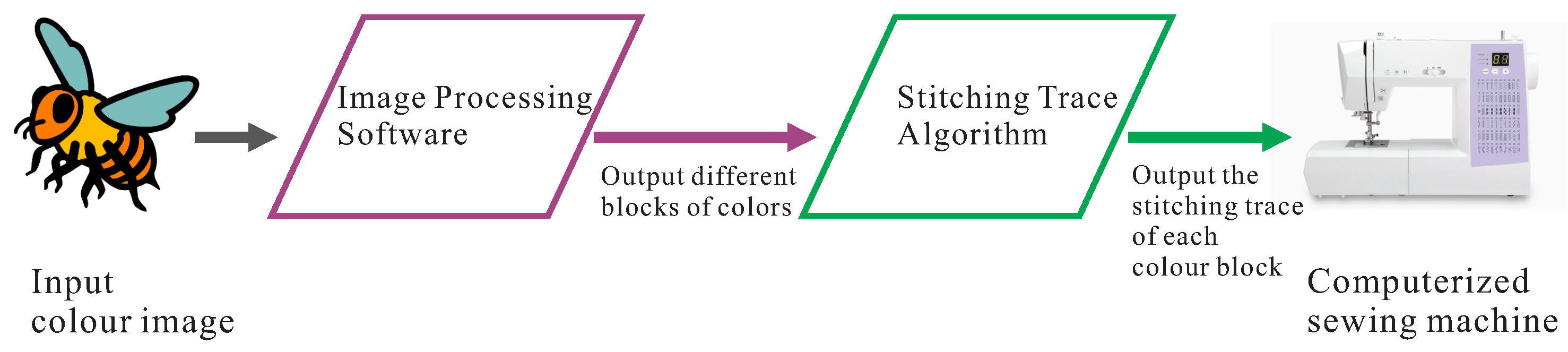
Abstract

The longest $(s,t)$-path problem on supergrid graphs is known to be NP-complete. However, the complexity of this problem on supergrid graphs with or without holes is still unknown.In the past, we presented linear-time algorithms for solving the longest $(s,t)$-path problem on L-shaped and C-shaped supergrid graphs, which form subclasses of supergrid graphs without holes. In this paper, we will determine the complexity of the longest $(s,t)$-path problem on O-shaped supergrid graphs, which form a subclass of supergrid graphs with holes. These graphs are rectangular supergrid graphs with rectangular holes. It is worth noting that O-shaped supergrid graphs contain L-shaped and C-shaped supergrid graphs as subgraphs, but there is no inclusion relationship between them. We will propose a linear-time algorithm to solve the longest $(s,t)$-path problem on O-shaped supergrid graphs. The longest $(s,t)$-paths of O-shaped supergrid graphs have applications in calculating the minimum trace when printing hollow objects using computer embroidery machines and 3D printers.

1. Introduction

All graphs considered in this paper are undirected and simple. Let G be a graph. We denote the vertex set and the edge set of G by $V\left(G\right)$ and $E\left(G\right)$, respectively. A Hamiltonian path (resp., cycle) on graph G is a simple path (resp., cycle) that visits every vertex of G exactly once. The Hamiltonian path (cycle) problem involves determining whether a graph has a Hamiltonian path (cycle). A Hamiltonian $(s,t)$-path is a Hamiltonian path in a graph that starts from vertex s and ends at vertex t. A graph is Hamiltonian-connected if it contains a Hamiltonian $(s,t)$-path for every two distinct vertices $s,t$ in the graph. The longest $(s,t)$-path in a graph is the path from s to t that visits the most vertices. The longest $(s,t)$-path problem on a graph involves determining whether the graph contains a Hamiltonian $(s,t)$-path and finding the longest $(s,t)$-path if it is not. The above problems are NP-complete for general graphs [1,2], as well as for various special graph classes, including undirected path graphs [3], circle graphs [4], split graphs [5], triangular grid graphs [6], supergrid graphs [7], bipartite graphs [8], grid graphs [9], and so on. Next, we will discuss the conditions under which a Hamiltonian $(s,t)$-path does not exist. Let G be a connected graph and $V_1\subseteq V\left(G\right)$. We say that $V_1$ is a vertex cut if removing $V_1$ from G results in a disconnected graph. Moreover, a vertex $v\in V\left(G\right)$ is called a cut vertex if removing v from G makes it disconnected [10]. Let us consider that s is a cut vertex of G. Then, removing s from G results in some disjoint connected components. Since a Hamiltonian path from s to t must pass through all vertices of G exactly once and the path from s to other components must pass through s at least twice, a Hamiltonian $(s,t)$-path does not exist. The same holds true for t. In addition, a Hamiltonian $(s,t)$-path does not exist when $\{s,t\}$ is a vertex cut of G using similar arguments. Thus, if s or t is a cut vertex of G or if $\{s,t\}$ is a vertex cut of G, then graph G contains no Hamiltonian $(s,t)$-path.

Supergrid graphs are proposed to solve the calculation of stitch paths on computer embroidery machines [7]. If we input a colored picture, computer image software first processes it into blocks of different colors; then, the stitch algorithm calculates each stitch path in every block and transfers it to the computerized embroidery machine for embroidery work. Figure 1 shows the operation flow of a computerized embroidery machine. The supergrid graph is mainly used in the calculation of the stitch path. Considering the operation of computer embroidery machines, each needle point is an integer coordinate, and its moving direction includes its eight directions: up, down, left, right, upper-left, upper-right, upper-left, and lower-left. We can express each needle point as a lattice, as shown in Figure 2a, and the eight adjacent lattices are the next possible positions where the needle point may move to, so we can represent the lattice as a vertex of the graph, and there are edge adjacencies among them. Figure 2b is a graph representation of Figure 2a. Then, the block generated by each image software is a supergrid graph. The supergrid graph is then defined as follows: each vertex v with integer coordinates is represented as $(v_x,v_y)$, where $v_x$ and $v_y$ are the x- and y-coordinates of v, respectively. In the graphical representations in this paper, we use $(1,1)$ as the coordinates of the uppermost left vertex of a supergrid graph. For two vertices u and v of a supergrid graph, $(u,v)$ is an edge if and only if $|u_x-v_x|⩽1$ and $|u_y-v_y|⩽1$. In other words, u is one of the following vertices: $(v_x,v_y-1)$, $(v_x,v_y+1)$, $(v_x-1,v_y-1)$, $(v_x-1,v_y)$, $(v_x-1,v_y+1)$, $(v_x+1,v_y-1)$, $(v_x+1,v_y)$, or $(v_x+1,v_y+1)$. Supergrid graphs include grid graphs and triangular grid graphs as subgraphs. Although they have an identical set of vertices, their edge sets are entirely distinct. Therefore, these graph classes do not belong to each other; that is, a supergrid graph is not necessary a grid graph or a triangular grid graph, and vice versa. Clearly, grid graphs are bipartite and planar [9], but triangular grid and supergrid graphs are not always bipartite or planar.

Figure 1. The primary elements and operational sequence of a computerized embroidery procedure.

Figure 2. (a) A collection of lattices and (b) the associated supergrid graph of (a), in which each lattice is represented as a vertex with integer coordinates.

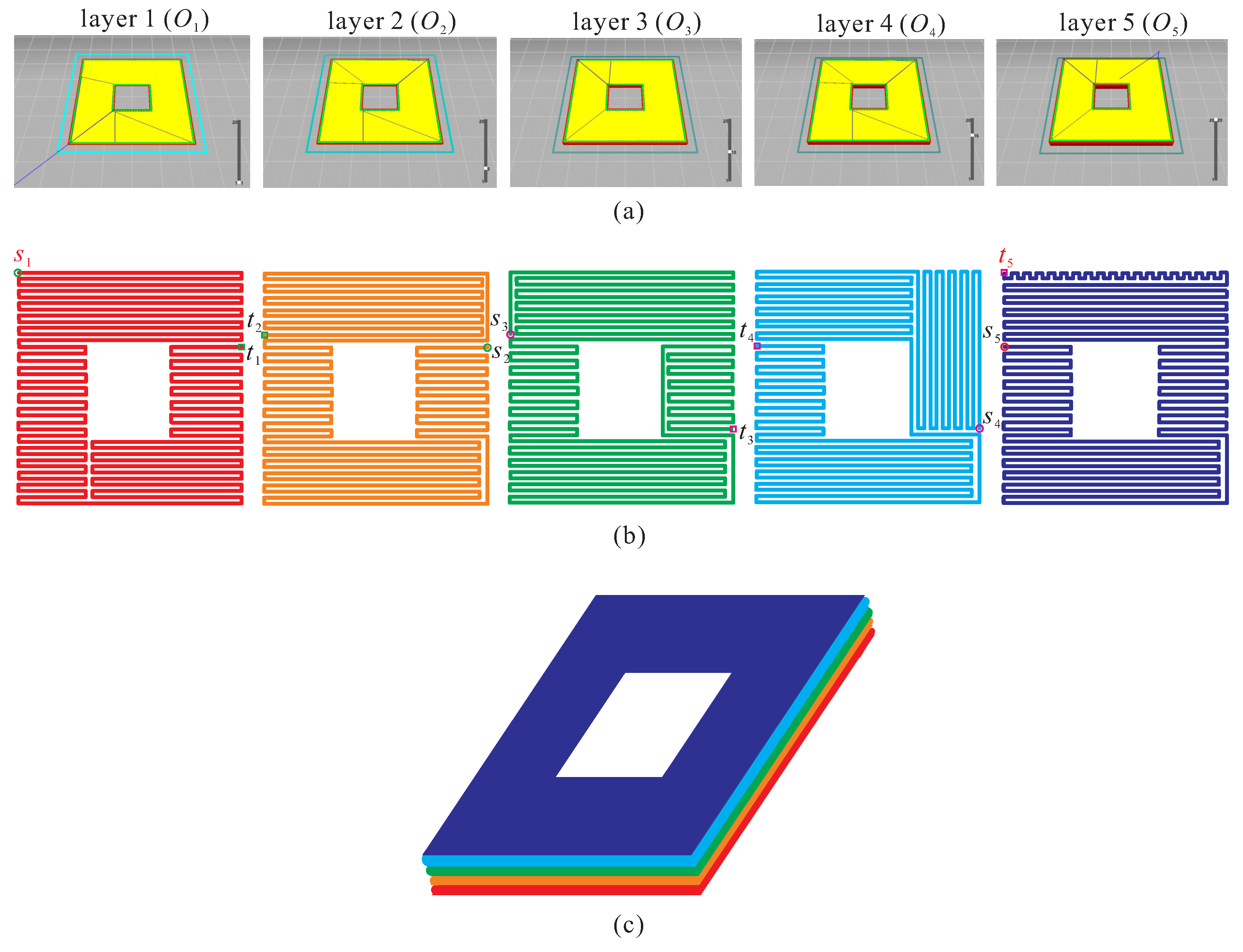
The Hamilton path problem on supergrid graphs is known to be NP-complete [7]; hence, the longest $(s,t)$-path problem is also NP-complete for supergrid graphs. However, these two problems for supergrid graphs with or without holes are still open. This paper proposes a linear-time algorithm to solve the longest $(s,t)$-path problem on O-shaped supergrid graphs, which are a subclass of hollow supergrid graphs. A preliminary version of this paper has appeared in [11], and a preprint version of the paper has been posted on the arXiv system [12], an open platform for scholarly research exchange. The related research works are introduced as follows: Recently, Hamiltonian path (cycle) and Hamiltonian-connected problems for grid, triangular grid, and supergrid graphs have received much attention. Itai et al. [9] showed that Hamiltonian path and cycle problems for grid graphs are NP-complete and gave necessary and sufficient conditions for rectangular grid graphs to be Hamiltonian-connected. Zamfirescu et al. [13] provided sufficient conditions for a grid graph to have a Hamiltonian cycle and showed that all grid graphs of positive width have Hamiltonian line graphs. Chen et al. [14] improved the Hamiltonian path algorithm for rectangular grid graphs and presented a parallel algorithm for the Hamiltonian path problem with two given end vertices. Lenhart and Umans [15] showed that the Hamiltonian cycle problem on solid grid graphs can be solved in polynomial time. In addition to grid graphs, researchers have studied Hamiltonian cycle and path problems on triangular and hexagonal grid graphs, as well as alphabet grid graphs. Keshavarz-Kohjerdi and Bagheri [16] presented a linear-time algorithm for computing the longest $(s,t)$-paths in L-shaped grid graphs. Recently, Nishat et al. [17] designed a linear-time algorithm to reconfigure any 1-complex $s,t$ Hamiltonian path to a canonical Hamiltonian path in rectangular grids. Supergrid graphs, a more complex type of graph, have also been studied. Hung et al. [7] proved that Hamiltonian cycle and path problems on supergrid graphs are NP-complete, while showing that every rectangular supergrid graph is Hamiltonian. In subsequent studies, researchers explored the complexities of Hamiltonian problems for special subclasses of supergrid graphs, such as linear-convex [18] and rectangular supergrid graphs [19]. In [20,21], we presented linear-time algorithms for solving the longest $(s,t)$-path problem on L-shaped and C-shaped supergrid graphs, which form two subclasses of supergrid graphs without holes. In this paper, we study the Hamiltonian and longest $(s,t)$-path problems for O-shaped supergrid graphs, which are rectangular supergrid graphs with rectangular holes. We prove that O-shaped supergrid graphs are always Hamiltonian and Hamiltonian-connected except for a few conditions and present a linear-time algorithm to compute the longest $(s,t)$-path under these exceptional conditions. This study can be regarded as the first attempt to solve the Hamiltonian and longest $(s,t)$-path problems on supergrid graphs with holes.

The Hamiltonian connectivity of O-shaped supergrid graphs can also be applied to compute the minimum trace of 3D printers as follows [11]: Let us consider a 3D printer with a hollow object (O-type object) being printed. The software produces a series of thin layers, designs a path for each layer, combines these paths of produced layers, and transmits the above paths to the 3D printer. Because 3D printing is performed layer by layer (see Figure 3a), each layer can be considered as an O-shaped supergrid graph. Let us suppose that there are k layers under the above 3D printing. If the Hamiltonian connectivity of O-shaped supergrid graphs holds true, then we can find a Hamiltonian $(s_i,t_i)$-path of an O-shaped supergrid graph $O_i$, where $O_i$, $1⩽i⩽k$, represents a layer under 3D printing. Thus, we can design an optimal trace for the above 3D printing, where $t_i$ is adjacent to $s_{i+1}$ for $1⩽i⩽k-1$. In this application, we restrict the 3D printer nozzle to be located at integer coordinates. As an example, Figure 3a shows the five layers, $O_1$–$O_5$, of a 3D print for an O-type object, and Figure 3b depicts the Hamiltonian $(s_i,t_i)$-paths of $O_i$ for $1⩽i⩽5$; the result of this 3D printing is shown in Figure 3c.

Figure 3. (a) The five layers ($O_1$–$O_5$) of a 3D printing model for an O-type object, (b) the computation of the Hamiltonian $(s_i,t_i)$-path for each layer $O_i$ shown in (a), and (c) the final result after completing the 5-layered 3D printing process.

The following is the organization of the paper: Section 2 introduces notations, observations, and previously established results, along with verification of the Hamiltonicity of O-shaped supergrid graphs. In Section 3, conditions are discovered that prohibit the existence of Hamiltonian $(s,t)$-paths in O-shaped supergrid graphs. Section 4 presents that O-shaped supergrid graphs are Hamiltonian-connected except for the conditions mentioned in Section 3. An algorithm for computing the longest $(s,t)$-paths of O-shaped supergrid graphs in linear time is described in Section 5. Finally, conclusions are provided in Section 6.

2. Notations and Background Results

This section introduces several terms and symbols, along with the presentation of some prior observations and established results related to the Hamiltonicity and Hamiltonian connectivity of rectangular supergrid graphs. For any graph-theoretic terminology that is not defined in this paper, please refer to [10].

Let G be a finite, undirected, and simple graph. Let $S\subseteq V\left(G\right)$ and $u,v\in V\left(G\right)$. The subgraph of G induced by S is denoted by $G\left[S\right]$, while the subgraph induced by $V\left(G\right)-S$ is denoted by $G-S$. We use $G-v$ to represent $G-\left\{v\right\}$ in general. If $(u,v)\in E\left(G\right)$, we say that u is adjacent to v and that u and v are incident to edge $(u,v)$. We use $u\sim v$ to indicate that u and v are adjacent and $u\nsim v$ to indicate that they are not adjacent. An edge $(u,v)$ is adjoined by a vertex w if $w\sim u$ and $w\sim v$. Two edges, $e_1=(u_1,v_1)$ and $e_2=(u_2,v_2)$, are said to be parallel and are denoted by $e_1\approx e_2$, if $u_1\sim u_2$ and $v_1\sim v_2$. A vertex adjacent to vertex v is called a neighbor of v. The set of neighbors of v in G is denoted by $N_G\left(v\right)$, and the set of neighbors along with v itself is denoted by $N_G\left[v\right]=N_G\left(v\right)\cup \left\{v\right\}$. The degree of vertex v in G, denoted by $de{g}_G\left(v\right)$, is the number of vertices adjacent to v. A path P of length $\left|P\right|$ in G, denoted by $v_1\to v_2\to \cdots \to v_{\left|P\right|-1}\to v_{\left|P\right|}$, is an ordered sequence of vertices $(v_1,v_2,\cdots ,v_{\left|P\right|-1},v_{\left|P\right|})$, such that $(v_i,v_{i+1})\in E\left(G\right)$ for $1⩽i<\left|P\right|$, and all vertices except $v_1,v_{\left|P\right|}$ in the sequence are distinct. The first and last vertices visited by P are denoted by $start\left(P\right)$ and $end\left(P\right)$, respectively. We use $v_i\in P$ to indicate that P visits vertex $v_i$, and $(v_i,v_{i+1})\in P$ to represent that P visits edge $(v_i,v_{i+1})$. A path from $v_1$ to $v_k$ is denoted by $(v_1,v_k)$-path. Additionally, we use P to refer to the set of vertices visited by path P if it is clear from the context. A cycle is a path C with $\left|V\right(C\left)\right|⩾3$ and $start\left(C\right)=end\left(C\right)$. Two paths (or cycles), $P_1$ and $P_2$, in graph G are vertex disjoint if $V\left(P_1\right)\cap V\left(P_2\right)=\varnothing$. If $end\left(P_1\right)\sim start\left(P_2\right)$, then two vertex-disjoint paths $P_1$ and $P_2$ can be concatenated into a path, which is denoted by $P_1\Rightarrow P_2$.

A two-dimensional supergrid, denoted by $S^{\infty }$, is an infinite graph with vertices corresponding to all points (vertices) in the plane with integer coordinates. Two vertices in $S^{\infty }$ are adjacent if and only if the difference between their x- or y-coordinates is, at most, 1. A supergrid graph is a finite vertex-induced subgraph of $S^{\infty }$. Each vertex v in a supergrid graph can be represented as $(v_x,v_y)$, where $v_x$ and $v_y$ are the x- and y-coordinates of v, respectively. The set of possible adjacent vertices of a vertex $v=(v_x,v_y)$ in a supergrid graph includes $(v_x,v_y-1)$, $(v_x,v_y+1)$, $(v_x-1,v_y-1)$, $(v_x-1,v_y)$, $(v_x-1,v_y+1)$, $(v_x+1,v_y-1)$, $(v_x+1,v_y)$, and $(v_x+1,v_y+1)$. An edge $(u,v)$ is called horizontal (resp., vertical) if $u_y=v_y$ (resp., $u_x=v_x$), and it is said to be crossed if it is neither horizontal nor vertical. Next, we define some special supergrid graphs studied in the paper, as follows.

Definition 1.

Graph $R(m,n)$ is a supergrid graph with vertex set $V\left(R\right(m,n\left)\right)$ consisting of all vertices of the form $v=(v_x,v_y)$, with $1⩽v_x⩽m$ and $1⩽v_y⩽n$. A supergrid graph is called a rectangular supergrid graph if it is isomorphic to $R(m,n)$ for some positive integers m and n. When $R(m,n)$ is considered, it is called an n-rectangle.

For $m,n⩾2$, a rectangular supergrid graph $R(m,n)$ contains four boundaries, each consisting of boundary edges. A path that visits all vertices and edges of a single boundary in $R(m,n)$ and that has a length equal to the number of visited vertices is called a boundary path. A vertex $v=(v_x,v_y)$ in $R(m,n)$ is called the upper-left (resp., upper-right, down-left, and down-right) corner, if for any vertex $w=(w_x,w_y)\in R(m,n)$, $w_x⩾v_x$, and $w_y⩾v_y$ (resp., $w_x⩽v_x$ and $w_y⩾v_y$, $w_x⩾v_x$ and $w_y⩽v_y$, and $w_x⩽v_x$ and $w_y⩽v_y$). In this paper, we assume that $(1,1)$ are the coordinates of the vertex in the upper-left corner in all figures, unless explicitly stated otherwise.

Definition 2.

Let us suppose that $R(m,n)$ is a rectangular supergrid graph. We define $L(m,n;k,l)$ as the supergrid graph obtained from $R(m,n)$ by removing the subgraph $R(k,l)$ located in the upper-right corner with coordinates $(m,1)$. An L-shaped supergrid graph is a supergrid graph isomorphic to $L(m,n;k,l)$ (see Figure 4a).

Figure 4. The structures of three types of supergrid graphs: (a) L-shaped supergrid graph $L(m,n;k,l)$, (b) C-shaped supergrid graph $C(m,n;k,l;c,d)$, and (c) O-shaped supergrid graph $O(m,n;k,l;a,b,c,d)$.

Definition 3.

Let $R(m,n)$ be a rectangular supergrid graph. We define a C-shaped supergrid graph $C(m,n;k,l;c,d)$ as a subgraph of $R(m,n)$ obtained by removing the subgraph $R(k,l)$ located at the vertex with coordinates $(m,c+1)$. Additionally, $R(m,n)$ and $R(k,l)$ must have exactly one border side in common, and we require that $m⩾2$, $n⩾3$, $k,l,c,d⩾1$ and $n=c+d+l$ (see Figure 4b).

Definition 4.

Let us consider a rectangular supergrid graph $R(m,n)$. An O-shaped supergrid graph $O(m,n;k,l;a,b,c,d)$ is obtained by removing subgraph $R(k,l)$ from vertex $(m-b,c+1)$ of $R(m,n)$. Graphs $R(m,n)$ and $R(k,l)$ do not share any border side. Parameters $m,n,k,l,a,b,c,d$ satisfy $m,n⩾3$, $k,l,a,b,c,d⩾1$, $m=a+b+k$ and $n=c+d+l$ (see Figure 4c).

When proving our results, it is necessary to partition a supergrid graph G into k disjoint parts, where $k⩾2$. We define such an operation on G as follows.

Definition 5.

Let us consider a supergrid graph G. A separation operation on G is a partition of G into k vertex-disjoint supergrid subgraphs $G_1$, $G_2$, ⋯, $G_k$, i.e., $V\left(G\right)=V\left(G_1\right)\cup V\left(G_2\right)\cup \cdots \cup V\left(G_k\right)$ and $V\left(G_i\right)\cap V\left(G_j\right)=\varnothing$ for $i\ne j$ and $1⩽i,j⩽k$, where $k⩾2$. A separation is referred to as vertical if it comprises a set of horizontal edges and as horizontal if it comprises a set of vertical edges.

Let $(G,s,t)$ be a supergrid graph G with two distinct specified vertices s and t. We assume without loss of generality that $s_x⩽t_x$ for the remainder of the paper, unless we explicitly state otherwise. We denote a Hamiltonian path between s and t in G as $HP(G,s,t)$. If a Hamiltonian $(s,t)$-path exists in G, we say that $HP(G,s,t)$ exists. In the following, we present some previously established results.

Let $R(m,n)$ be a rectangular supergrid graph with dimensions $m⩾n⩾2$. Let us consider a cycle $\mathcal{C}$ of $R(m,n)$, and let H be a boundary of $R(m,n)$, which is a subgraph of $R(m,n)$. We denote the restriction of $\mathcal{C}$ to H by ${\mathcal{C}}_{|H}$. If $|{\mathcal{C}}_{|H}|=1$, i.e., ${\mathcal{C}}_{|H}$ is a boundary path on H, ${\mathcal{C}}_{|H}$ is referred to as a flat face on H. If $|{\mathcal{C}}_{|H}|>1$ and ${\mathcal{C}}_{|H}$ contains at least one boundary edge of H, then ${\mathcal{C}}_{|H}$ is called a concave face on H. A Hamiltonian cycle of $R(m,3)$ is said to be canonical if it contains three flat faces on two shorter boundaries and one longer boundary, and one concave face on the other boundary, where the shorter boundary consists of three vertices. For $n=2$ or $n⩾4$, a Hamiltonian cycle of $R(m,n)$ is referred to as canonical if it contains three flat faces on three boundaries and one concave face on the other boundary. The following lemma shows the result from [7] that verifies the Hamiltonicity of rectangular supergrid graphs.

Lemma 1

(See [7]). The following statements are true for rectangular supergrid graph $R(m,n)$, where $m⩾n⩾2$:

$\left(1\right)$ If $n=3$, then $R(m,3)$ has a Hamiltonian cycle that is canonical.

$\left(2\right)$ If $n=2$ or $n⩾4$, $R(m,n)$ contains four canonical Hamiltonian cycles, with each having a concave face on a different boundary.

In Section 1 and in [19], we verified that if s or t is a cut vertex of $R(m,n)$, or if $\{s,t\}$ is a vertex cut of $R(m,n)$, then $HP\left(R\right(m,n),s,t)$ does not exist. Thus, $HP\left(R\right(m,n),s,t)$ does not exist if the following condition is satisfied:

(F1)

s or t is a cut vertex of $R(m,n)$, or $\{s,t\}$ is a vertex cut of $R(m,n)$ (see Figure 5a,b).

Figure 5. Rectangular supergrid graphs in which there is no Hamiltonian $(s,t)$-path for (a) $R(m,1)$ and (b) $R(m,2)$, where solid lines indicate the longest path between s and t.

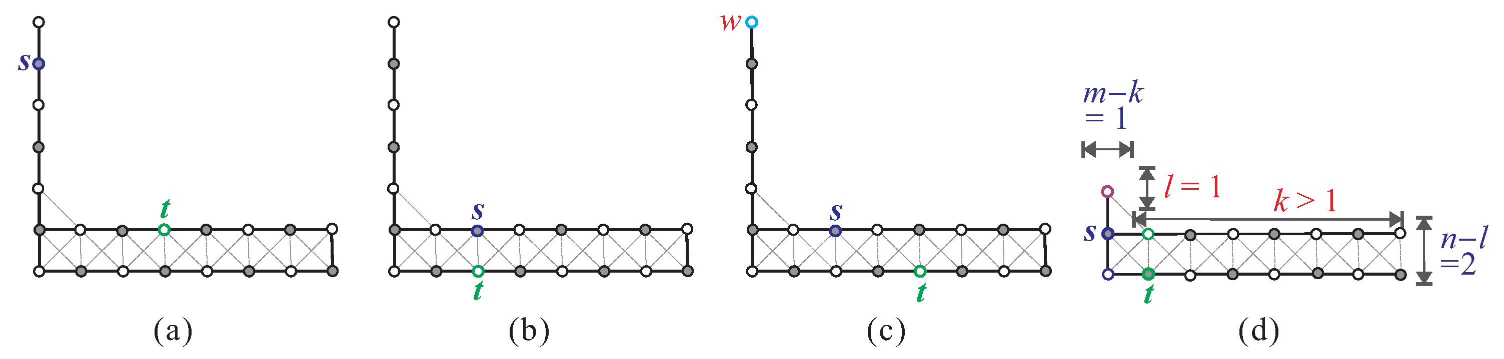
We demonstrated in [20] that in addition to condition (F1) (shown in Figure 6a,b), $HP\left(L\right(m,n;k,l),s,t)$ does not exist when any of the following conditions are satisfied.

Figure 6. L-shaped supergrid graph $L(m,n;k,l)$ does not contain a Hamiltonian $(s,t)$-path when one of the following conditions are satisfied: (a) s is a cut vertex; (b) $\{s,t\}$ is a vertex cut; (c) there exists a vertex w such that $de{g}_{L(m,n;k,l)}\left(w\right)=1$, $w\ne s$, and $w\ne t$; (d) $m-k=1$, $n-l=2$, $l=1$, $k⩾2$, and $\{s,t\}=\left\{\right(1,2),(2,3\left)\right\}$.

(F2)

For an L-shaped supergrid graph G, there exists a vertex $w\in G$, such that $de{g}_G\left(w\right)=1$, $w\ne s$, and $w\ne t$ (see Figure 6c).

(F3)

$m-k=1$, $n-l=2$, $l=1$, $k⩾2$, and $\{s,t\}=\left\{\right(1,2),(2,3\left)\right\}$ or $\left\{\right(1,3),(2,2\left)\right\}$ (see Figure 6d).

In addition to conditions (F1) and (F2) depicted in Figure 7a–c, respectively, we demonstrated in [21] that the existence of a Hamiltonian $(s,t)$-path in $C(m,n;k,l;c,d)$ is prohibited if $\left(C\right(m,n;k,l;c,d),s,t)$ satisfies any of the following conditions.

Figure 7. C-shaped supergrid graphs in which there is no Hamiltonian $(s,t)$-path, when one of the following conditions are satisfied: (a) s is a cut vertex; (b) $\{s,t\}$ is a vertex cut; (c) there exists a vertex w such that $de{g}_{C(m,n;k,l;c,d)}\left(w\right)=1$, $w\ne s$, and $w\ne t$; (d) $m=3$, $a=m-k=2$, $c=1$, and $\{s,t\}=\left\{\right(1,1),(2,2\left)\right\}$; (e–g) condition (F5) holds; (h) $a=m-k=1$ and $s_y,t_y>c+l$.

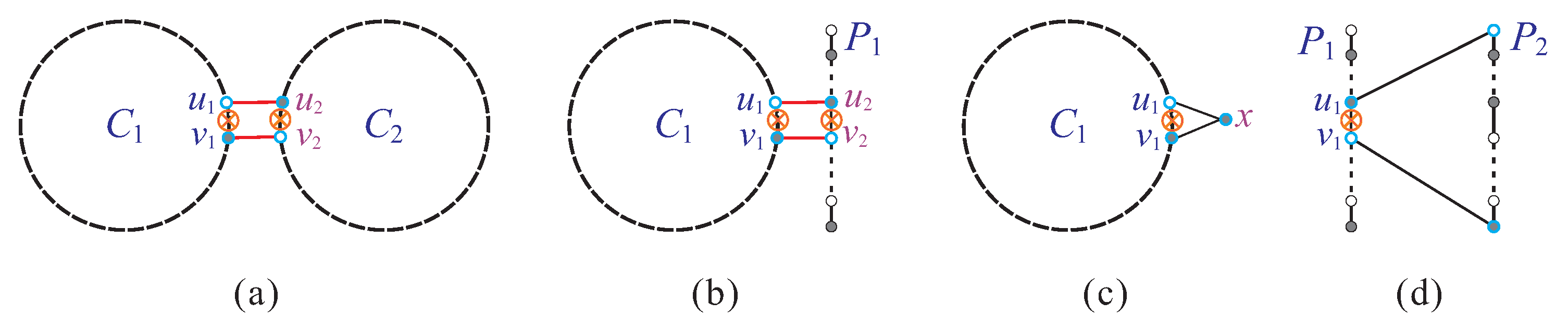
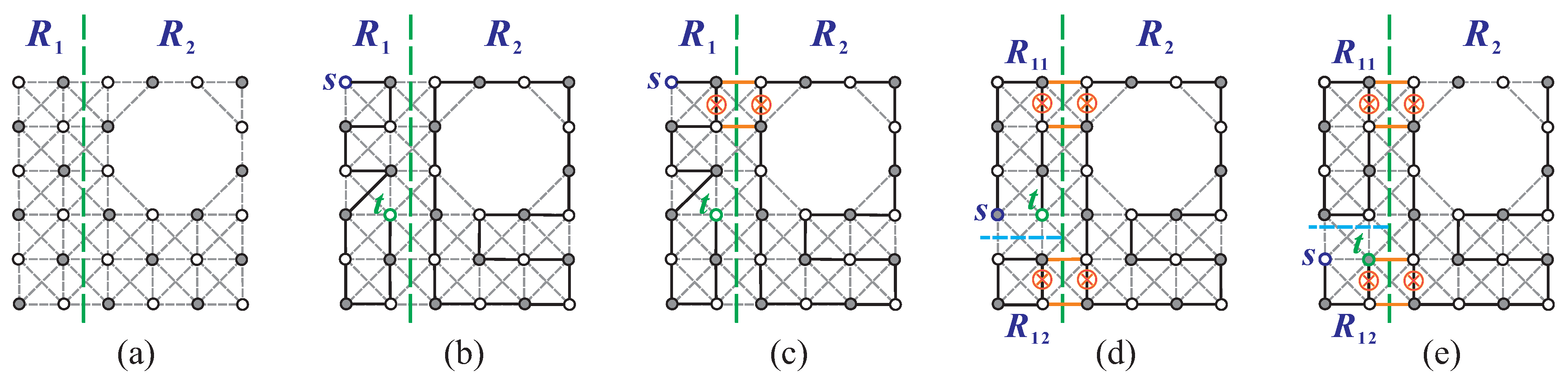
(F4)

$m=3$, $a=m-k=2$, and either of the following: $c=1$, and $\{s,t\}=\left\{\right(1,1),(2,2\left)\right\}$ or $\left\{\right(1,2),(2,1\left)\right\}$; or $d=1$, and $\{s,t\}=\left\{\right(1,n),(2,n-1\left)\right\}$ or $\left\{\right(1,n-1),(2,n\left)\right\}$ (see Figure 7d).

(F5)

$n=3$, $k=c=d=1$, and one the following:

 (1) $a⩾2$, $s_x=t_x=m-1$, and $|s_y-t_y|=2$ (see Figure 7e);

 (2) $a=2$, $s_x=1$, $t_x=2$, and $|s_y-t_y|=2$ (see Figure 7f);

 (3) $a>2$, $s_x<m-1$, and $t=(m-1,2)$ (see Figure 7g).

(F6)

$a=m-k=1$, and $s_y,t_y⩽c$ or $s_y,t_y>c+l$ (see Figure 7h).

Theorem 1

(See [19,20,21]). A Hamiltonian $(s,t)$-path exists in a rectangular, L-shaped, or C-shaped supergrid graph G with vertices s and t, if and only if $(G,s,t)$ does not satisfy conditions $\left(\mathrm{F}1\right)$–$\left(\mathrm{F}6\right)$.

The Hamiltonian $(s,t)$-path in $R(m,n)$ that was constructed in [19] is known as the canonical path. This path satisfies the property that it contains at least one boundary edge from each boundary.

Lemma 2

(See [19]). If $R(m,n)$ is a rectangular supergrid graph, such that $m,n⩾1$, and s and t are two distinct vertices of $R(m,n)$, and if condition $\left(\mathrm{F}1\right)$ is not satisfied, then there exists a canonical Hamiltonian $(s,t)$-path in $R(m,n)$, meaning that $HP\left(R\right(m,n),s,t)$ exists.

Assuming that $\left(R\right(m,n),s,t)$ does not satisfy condition (F1), we define three vertices $w=(1,1)$, $z=(2,1)$, and $f=(3,1)$ of $R(m,n)$ with $m⩾3$ and $n⩾2$. In [20], it was demonstrated that a Hamiltonian $(s,t)$-path Q exists in $R(m,n)$ with $(z,f)\in Q$ if the following condition (F7) is satisfied; otherwise, $(w,z)\in Q$.

(F7)

$n=2$ and $\{s,t\}\in \left\{\right\{w,z\},\{(1,1),(2,2)\},\{(2,1),(1,2)\left\}\right\}$, or $n⩾3$ and $\{s,t\}=\{w,z\}$.

The following lemma summarizes the previous results.

Lemma 3

(See [20]). Suppose that $R(m,n)$ is a rectangular supergrid graph with $m⩾3$ and $n⩾2$, and let s and t be two distinct vertices in $R(m,n)$. In addition, let $w=(1,1)$, $z=(2,1)$, and $f=(3,1)$. If $\left(R\right(m,n),s,t)$ does not satisfy condition $\left(\mathrm{F}1\right)$, then there exists a canonical Hamiltonian $(s,t)$-path Q in $R(m,n)$ such that $(z,f)\in Q$ if $\left(R\right(m,n),s,t)$ satisfies condition $\left(\mathrm{F}7\right)$, and $(w,z)\in Q$ otherwise.

In [21], we derived the following lemma for a three-rectangle $R(m,3)$.

Lemma 4

(See [21]). Let s and t be two distinct vertices of $R(m,3)$, and let $z_1=(m,1)$, $z_2=(m,2)$, and $z_3=(m,3)$ be three other vertices of $R(m,3)$. Let us suppose that $\{s,t\}\cap \{z_1,z_2,z_3\}=\varnothing$. Then, there exists a Hamiltonian $(s,t)$-path of $R(m,3)$ that contains both edges $e_{12}=(z_1,z_2)$ and $e_{23}=(z_2,z_3)$.

The Hamiltonicities of L-shaped and C-shaped supergrid graphs were verified in [20,21] as follows.

Theorem 2

(See [20,21]). Let us consider $L(m,n;k,l)$ (resp., $C(m,n;k,l;c,d)$) as an L-shaped (resp., C-shaped) supergrid graph. It contains a Hamiltonian cycle if and only if it does not satisfy condition $\left(\mathrm{F}8\right)$ (resp., $\left(\mathrm{F}9\right)$), which is defined as follows:

(F8)

There exists a vertex w in $L(m,n;k,l)$ such that $de{g}_{L(m,n;k,l)}\left(w\right)=1$.

(F9)

$a(=m-k)=1$, or there exists a vertex $w\in V\left(C\right(m,n;k,l;c,d\left)\right)$ satisfying $de{g}_{C(m,n;k,l;c,d)}\left(w\right)=1$.

The following propositions, which relate cycles, paths, and vertices, were presented in [7,18,19] and will be used in the proofs of our results.

Proposition 1

(See [7,18,19]). Let $C_1$ and $C_2$ be two cycles in a graph G that do not share any vertices; let $C_1$ and $P_1$ be a cycle and a path in G, such that $V\left(C_1\right)\cap V\left(P_1\right)=\varnothing$; and let x be a vertex in $G-V\left(C_1\right)$ or $G-V\left(P_1\right)$. The following statements hold true:

$\left(1\right)$ If there exist two edges $e_1\in C_1$ and $e_2\in C_2$ such that $e_1\approx e_2$, then $C_1$ and $C_2$ can be combined into a cycle of G (see Figure 8a).

Figure 8. Schematic diagrams of (a) Statement (1), (b) Statement (2), (c) Statement (3), and (d) Statement (4) of Proposition 1, where the cycles or paths are denoted by bold dashed lines, and the symbol ⊗ is used to signify the removal of an edge during their construction.

$\left(2\right)$ If there exist two edges $e_1\in C_1$ and $e_2\in P_1$ such that $e_1\approx e_2$, then $C_1$ and $P_1$ can be combined into a path of G (see Figure 8b).

$\left(3\right)$ If vertex x adjoins an edge $(u_1,v_1)$ of $C_1$ (or $P_1$), then $C_1$ (or $P_1$) and x can be combined into a cycle (or path) of G (see Figure 8c).

$\left(4\right)$ If there exists an edge $(u_1,v_1)\in C_1$ such that $u_1\sim start\left(P_1\right)$ and $v_1\sim end\left(P_1\right)$, then $C_1$ and $P_1$ can be combined into a cycle C of G (see Figure 8d).

We demonstrated in [19,20,21] that the problem of finding the longest $(s,t)$-path in $R(m,n)$, $L(m,n;k,l)$, and $C(m,n;k,l;c,d)$ can be resolved in linear time.

Theorem 3.

According to [19,20,21], an $(s,t)$-path of maximum length can be calculated in $O\left(mn\right)$ linear time for a rectangular supergrid graph $R(m,n)$ with $mn⩾2$, an L-shaped supergrid graph $L(m,n;k,l)$, or a C-shaped supergrid graph $C(m,n;k,l;c,d)$, given two distinct vertices s and t within the graph.

The focus of this paper is to examine the O-shaped supergrid graph denoted by $O(m,n;k,l;a,b,c,d)$, which has the structure illustrated in Figure 4c. Due to its symmetry, we limit our analysis to the following three cases, excluding the isomorphic ones:

• $a=b=c=d=1$;
• $a⩾2$ and $c=1$;
• $a,b,c,d⩾2$.

The above case that $a⩾2$ and $c=1$ can be further divided into four subcases: $b=d=1$, $b=1$ and $d⩾2$, $b⩾2$ and $d=1$, and $b,d⩾2$. These subcases are illustrated in Figure 9. Depending on the positions of s and t in $O(m,n;k,l;a,b,c,d)$, we can consider the following cases for the aforementioned three cases: $s_x,t_x⩽a$; $s_x⩽a$ and $t_x⩾a+1$; and $s_x,t_x⩾a+1$.

Figure 9. The subcases for $a⩾2$ and $c=1$: (a) $b=d=1$, (b) $b=1$ and $d⩾2$, (c) $b⩾2$ and $d=1$, and (d) $b,d⩾2$.

We first verify the Hamiltonicity of O-shaped supergrid graphs with the following theorem.

Theorem 4.

For any O-shaped supergrid graph $O(m,n;k,l;a,b,c,d)$, there exists a Hamiltonian cycle contained within it.

Proof. 

To obtain two disjoint supergrid subgraphs $R_1=R(a,n)$ and $R_2=C(m-a,n;$$k,l;c,d)$ from $O(m,n;k,l;a,b,c,d)$, we first make one vertical separation, as shown in Figure 10a. Let $p=(a,1)$ and $q=(a,n)$ be two vertices of $R_1$, and let $r_1=(a+1,1)$ and $r_2=(a+1,n)$ be two vertices of $R_2$, as depicted in Figure 10b. Note that $p\sim r_1$ and $q\sim r_2$. Since $(R_1,p,q)$ does not satisfy condition (F1), $(R_1,p,q)$ contains a Hamiltonian $(p,q)$-path $P_1$ according to Lemma 2. Similarly, $(R_2,r_2,r_1)$ contains a Hamiltonian $(r_2,r_1)$-path $P_2$ according to Theorem 1, as it does not satisfy conditions (F1)–(F2) and (F4)–(F6). Then, $P=P_1\Rightarrow P_2$ forms a Hamiltonian $(p,r_1)$-path of $O(m,n;k,l;a,b,c,d)$. Since $start\left(P\right)\sim end\left(P\right)$, P is a Hamiltonian cycle of $O(m,n;k,l;a,b,c,d)$. The constructed Hamiltonian cycle is depicted in Figure 10b.    □

Figure 10. (a) One vertical separation on $O(m,n;k,l;a,b,c,d)$ to obtain $R_1$ and $R_2$, and (b) the constructed Hamiltonian cycle of $O(m,n;k,l;a,b,c,d)$, with solid bold lines indicating the cycle.

We can see from the above construction that if $a=1$, then the constructed Hamiltonian cycle $HC$ of $O(m,n;k,l;$$a,b,c,d)$ satisfies $H{C}_{|R_1}$ being a flat face.

3. Forbidden Conditions for Hamiltonian Connectivity in O-Shaped Supergrid Graphs

This section aims to identify all cases where O-shaped supergrid graphs do not contain a Hamiltonian $(s,t)$-path. Although there are no cut vertices in these graphs, there are vertex cuts. Therefore, we have a forbidden condition, referred to as condition (F1), for the non-existence of $HP\left(O\right(m,n;k,l;a,b,c,d),s,t)$ (see Figure 11a,b).

Figure 11. $HP\left(O\right(m,n;k,l;a,b,c,d),s,t)$ does not exist when (a,b) $\{s,t\}$ is a vertex cut; (c,d) $a=b=c=d=1$; and (e) $c=1$, $a,b,d⩾2$, and $k⩾5$.

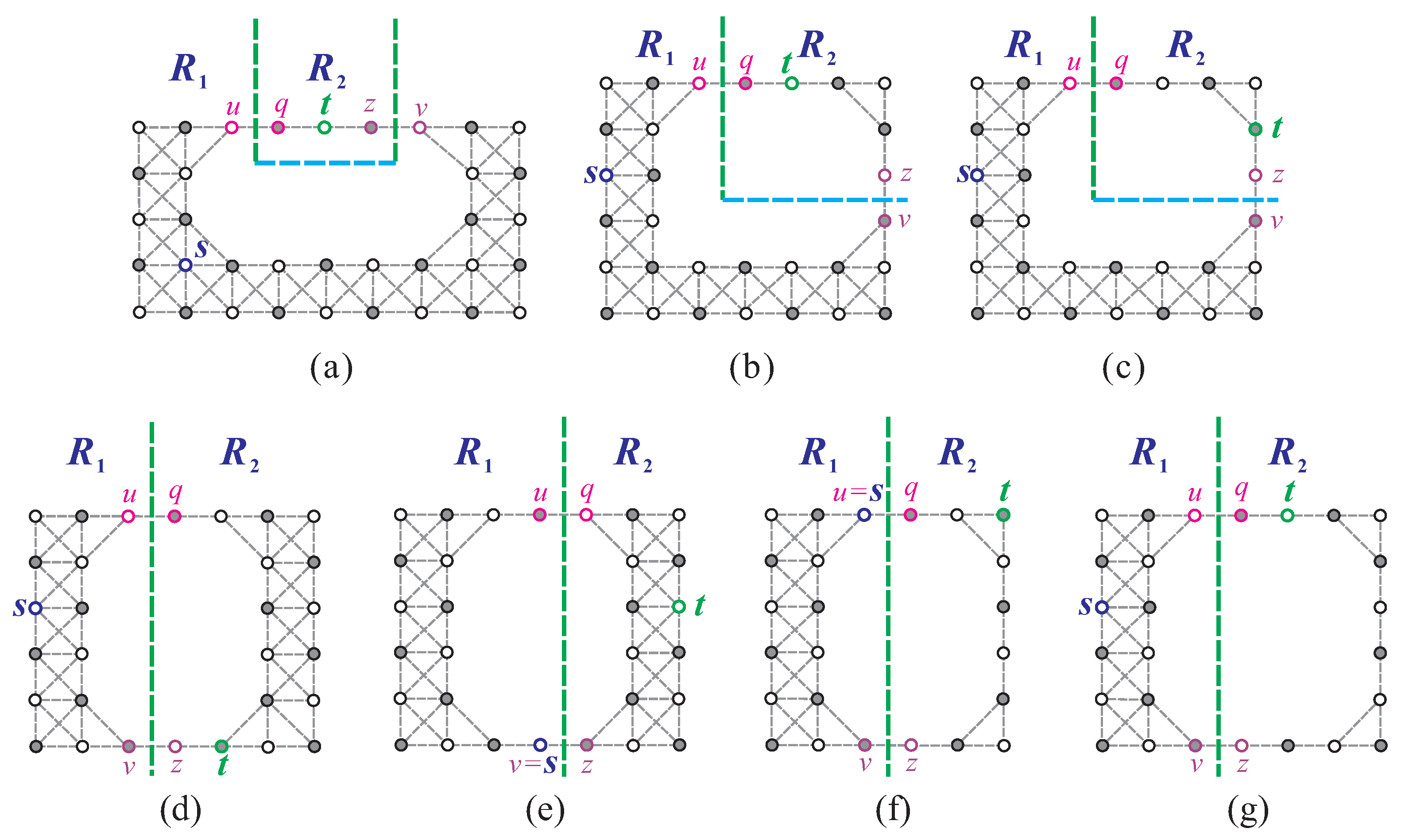
In the following, we explore the other forbidden conditions for the non-existence of a Hamiltonian $(s,t)$-path in O-shaped supergrid graphs. We examine the sizes of parameters a, b, c, and d, and list the forbidden conditions as follows.

(F10)

When $a=b=c=d=1$ and $s\nsim t$, $\{s,t\}$ is not a vertex cut, and one of the following cases occurs:

(1) $s\in \left\{\right(1,1),(1,n\left)\right\}$, $s_x\ne t_x$, and $s_y\ne t_y$ (see Figure 11c);

(2) $l⩾3$, $s\mathrm{or}t\in \left\{\right(1,1),(1,n\left)\right\}$, $s_x=t_x$, and $|s_y-t_y|>2$ (see Figure 11d).

(F11)

When $c=1$, $a,b,d⩾2$, $k⩾5$, and $s\nsim t$, $\{s,t\}$ is not a vertex cut, and $a+3⩽s_x\left(\mathrm{or}{t}_x\right)⩽a+k-2$ (see Figure 11e).

(F12)

$c=d=1$, $a,b⩾2$, $k⩾3$, and one of the following cases occurs:

(1) $s_x⩽a$ and $t_x⩾a+3$ (see Figure 12a);

Figure 12. For O-shaped supergrid graphs with $a⩾2$ and $c=1$, the forbidden conditions for the existence of a Hamiltonian $(s,t)$-path are as follows: (a) when $d=1$, $b⩾2$, $s_x⩽a$, and $t_x⩾a+3$; (b) when $d=1$, $b⩾2$, $a+1⩽s_x⩽a+k-2$, and $t_x⩾a+k+1$; and (c,d) when $b=1$, $s_x,t_x⩾a+1$, $t=(m,1)$, $k⩾3$, and $s_x⩽m-3$.

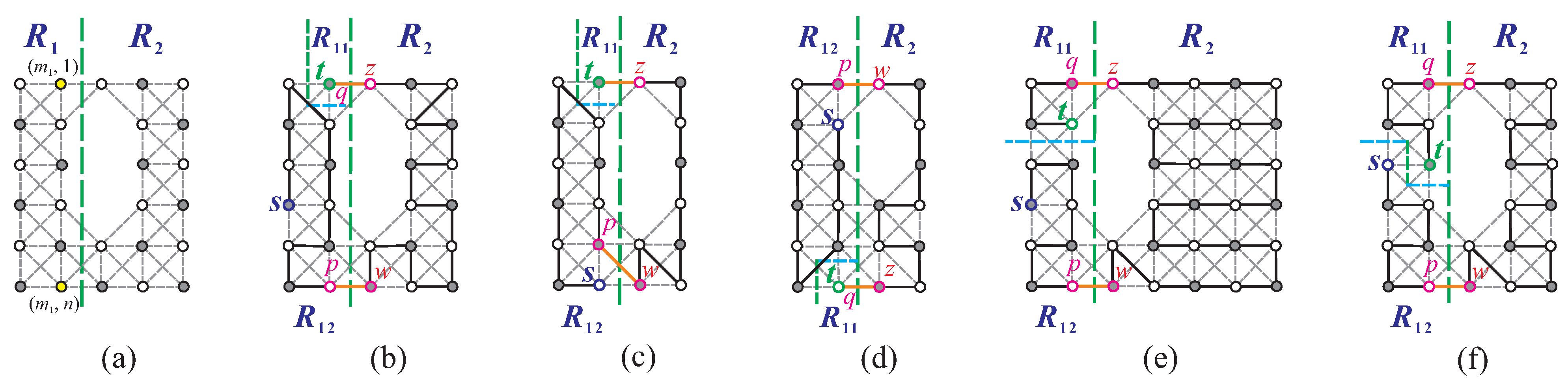
(2) $a+1⩽s_x⩽a+k-2$ and $t_x⩾a+k+1$ (see Figure 12b).

(F13)

$b=c=1$, $a⩾2$, $s\nsim t$, and one of the following cases occurs:

(1) $s_x,t_x⩾a+1$; $t=(m,1)$; $d=1$, or $d⩾2$ and $s_y,t_y⩽c+l$; and one of the following occurs:

   (1.1) $k⩾3$, $s_y=1$, and $s_x⩽m-3$ (see Figure 12c,d);

   (1.2) $s_y=n$ and $s_x⩽m-1$ (see Figure 13a);

Figure 13. O-shaped supergrid graphs with $a⩾2$ and $c=b=1$, in which there is no Hamiltonian $(s,t)$-path, where (a) case (1.2) of condition (F13) is satisfied, (b,c) case (1.3) of condition (F13) is satisfied, (d–f) case (2) of condition (F13) is satisfied, and (g,h) case (3) of condition (F13) is satisfied.

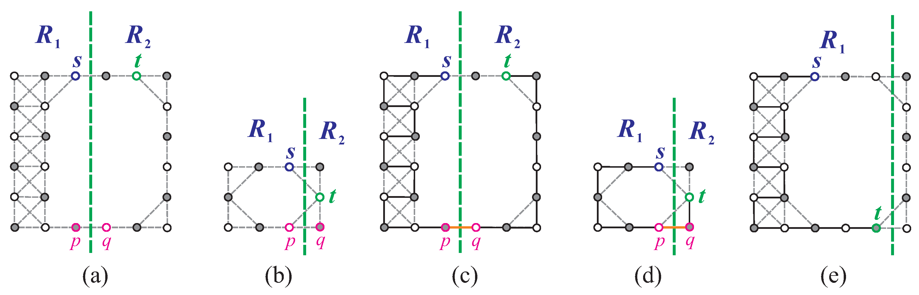
   (1.3) $l⩾3$, $s_x=t_x$, and $s_y⩾4$ (see Figure 13b,c);

(2) $d⩾2$; $t_x⩾a+1$; $t_y⩽c+l$; $s_x⩽a$, or $s_x⩾a+1$ and $s_y⩾c+l+1$; and one of the following occurs:

   (2.1) $k⩾3$, $t_y=1$, and $a+3⩽t_x⩽m-1$ (see Figure 13d);

   (2.2) $l⩾3$, $t_x=m$, and $2⩽t_y⩽l-1$ (see Figure 13e);

   (2.3) $k,l⩾3$ and $t=(m,1)$ (see Figure 13f);

(3) $d=1$; $s_x⩽a$; $t_x⩾a+1$; and $2⩽t_y⩽c+l$, or $k⩾3$ and $t_x⩾a+3$ (see Figure 13g,h).

The following lemma presents the necessary condition for the existence of a Hamiltonian $(s,t)$-path in O-shaped supergrid graph $O(m,n;k,l;a,b,c,d)$.

Lemma 5.

If $HP\left(O\right(m,n;k,l;a,b,c,d),s,t)$ exists, then $\left(O\right(m,n;k,l;a,b,c,d),s,t)$ must not satisfy conditions $\left(\mathrm{F}1\right)$ and $\left(\mathrm{F}10\right)$–$\left(\mathrm{F}13\right)$.

Proof. 

If $\left(O\right(m,n;k,l;a,b,c,d),s,t)$ satisfies any of conditions (F1) or (F10)–(F13), we can show that $HP\left(O\right(m,n;k,l;a,b,c,d),s,t)$ does not exist as follows: For condition (F1), the lemma clearly holds true, as shown in Figure 11a,b. For conditions (F10)–(F13), we can refer to Figure 11c–e, Figure 12, and Figure 13. Let v and u be two vertices depicted in these figures. It is clear that no Hamiltonian $(s,t)$-path in $O(m,n;k,l;a,b,c,d)$ can contain both vertices u and v.    □

All possible cases for the forbidden conditions for the existence of a Hamiltonian $(s,t)$-path in $O(m,n;k,l;a,b,c,d)$ are considered in this section. In the next section, we prove that if $\left(O\right(m,n;k,l;a,b,c,d),s,t)$ does not satisfy conditions (F1) and (F10)–(F13), then $O(m,n;k,l;a,b,c,d)$ contains a Hamiltonian $(s,t)$-path.

4. The Hamiltonian Connectivity of $\mathbf{O}$-Shaped Supergrid Graphs

This section aims to demonstrate the existence of a Hamiltonian $(s,t)$-path in $O(m,n;$$k,l;a,b,c,d)$ when $\left(O\right(m,n;k,l;a,b,c,d),s,t)$ does not satisfy conditions (F1) and (F10)–(F13). The following three lemmas consider the following three cases individually: $s_x,t_x⩽a$; $s_x⩽a$ and $t_x⩾a+1$; and $s_x,t_x⩾a+1$.

Lemma 6.

Let us assume that $O(m,n;k,l;a,b,c,d)$ is an O-shaped supergrid and that s and t are two distinct vertices in the graph. If $s_x,t_x⩽a$ and $\left(O\right(m,n;k,l;a,b,c,d),s,t)$ does not satisfy conditions $\left(\mathrm{F}1\right)$ and $\left(\mathrm{F}10\right)$, then it follows that $O(m,n;k,l;a,b,c,d)$ has a Hamiltonian $(s,t)$-path.

Proof. 

Due to symmetry, we only need to examine three cases: $a=b=c=d=1$; $a⩾2$ and $c=1$; and $a,b,c,d⩾2$. The cases that are isomorphic, as shown in Section 2, are not considered. Then, there are the following three cases.

Case 1: $a=b=c=d=1$. We first make a vertical separation on $O(m,n;k,l;a,b,c,d)$ to obtain two disjoint supergrid subgraphs $R_1=R(m_1,n)$ and $R_2=C(m-m_1,n;k,l;c,d)$, where $m_1=a$ (see Figure 14a). Then, we consider $s\sim t$, or $s\nsim t$ together with either $l⩽2$, or $l⩾3$ and either $s_y,t_y⩽3$ or $s_y,t_y⩾n-2$. Let the following hold: $s\nsim t$; $l⩾3$; and either $s,t\notin \left\{\right(1,1),(1,n\left)\right\}$, or s or $t\in \left\{\right(1,1),(1,n\left)\right\}$ and $|s_y-t_y|>2$. Then, $\left(O\right(m,n;k,l;a,b,c,d),s,t)$ satisfies condition (F1) or (F10). Without loss of generality, we assume that $t_y<s_y$, and for the case $s\nsim t$, we assume that $t=(1,1)$. We partition $R_1$ horizontally into two subgraphs $R_{11}$ and $R_{12}$, where $R_{11}=R(m_1,n_1)$ and $R_{12}=R(m_1,n-n_1)$, and $n_1=t_y$ if $s\sim t$; otherwise, $n_1=t_y+1$ (see Figure 14b,c). Let $q\in V\left(R_{11}\right)$, $p\in V\left(R_{12}\right)$, and $w,z\in V\left(R_2\right)$ such that $p\sim w$, $q\sim z$, $z=(m_1+1,1)$, $w=(m_1+1,n)$, $p=(m_1,n)$, and $q=(m_1,1)$ if $s\sim t$; otherwise, $q=(m_1,2)$. We consider $(R_2,w,z)$. Since $z_x=w_x=m_1+1=a+1$, $z_y=1$, and $w_y=n$, it is clear that $(R_2,w,z)$ does not satisfy conditions (F1)–(F2) and (F4)–(F6). We then consider $(R_{11},q,t)$ and $(R_{12},s,p)$. If either of these subgraphs satisfies condition (F1), then $\left(O\right(m,n;k,l;a,b,c,d),s,t)$ satisfies condition (F10), which is a contradiction. Therefore, neither $(R_{11},q,t)$ nor $(R_{12},s,p)$ satisfies condition (F1). As $(R_{12},s,p)$, $(R_{11},q,t)$, and $(R_2,w,z)$ fail to satisfy conditions (F1)–(F2) and (F4)–(F6), Theorem 1 implies the existence of Hamiltonian paths $P_1$, $P_2$, and $P_3$ in $R_{12}$, $R_2$, and $R_{11}$, respectively, with endpoints $(s,p)$, $(w,z)$, and $(q,t)$ (refer to Figure 14d). Concatenating these paths as $P=P_1\Rightarrow P_2\Rightarrow P_3$ results in a Hamiltonian $(s,t)$-path in $O(m,n;k,l;a,b,c,d)$, as shown in Figure 14e.

Figure 14. (a) A vertical separation on $O(m,n;k,l;a,b,c,d)$ is performed with the constraints that $s_x,t_x⩽a$, and $a=b=c=d=1$; (b,c) a horizontal separation is performed on $R_1$, where (b) assumes that s and t are adjacent and (c) assumes that s and t are non-adjacent; (d) Hamiltonian paths are constructed for $R_{11}$, $R_{12}$, and $R_2$; and (e) a Hamiltonian $(s,t)$-path is constructed in $O(m,n;k,l;a,b,c,d)$, with bold lines representing the constructed path.

Case 2: $a⩾2$ and $c=1$. We can divide this into two subcases based on the size of a:

Case 2.1: $a=2$. For this subcase, we begin by conducting a vertical separation on $O(m,n;k,l;a,b,c,d)$. This results in two separate supergrid subgraphs, $R_1=R(m_1,n)$ and $R_2=C(m-m_1,n;k,l;c,d)$, where $m_1=a$ (refer to Figure 15a). Depending on whether or not $s,t\in \{(m_1,1),(m_1,n)\}$, we consider the following subcases.

Figure 15. (a) A vertical separation on $O(m,n;k,l;a,b,c,d)$, where $s_x,t_x⩽a$, $a=2$, and $c=1$, is performed to obtain $R_1$ and $R_2$. (b–d,f) Vertical and horizontal separations on $R_1$ are performed. (e) A horizontal separation on $R_1$ is performed. Note that bold lines represent the constructed Hamiltonian path.

Case 2.1.1: s or $t\in \{(m_1,1),(m_1,n)\}$. We can assume, without loss of generality, that $t\in \{(m_1,1),(m_1,n)\}$. Then, $t=(m_1,1)$ or $t=(m_1,n)$ as the following two subcases.

Case 2.1.1.1: $t=(m_1,1)$. In this subcase, we first perform both vertical and horizontal separations on $R_1$, which results in two separated supergrid subgraphs, $R_{11}$ and $R_{12}$, with $R_{11}=R(1,t_y)$ and $R_{12}=L(m_1,n;1,t_y)$ (refer to Figure 15b,c). We then choose $q\in V\left(R_{11}\right)$, $p\in V\left(R_{12}\right)$, and $w,z\in V\left(R_2\right)$ such that $p\sim w$, $q\sim z$, $z=(m_1+1,1)$, $w=(m_1+1,n)$, $q=(m_1,1)=t$, and $p=(m_1,n)$ if $s\ne (m_1,n)$; otherwise, $p=(m_1,n-1)$. We then consider $(R_2,w,z)$ and $(R_{12},s,p)$ and show that they do not satisfy certain conditions necessary for the existence of a Hamiltonian $(s,t)$-path of $O(m,n;k,l;a,b,c,d)$. Specifically, $(R_2,w,z)$ violates conditions (F1)–(F2) and (F4)–(F6), since $z_x=w_x=m_1+1=a+1$, $z_y=1$, and $w_y=n$. On the other hand, $(R_{12},s,p)$ violates conditions (F1), (F2), and (F3), due to the relationship between s and p. Despite these complications, we can construct a Hamiltonian $(s,t)$-path of $O(m,n;k,l;a,b,c,d)$ by following an approach similar to that in Case 1. Figure 15b,c depict the Hamiltonian $(s,t)$-paths constructed in this subcase.

Case 2.1.1.2: $t=(m_1,n)$. In the case of $d=1$, we can construct a Hamiltonian $(s,t)$-path of $O(m,n;k,l;a,b,c,d)$ using symmetry, similarly to Case 2.1.1.1. Specifically, we set $R_{11}=R(1,1)$, $R_{12}=L(m_1,n;1,1)$, $q=(m_1,n)$, $p=(m_1,1)$, $w=(m_1+1,1)$, and $z=(m_1+1,n)$ (refer to Figure 15d). In the case of $d⩾2$, we perform vertical and horizontal separations on $R_1$ to obtain two disjoint supergrid subgraphs, $R_{11}$ and $R_{12}$, where $R_{11}=R(1,1)$ and $R_{12}=L(n,m_1;1,1)$ (see Figure 15d). We then choose $q\in V\left(R_{11}\right)$, $p\in V\left(R_{12}\right)$, and $w,z\in V\left(R_2\right)$ such that $p\sim w$, $q\sim z$, $z=(m_1+1,n)$, $w=(m_1+1,1)$, $q=(m_1,n)=t$, and $p=(m_1,1)$ if $s\ne (m_1,1)$; otherwise, $p=(m_1,2)$. We can then construct a Hamiltonian $(s,t)$-path of $O(m,n;k,l;a,b,c,d)$ using an approach similar to that in Case 1. An example of the Hamiltonian $(s,t)$-path constructed in this subcase is shown in Figure 15d.

Case 2.1.2: $s,t\notin \{(m_1,1),(m_1,n)\}$. Assuming $t_y⩽s_y$ without loss of generality, there are two cases to consider. First, let us consider $s_y\ne t_y$. In this case, a Hamiltonian $(s,t)$-path of $O(m,n;k,l;a,b,c,d)$ can be constructed similarly to Case 1, where $n_1=t_y$ (see Figure 15e). Next, let us consider $s_y=t_y$. Then, a Hamiltonian $(s,t)$-path of $O(m,n;k,l;a,b,c,d)$ can be constructed similarly to Case 2.1.1.1, where $R_{12}=L(m_1,n-n_1+1;1,1)$, $R_{11}=L(m_1,n_1;1,1)$, and $n_1=s_y$ (see Figure 15f). Figure 15e,f depict the Hamiltonian $(s,t)$-paths of $O(m,n;k,l;a,b,c,d)$ constructed in this subcase.

Case 2.2: $a⩾3$. To obtain two separated supergrid subgraphs $R_1=R(m_1,n)$ and $R_2=O(m-m_1,n;k,l;1,b,c,d)$, we perform a vertical separation on $O(m,n;k,l;a,b,c,d)$. The value of $m_1$ is determined as $a-1$, as shown in Figure 16a. The resulting subcases depend on the locations of s and t and can be categorized as the following three subcases.

Figure 16. (a) A vertical separation on $O(m,n;k,l;a,b,c,d)$, where $s_x,t_x⩽a$ and $a⩾3$; (b) a Hamiltonian $(s,t)$-path in $R_1$ and a Hamiltonian cycle in $R_2$; (c) a Hamiltonian $(s,t)$-path in $O(m,n;k,l;a,b,c,d)$, where $\{s,t\}$ is not a vertex cut of $R_{11}$; (d,e) horizontal separation on $R_1$ and Hamiltonian $(s,t)$-paths of $O(m,n;k,l;a,b,c,d)$, where $\{s,t\}$ is a vertex cut of $R_{11}$ and where in (b–e), s and t are in $R_1$, the constructed Hamiltonian $(s,t)$-path is indicated by bold lines, and ⊗ denotes the destruction of an edge during the construction of the Hamiltonian path.

Case 2.2.1: $s,t\in R_1$. Based on the value of $m_1$ and the relationship between $s_y$ and $t_y$, we can divide it into the following two subcases.

Case 2.2.1.1: Either $m_1⩾3$, or $m_1=2$ and one of the following: $s_y\ne t_y$, $s_y=t_y=1$, or $s_y=t_y=n$. In this subcase, $\{s,t\}$ is not a vertex cut of $R_1$ (refer to Figure 16b). We consider $(R_1,s,t)$ and check that it does not easily satisfy condition (F1). Therefore, according to Lemmas 3–4, there exists a Hamiltonian $(s,t)$-path $P_1$ in $R_1$ in which one edge $e_1$ faces $R_2$. Applying Theorem 4, $R_2$ contains a Hamiltonian cycle $H{C}_2$ such that one flat face faces $R_1$. Then, there exist two edges $e_1\in P_1$ and $e_2\in H{C}_2$ such that $e_1\approx e_2$ (as shown in Figure 16b). According to Statement (2) of Proposition 1, $P_1$ and $H{C}_2$ can be combined into a Hamiltonian $(s,t)$-path of $O(m,n;k,l;a,b,c,d)$. The construction of such a Hamiltonian path is depicted in Figure 16c.

Case 2.2.1.2: $m_1=2$ and $2⩽s_y=t_y⩽n-1$. In this subcase, $\{s,t\}$ is a vertex cut of $R_1$. We then separate $R_1$ horizontally into two disjoint supergrid subgraphs $R_{11}=R(m_1,n_1)$ and $R_{12}=R(m_1,n-n_1)$, where $n_1=s_y$ if $s_y\ne n-1$, and $n_1=s_y-1$ if $s_y=n-1$ (see Figure 16d,e). If $n_1=s_y$, then s and t belong to $R_{11}$; otherwise, they belong to $R_{12}$. Without loss of generality, let us assume that s and t are both in $R_{11}$. Since $s_y=t_y=n_1$, $(R_{11},s,t)$ does not satisfy condition (F1). By Lemmas 3 and 4, $R_{11}$ contains a Hamiltonian $(s,t)$-path $P_{11}$ in which one edge $e_{11}$ is facing $R_2$. By Lemma 1 and Theorem 4, $R_{12}$ and $R_2$ each contain a Hamiltonian cycle, $H{C}_{12}$ and $H{C}_2$, respectively. Hence, there exist four edges, i.e., $e_1$, $e_2\in H{C}_2$, $e_{11}\in P_{11}$, and $e_{12}\in H{C}_{12}$, such that $e_1\approx e_{11}$ and $e_2\approx e_{12}$, as illustrated in Figure 16d. By Statements (1) and (2) of Proposition 1, $P_{11}$, $H{C}_{12}$, and $H{C}_2$ can be combined into a Hamiltonian $(s,t)$-path of $O(m,n;k,l;a,b,c,d)$. The construction of such a Hamiltonian path is depicted in Figure 16d. For the case where s and t belong to $R_{12}$, a Hamiltonian $(s,t)$-path of $O(m,n;k,l;a,b,c,d)$ can be constructed in the same way, as shown in Figure 16e.

Case 2.2.2: $s,t\in R_2$. Since $s_x$ and $t_x$ are both less than or equal to a, we know that $s_x=t_x=a$ (refer to Figure 16a and Figure 17a). Without loss of generality, let $t_y<s_y$. We perform a vertical separation and a horizontal separation on $R_2$ to create three disjoint supergrid subgraphs $R_{21}=R(1,t_y)$, $R_{22}=R(1,n-t_y)$, and $R_{23}=C(m-m_1-1,n;k,l;c,d)$. Let $R_{\mathrm{a}}=R_1\cup R_{22}$. Then, $R_{\mathrm{a}}=L(a,n;1,t_y)$ (see Figure 17a). A Hamiltonian $(s,t)$-path of $O(m,n;k,l;a,b,c,d)$ can be constructed similarly to Case 2.1.1.1, where $p\in V\left(R_{\mathrm{a}}\right)$, $q\in V\left(R_{21}\right)$, and $w,z\in V\left(R_{23}\right)$ (see Figure 17a–c).

Figure 17. A Hamiltonian $(s,t)$-path of $O(m,n;k,l;a,b,c,d)$, where $a⩾3$ and $c=1$, for (a–c) $s,t\in R_2$; and (d) $s\in R_1$ and $t\in R_2$.

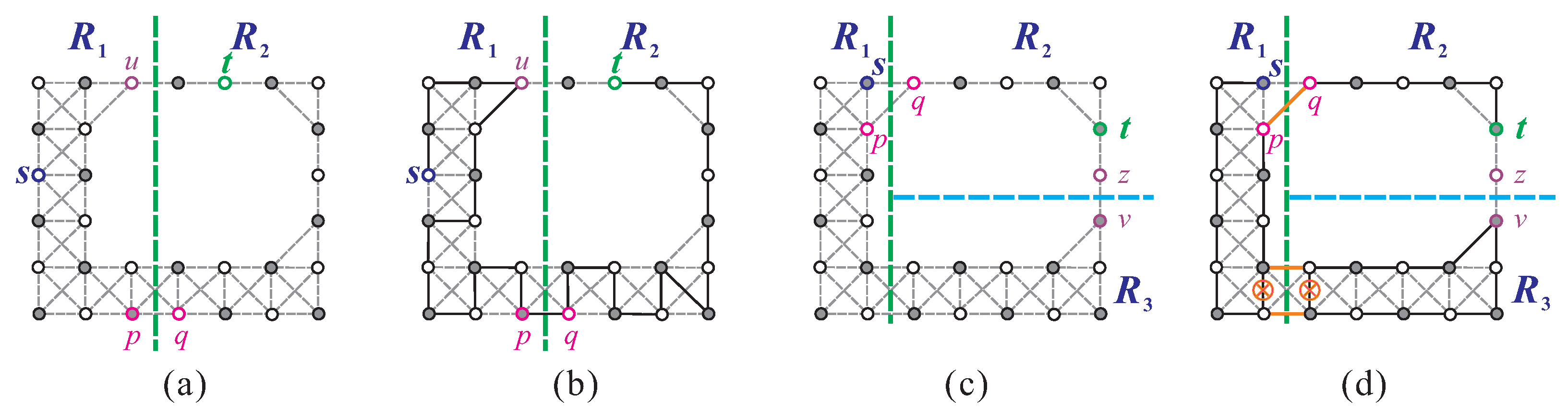
Case 2.2.3: $s\in R_1$ and $t\in R_2$. A Hamiltonian $(s,t)$-path of $O(m,n;k,l;a,b,c,d)$ can be constructed similarly to Case 2.2.2. Refer to Figure 17d for the construction of the path.

Case 3: $a,b,c,d⩾2$. To construct a Hamiltonian $(s,t)$-path of $O(m,n;k,l;a,b,c,d)$ when $a=2$, we can use the same approach as in Case 2.1. Similarly, for $a⩾3$, we can construct a Hamiltonian $(s,t)$-path of $O(m,n;k,l;a,b,c,d)$ using the same method as in Case 2.2.    □

Lemma 7.

Let us assume that $O(m,n;k,l;a,b,c,d)$ is an O-shaped supergrid and that s and t are two distinct vertices in the graph. If $s_x⩽a$, $t_x⩾a+1$, and $\left(O\right(m,n;k,l;a,b,c,d),s,t)$ does not satisfy conditions $\left(\mathrm{F}1\right)$ and $\left(\mathrm{F}10\right)$–$\left(\mathrm{F}13\right)$, then there exists a Hamiltonian $(s,t)$-path in $O(m,n;k,l;a,b,c,d)$.

Proof. 

Let us consider that $a=b=c=d=1$. In this case, $t_y=s_y$; $s\in \left\{\right(1,1),(1,n\left)\right\}$; and either $t_x⩽a+2$, or $k=2$ and $t\in \left\{\right(m,1),(m,n\left)\right\}$. Let the following hold: $k⩾3$; $t_x⩾a+3$; and either $s\in \left\{\right(1,1),(1,n\left)\right\}$ and $t_y\ne s_y$, or $s\notin \left\{\right(1,1),(1,n\left)\right\}$. Then, $\left(O\right(m,n;k,l;a,b,c,d),s,t)$ satisfies condition (F1) or (F10). So, $s_y=t_y=1$ or $s_y=t_y=n$, and it can be considered equivalent to Case 1 in Lemma 6. Thus, we assume that $a⩾2$ for the following cases. Additionally, for the case where $b=c=d=1$, we can assume without loss of generality that $s_y,t_y⩽c+l$. We now consider the following cases.

Case 1: $c=1$. In this case, $a⩾2$ and $c=1$. There are four subcases, each with different sizes of b, c, and d (refer to Figure 9). Depending on the placement of t, we examine the following subcases.

Case 1.1: $a+1⩽t_x⩽a+k$ and $t_y=1$. In this subcase, either $t_x⩽a+2$, or $b,d⩾2$ and $t_x⩾a+k-1$. Let the following hold: $b=1$ or $d=1$, $k⩾3$, and $t_x⩾a+3$; or $b,d⩾2$, $k⩾5$, and $a+3⩽t_x⩽a+k-2$. Then, $\left(O\right(m,n;k,l;a,b,c,d),s,t)$ satisfies (F11)–(F13). Note that the former ($b=1$ or $d=1$, $k⩾3$, and $t_x⩾a+3$) satisfy condition (F12) or (F13), and the latter ($b,d⩾2$, $k⩾5$, and $a+3⩽t_x⩽a+k-2$) satisfy condition (F11). Next, we can consider the subsequent subcases.

Case 1.1.1: $t_x=a+1$. First, we make a vertical separation on $O(m,n;k,l;a,b,c,d)$ and obtain two separated supergrid subgraphs: $R_1=R(m_1,n)$ and $R_2=C(m-m_1,n;k,l;$$c,d)$, where $m_1=a$ (refer to Figure 18a,b). We select $p\in V\left(R_1\right)$ and $q\in V\left(R_2\right)$ such that $p\sim q$, $q=(m_1+1,n)$, and $p=(m_1,n)$ if $s\ne (m_1,n)$; otherwise, $p=(m_1,n-1)$. Next, we consider $(R_2,q,t)$. As $t_y=1$ and $q_y=n$, it is evident that $(R_2,q,t)$ does not satisfy conditions (F1), (F2), and (F4)–(F6). We also examine $(R_1,s,p)$, where condition (F1) holds if $m_1=2$ and $s_y=p_y=n-1$. However, this contradicts the fact that $p=(m_1,n)$ when $s\ne (m_1,n)$. Therefore, $(R_1,s,p)$ does not satisfy condition (F1). Because $(R_1,s,p)$ and $(R_2,q,t)$ fail to satisfy conditions (F1), (F2), and (F4)–(F6), according to Theorem 1, there must exist a Hamiltonian $(s,p)$-path $P_1$ and a Hamiltonian $(q,t)$-path $P_2$ of $R_1$ and $R_2$, respectively (as shown in Figure 18c). Finally, $P=P_1\Rightarrow P_2$ yields a Hamiltonian $(s,t)$-path of $O(m,n;k,l;a,b,c,d)$, which is depicted in Figure 18d.

Figure 18. (a,b) A vertical separation on $O(m,n;k,l;a,b,c,d)$ for $a⩾2$, $c=1$, and $t=(a+1,1)$; (c) a Hamiltonian $(s,p)$-path in $R_1$ and a Hamiltonian $(q,t)$-path in $R_2$ for (a); (d) a Hamiltonian $(s,t)$-path in $O(m,n;k,l;a,b,c,d)$ for (a); and (e) a vertical separation on $O(m,n;k,l;a,b,c,d)$ and a Hamiltonian $(s,t)$-path in $O(m,n;k,l;a,b,c,d)$ for $a⩾2$, $c=1$, and $t=(a+2,1)$, where bold lines indicate the constructed Hamiltonian path.

Case 1.1.2: $t_x=a+2$. In this subcase, $k⩾2$. A Hamiltonian $(s,t)$-path of $O(m,n;k,l;$$a,b,c,d)$ can be constructed, following a method similar to that in Case 1.1.1, where we set $R_1=C(m_1,n;1,l;c,d)$ and $R_2=C(m-m_1,n;k-1,l;c,d)$, and set $m_1=a+1$ (refer to Figure 18e). The resulting Hamiltonian $(s,t)$-path of $O(m,n;k,l;a,b,c,d)$ is also shown in Figure 18e.

Case 1.1.3: $b,d⩾2$ and $t_x⩾a+k-1$. In this subcase, we have $a+k⩾t_x⩾a+k-1$. Therefore, either $t=(a+k,1)$, or $t=(a+k-1,1)$. Then, we have the following two subcases.

Case 1.1.3.1: $t=(a+k,1)$. In this subcase, we have that $k⩾3$. We can construct a Hamiltonian $(s,t)$-path for $O(m,n;k,l;a,b,c,d)$ by making two vertical separations and one horizontal separation on $O(m,n;k,l;a,b,c,d)$ resulting in two disjoint subgraphs $R_1=C(n,m;l+c,k;a,b)$ and $R_2=R(k,c)$, as shown in Figure 19a. We then select vertices $p\in V\left(R_1\right)$ and $q\in V\left(R_2\right)$ such that $p\sim q$, $q=(a+1,1)$ and $p=(a,1)$ if $s\ne (a,1)$; otherwise, $p=(a,2)$. Next, we consider $(R_1,s,p)$. Since $a,b,d⩾2$, we only need to show that $(R_1,s,p)$ fails to satisfy condition (F1). If $s_y=p_y=2$, then condition (F1) holds, but it contradicts $p=(a,1)$ when $s\ne (a,1)$. We then consider $(R_2,q,t)$. Since $q=(a+1,1)$ and $t=(a+k,1)$, it is clear that $(R_2,q,t)$ does not satisfy condition (F1). Similarly to Case 1.1.1, we construct a Hamiltonian $(s,t)$-path of $O(m,n;k,l;a,b,c,d)$. Figure 19a shows such a constructed Hamiltonian $(s,t)$-path.

Figure 19. (a) Two vertical separations and one horizontal separation on $O(m,n;k,l;a,b,c,d)$ for $a,b,d⩾2$, $c=1$, and $t=(a+k,1)$; (b) a vertical separation on $O(m,n;k,l;a,b,c,d)$ for $a,b,d⩾2$, $c=1$, and $t=(a+k-1,1)$; (c) a Hamiltonian $(s,t)$-path in $R_1$ and a Hamiltonian cycle in $R_2$ for (b); and (d) a Hamiltonian $(s,t)$-path in $O(m,n;k,l;a,b,c,d)$ for (b), where bold lines represent the constructed Hamiltonian path and ⊗ indicates the destruction of an edge while constructing such a Hamiltonian $(s,t)$-path.

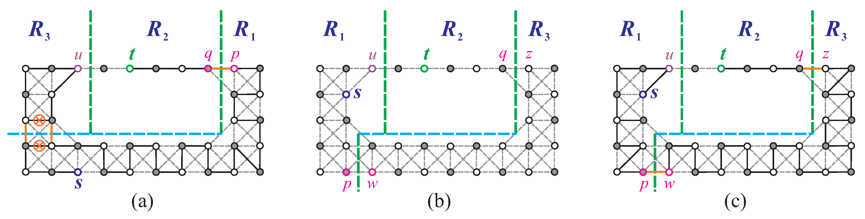
Case 1.1.3.2: $t=(a+k-1,1)$. In this subcase, we have $k⩾4$. We then perform a vertical separation on $O(m,n;k,l;a,b,c,d)$ to obtain two supergrid subgraphs $R_1=C(t_x,n;t_x-a,l;c,d)$ and $R_2=C(m-t_x,n;1,l;c,d)$ that are disjoint (refer to Figure 19b). We consider $(R_1,s,t)$ and note that since $a,d⩾2$, $t=(a+k-1,1)$, and $s_x⩽a$, it does not satisfy conditions (F1), (F2), and (F4)–(F6). Thus, according to Theorem 1, $R_1$ has a Hamiltonian $(s,t)$-path. We can construct a Hamiltonian $(s,t)$-path $P_1$ of $R_1$ using the algorithm in [21], and we can ensure that one edge $e_1$ of $P_1$ faces $R_2$. Using Theorem 2, $R_2$ contains a Hamiltonian cycle $H{C}_2$ that can be constructed so that one flat face of $H{C}_2$ faces $R_2$ (refer to Figure 19c). Thus, there are two edges $e_1\in P_1$ and $e_2\in H{C}_2$ such that $e_1\approx e_2$ (see Figure 19c). Using Statement (2) of Proposition 1, $P_1$ and $H{C}_2$ can be combined into a Hamiltonian $(s,t)$-path of $O(m,n;k,l;a,b,c,d)$. Figure 19d shows the construction of such a Hamiltonian path.

Case 1.2: $b=1$ and $t_y⩽c+l$. In this subcase, one of the following applies: $k⩽2$ or $l⩽2$, and $t=(m,1)$; or $d⩾2$ and $t_y⩾c+l-1$. If either $l⩾3$ and $2⩽t_y⩽c+l-2$, or $l,k⩾3$ and $t=(m,1)$, then $\left(O\right(m,n;k,l;a,b,c,d),s,t)$ satisfies condition (F13). According to the position of t, we consider the following three subcases.

Case 1.2.1: $t=(m,1)$. In this subcase, $k⩽2$ or $l⩽2$. We can divide this subcase into the following two subcases.

Case 1.2.1.1: $k⩽2$. We can construct a Hamiltonian $(s,t)$-path of $O(m,n;k,l;a,b,c,d)$ using an approach similar to that in Case 1.1.1. When $k=1$, we consider $R_1=R(m_1,n)$, $R_2=C(m-m_1,n;k,l;c,d)$, and $m_1=a$ (see Figure 20a). When $k=2$, we consider $R_1=C(a+1,n;1,l;c,d)$ and $R_2=C(m-a-1,n;1,l;c,d)$ (see Figure 20b). The Hamiltonian $(s,t)$-paths of $O(m,n;k,l;a,b,c,d)$ constructed using these cases are also depicted in Figure 20a,b.

Figure 20. (a,b) A vertical separation on $O(m,n;k,l;a,b,c,d)$ for $a⩾2$, $b=c=1$, $t=(m,1)$, and $k⩽2$; (c,d) vertical and horizontal separations on $O(m,n;k,l;a,b,c,d)$ for $a⩾2$, $b=c=1$, $t=(m,1)$, $k⩾3$, and $l⩽2$; (e) a Hamiltonian $(s,t)$-path in $R_1\cup R_2$ and a Hamiltonian cycle in $R_3$ for (c); and (f) a Hamiltonian $(s,t)$-path in $O(m,n;k,l;a,b,c,d)$ for (c).

Case 1.2.1.2: $k⩾3$ and $l⩽2$. To obtain three disjoint supergrid subgraphs $R_1=R(a,n)$, $R_2=L(m-a,n_1;k,n_1-c)$, and $R_3=R(m-a,d)$ if $l=1$ (otherwise, $R_3=L(m-a,n-n_1;k,l-n_1+c)$), where $n_1=t_y+1=2$ (see Figure 20c,d), we perform vertical and horizontal separations on $O(m,n;k,l;a,b,c,d)$. Then, we select $p\in V\left(R_1\right)$ and $q\in V\left(R_2\right)$, such that $p\sim q$, $q=(a+1,1)$ and $p=(a,1)$ if $s\ne (a,1)$; otherwise, $p=(a,2)$. We consider $(R_1,s,p)$ first. If $a=2$ and $s_y=p_y=2$, then condition (F1) is satisfied, which is a contradiction, since $p=(a,1)$ when $s\ne (a,1)$. Next, we consider $(R_2,q,t)$. Since $b=c=1$, $q=(a+1,1)$, and $t=(m,1)$, it is easy to check that $(R_2,q,t)$ does not satisfy conditions (F1), (F2), and (F3). Therefore, using Theorem 1, there exists a Hamiltonian $(s,p)$-path $P_1$ of $R_1$ and a Hamiltonian $(q,t)$-path $P_2$ of $R_2$. We note that $P_1$ is a canonical Hamiltonian path of $R_1$. Then, we obtain a Hamiltonian $(s,t)$-path of $R_1\cup R_2$ by combining $P_1$ and $P_2$, which is depicted in Figure 20e. Using Lemma 1, $R_3$ contains a canonical Hamiltonian cycle $H{C}_3$. We can place one flat face of $H{C}_3$ to face $R_1$. Then, we can find two edges $e_1\in P$ and $e_3\in H{C}_3$ such that $e_1\approx e_3$ (see Figure 20f). Using Statement (2) of Proposition 1, we can combine P and $H{C}_3$ into a Hamiltonian $(s,t)$-path of $O(m,n;k,l;a,b,c,d)$. The construction of such a Hamiltonian path is shown in Figure 20f.

Case 1.2.2: $t=(m,c+l)$. To construct a Hamiltonian $(s,t)$-path of $O(m,n;k,l;a,b,c,d)$, we follow an approach similar to that in Case 1.1.3.1, where two disjoint supergrid subgraphs $R_1=L(m,n;k+b,c+l)$ and $R_2=L(k+b,c+l;k,l)$ are as shown in Figure 21a,b.

Figure 21. (a–c) Vertical and horizontal separations on $O(m,n;k,l;a,b,c,d)$ for $a⩾2$, $b=c=1$, and $t=(m,c+l)$ or $t=(m,c+l-1)$; (d,e) a vertical separation on $O(m,n;k,l;a,b,c,d)$ for $a,d⩾2$ and $c=1$; and (f) a vertical separation on $O(m,n;k,l;a,b,c,d)$ for $a⩾2$, $c=1$, $s_y=t_y=1$, and $a+1⩽s_x,t_x⩽a+k$.

Case 1.2.3: $t=(m,c+l-1)$. In this subcase, $l⩾2$. A Hamiltonian $(s,t)$-path of $O(m,n;k,l;a,b,c,d)$ can be constructed similarly to Case 1.2.1.2. Here, let $n_1=t_y$ (as shown in Figure 21c).

Case 1.3: $d⩾2$ and one of the following: $b⩾2$, and either $t_y⩾2$, or $t_y=1$ and $t_x>a+k$; or $b=1$ and $t_y⩾c+l+1$. A Hamiltonian $(s,t)$-path of $O(m,n;k,l;a,b,c,d)$ can be constructed in a way similar to that in Case 1.1.1. We set q to be $(m_1+1,1)$, and if $s\ne (m_1,1)$, then $p=(m_1,1)$; otherwise, $p=(m_1,2)$ (refer to Figure 21d,e). Note that $d,b⩾2$; $q=(m_1+1,1)$; and either $t_x>a+k$, or $t_x⩽a+k$ and $t_y>c+l$. Therefore, it is easy to verify that $(R_2,q,t)$ does not satisfy conditions (F1), (F2), and (F4)–(F6).

Case 2: $a,b,c,d⩾2$. A Hamiltonian $(s,t)$-path of $O(m,n;k,l;a,b,c,d)$ can be constructed, similarly to Case 1.1.1, depicted in Figure 18c,d, where $m_1=a$ and where p and q are chosen as follows:

$$\left\{\begin{array}{cc}p=(m_1,n)\mathrm{and}q=(m_1+1,n),\hfill & \mathrm{if}s\ne (m_1,n)\mathrm{and}t\ne (m_1+1,n);\hfill \\ p=(m_1,1)\mathrm{and}q=(m_1+1,1),\hfill & \mathrm{if}s=(m_1,n)\mathrm{and}t=(m_1+1,n);\hfill \\ p=(m_1,n)\mathrm{and}q=(m_1+1,n-1),\hfill & \mathrm{if}s\ne (m_1,n)\mathrm{and}t=(m_1+1,n);\hfill \\ p=(m_1,n-1)\mathrm{and}q=(m_1+1,n),\hfill & \mathrm{otherwise}.\hfill \end{array}\right.$$

Let us consider $(R_2,q,t)$. As $b,c,$ and d are greater than or equal to 2, and $q_x=m_1+1$ and $t_x⩾m_1+1$, it is obvious that $(R_2,q,t)$ does not satisfy conditions (F1), (F2), and (F4)–(F6). Now, let us consider $(R_1,s,p)$. Condition (F1) holds only if $s_y=p_y=n-1$ or $s_y=p_y=2$. However, this contradicts $p=(m_1,n)$ when $s\ne (m_1,n)$ or $p=(m_1,1)$ when $s\ne (m_1,1)$. Therefore, $(R_1,s,p)$ does not satisfy condition (F1).

We have considered any case for constructing a Hamiltonian $(s,t)$-path of $O(m,n;k,l;$$a,b,c,d)$, where $s_x⩽a$ and $t_x⩾a+1$. Thus, this lemma holds true.    □

Lemma 8.

Let us assume that $O(m,n;k,l;a,b,c,d)$ is an O-shaped supergrid and that s and t are two distinct vertices in the graph. If $s_x,t_x⩾a+1$ and $\left(O\right(m,n;k,l;a,b,c,d),s,t)$ does not satisfy conditions $\left(\mathrm{F}1\right)$ and $\left(\mathrm{F}10\right)$–$\left(\mathrm{F}13\right)$, then there exists a Hamiltonian $(s,t)$-path in $O(m,n;k,l;a,b,c,d)$.

Proof. 

Using symmetry, we can only consider the cases of $a⩾2$ and $c=1$, and $a=b=c=d=1$ and $a,b,c,d⩾2$ (please refer to the discussion after Theorem 3). The cases of $a=b=c=d=1$ and $a,b,c,d⩾2$ are isomorphic to Lemmas 6 and 7. Thus, we assume that $a⩾2$ and $c=1$ in the following. If $c=d=1$ and $s_x,t_x⩽a+k$, then it must be the case that $s_y=t_y=1$ or $s_y=t_y=n$. If $s_y=1$ and $t_y=n$, then $\{s,t\}$ is a vertex cut of $O(m,n;k,l;a,b,c,d)$, which satisfies condition (F1). Therefore, without loss of generality, let us assume that $s_y=t_y=1$ when $c=d=1$ and $s_x,t_x⩽a+k$. We now consider the following three cases.

Case 1: One of the following cases holds:

        (1) $b⩾2$, and $(s_x,t_x>a+k)$ or $(s_x⩽a+k$ and $t_x>a+k)$;

        (2) $d⩾2$, and $s_y>c+l$ or $t_y>c+l$.

In these cases, let us assume that the vertex in the upper-right corner has coordinates $(1,1)$ if $b⩾2$, or in the down-right corner if $d⩾2$ in $O(m,n;k,l;a,b,c,d)$. Using the same arguments as in the proofs of Lemmas 6 and 7, we can construct a Hamiltonian $(s,t)$-path of $O(m,n;k,l;a,b,c,d)$ in these cases. It is worth noting that these cases are equivalent to the assumptions made in Lemmas 6 and 7.

Case 2: $s_y=t_y=1$ and $s_x,t_x⩽a+k$. If $s\nsim t$, then $\left(O\right(m,n;k,l;a,b,c,d),s,t)$ satisfies condition (F1). Thus, $s\sim t$. A Hamiltonian $(s,t)$-path of $O(m,n;k,l;a,b,c,d)$ can be constructed similarly to Case 1.1.1 of Lemma 7, where $R_1=C(m_1,n;m_1-a,l;c,d)$, $R_2=C(m-m_1,n;a+k-m_1,l;c,d)$, and $m_1=s_x$ (see Figure 21f).

Case 3: $b=c=1$; $d=1$, or $d⩾2$ and $s_y,t_y⩽c+l$; and $s_x=t_x=m$, or $s_x⩽m-1$ and $t_x=m$. A Hamiltonian $(s,t)$-path of $O(m,n;k,l;a,b,c,d)$ can be constructed in this case, assuming that the vertex in the upper-right corner has coordinates $(1,1)$. The construction is similar to that in Case 1 of Lemma 6, when $s_x=t_x=m$, and Lemma 7, when $s_x⩽a+k(=m-1)$ and $t_x=m$.    □

The Hamiltonian connectivity of O-shaped supergrid graphs is verified with the following theorem, which is based on Lemma 5 and Lemmas 6–8.

Theorem 5.

A Hamiltonian $(s,t)$-path exists in the O-shaped supergrid graph $O(m,n;k,l;a,b,c,$$d)$ with distinct vertices s and t, if and only if conditions $\left(\mathrm{F}1\right)$ and $\left(\mathrm{F}10\right)$–$\left(\mathrm{F}13\right)$ are not satisfied by $\left(O\right(m,n;k,l;a,b,c,d),s,t)$.

5. The Longest (s, t)-Path Algorithm

In Theorem 5, we know that if $\left(O\right(m,n;k,l;a,b,c,d),s,t)$ satisfies one of the conditions ((F1) and (F10)–(F13)), then $\left(O\right(m,n;k,l;a,b,c,d),s,t)$ contains no Hamiltonian $(s,t)$-path. So, in this section, for these cases, we first establish upper bounds on the lengths of the longest paths between s and t. We then demonstrate that these upper bounds are equivalent to the lengths of the longest $(s,t)$-paths in $O(m,n;k,l;a,b,c,d)$. It is worth noting that isomorphic cases are excluded, and we assume that $s_x⩽t_x$. The cases that we consider are limited to $a=b=c=d=1$, $a⩾2$, and $c=1$; and $a,b,c,d⩾2$ (see Section 2). In this context, we use $\widehat{L}(G,s,t)$ to denote the lengths of the longest paths between s and t, and $\widehat{U}(G,s,t)$ to represent the upper bound on the length of the longest paths between s and t, where G is a rectangular, L-shaped, C-shaped, or O-shaped supergrid graph. Note that the length of a path is defined as the number of vertices on the path. The following lemmas present these upper bounds.

Our initial focus is on the scenario where $\{s,t\}$ forms a vertex cut of $O(m,n;k,l;a,b,c,$$d)$. In this case, we determine the upper bound of the length of the longest $(s,t)$-path using the following lemma.

Lemma 9.

Let us assume that $c=1$ and that $\{s,t\}$ is a vertex cut of $O(m,n;k,l;a,b,c,d)$. The following conditions are satisfied:

$\left(\mathrm{O}1\right)$

If $k⩾3$ and $s_y=t_y=1$, then the length of any path between s and t cannot exceed $m\times n-k\times l-t_x+s_x+1$ (refer to Figure 22a).

Figure 22. The upper bound of the length of the longest $(s,t)$-path, where $\{s,t\}$ is a vertex cut, when (a) (O1) holds, (b) (O2) holds, and (c,d) (O3) holds. Note that a vertical separation in $O(m,n;k,l;a,b,c,d)$ is denoted by a bold dashed line.

$\left(\mathrm{O}2\right)$

If $b=1$, $a+1⩽s_x⩽a+k$, $s_y=1$, and $t_x=m$, then the length of any path between s and t cannot exceed $m\times n-k\times l-t_y-m+s_x+2$ (refer to Figure 22b).

$\left(\mathrm{O}3\right)$

If $d=1$, $a+1⩽s_x,t_x⩽a+k$, $s_y=1$, and $t_y=n$, then the length of any path between s and t cannot exceed $max\{\widehat{L}(R_1,s,t),\widehat{L}(R_2,s,t)\}$, where $R_1=C(t_x,n;t_x-a,l,c,d)$, $R_2=C(m-m_1,n;a+k-m_1,l,c,d)$, and $m_1=s_x-1$ (refer to Figure 22c,d).

Proof. 

Let us consider Figure 22a–d. When we remove s and t from $O(m,n;k,l;a,b,$$c,d)$, we obtain two separated components, $R_1$ and $R_2$. Therefore, any simple path between s and t can only pass through one of these components, implying that its length cannot exceed the size of the largest component. For condition (O1) (resp., condition (O2)), the length of any path between s and t is equal to $max\{t_x-s_x+1,m\times n-k\times l-t_x+s_x+1\}$ (resp., $max\{t_y+m-s_x,m\times n-k\times l-t_y-m+s_x+2\}$). Since $a\times n+b\times n+d\times k>t_x-s_x+1$ (resp., $a\times n+d\times (k+b)>t_y+m-s_x$), it is apparent that the length of any path between s and t cannot exceed $m\times n-k\times l-t_x+s_x+1$ (resp., $m\times n-k\times l-t_y-m+s_x+2$).    □

The next lemma provides an upper bound for the length of the longest $(s,t)$-path in $O(m,n;k,l;a,b,c,d)$, when $\{s,t\}$ is not a vertex cut and $c=1$, under the assumption that the graph satisfies conditions (F11)–(F13).

Lemma 10.

Let $\left(O\right(m,n;k,l;a,b,c,d),s,t)$ satisfy condition $\left(\mathrm{F}11\right)$, $\left(\mathrm{F}12\right)$, or $\left(\mathrm{F}13\right)$ (cases $\left(1.1\right)$, $\left(1.2\right)$, $\left(2\right)$, and $\left(3\right)$ of $\left(\mathrm{F}13\right)$). Then, the following implications hold true:

$\left(1\right)$

If $\left(O\right(m,n;k,l;a,b,c,d),s,t)$ satisfies condition $\left(\mathrm{F}11\right)$, then the length of any $(s,t)$-path cannot exceed $max\{m\times n-k\times l-t_x+u_x+1,m\times n-k\times l-v_x+t_x+1\}$, where $u=(a+1,1)$, $v=(a+k,1)$, $t_y=1$, and $a+3⩽t_x⩽a+k-2$ (refer to Figure 23a).

Figure 23. The upper bound of the length of the longest $(s,t)$-path in $O(m,n;k,l;a,b,c,d)$ for (a) condition (F11); (b) case (2.1) of condition (F13); (c) cases (2.2) and (2.3) of condition (F13); (d,e) condition (F11); and (f,g) cases (1.1), (1.2), and (3) of condition (F13), where the bold dash line indicates vertical or horizontal separation on $O(m,n;k,l;a,b,c,d)$.

$\left(2\right)$

If $\left(O\right(m,n;k,l;a,b,c,d),s,t)$ satisfies case (2.1) of condition $\left(\mathrm{F}13\right)$, then the length of any $(s,t)$-path cannot exceed $max\{m\times n-k\times l-t_x+u_x+1,m\times n-k\times l-z_y-m+t_x+1\}$, where $u=(a+1,1)$, $z=(m,c+l-1)$, $t_y=1$, and $a+3⩽t_x⩽m-1$ (refer to Figure 23b).

$\left(3\right)$

If $\left(O\right(m,n;k,l;a,b,c,d),s,t)$ satisfies case (2.2) or (2.3) of condition $\left(\mathrm{F}13\right)$, then the length of any $(s,t)$-path cannot exceed $max\{m\times n-k\times l-m+u_x-t_y+2,m\times n-k\times l-v_y+t_y+1\}$, where $u=(a+1,1)$, $v=(m,c+l)$, $t_x=m$, and $1⩽t_y⩽l-1$ (refer to Figure 23c).

$\left(4\right)$

If $\left(O\right(m,n;k,l;a,b,c,d),s,t)$ satisfies condition $\left(\mathrm{F}12\right)$, case (1.1) or (3) of $\left(\mathrm{F}13\right)$, then the length of any $(s,t)$-path cannot exceed $max\{\widehat{L}(R_1,s,u)+\widehat{L}(R_2,q,t),\widehat{L}(R_1,s,v)+\widehat{L}(R_2,z,t)\}$ (refer to Figure 23d,e and Figure 23f,g), where $u=(m_1,1)$, $q=(m_1+1,1)$, $v=(m_1,n)$, $z=(m_1+1,n)$, $R_1=C(m_1,n;m_1-a,l;c,d)$, and $R_2=C(m-m_1,n;a+k-m_1,l;c,d)$ if $k>1$ (otherwise, $R_2=R(b,n)$), and $m_1=a+1$ if $s_x⩽a$ (otherwise, $m_1=s_x$).

Proof. 

Let us examine Figure 23. It is evident that for the longest $(s,t)$-path P in $O(m,n;k,l;$$a,b,c,d)$, starting from s, P must traverse all or some vertices of $R_1$, exit $R_1$ via u or v, enter $R_2$ via q or z, and terminate at t. Therefore, the length of any path between s and t cannot exceed $max\{\widehat{L}(R_1,s,u)+\widehat{L}(R_2,q,t),\widehat{L}(R_1,s,v)+\widehat{L}(R_2,z,t)\}$.    □

We finally consider the remaining conditions for the case where $\{s,t\}$ is not a vertex cut of $O(m,n;k,l;a,b,c,d)$. Specifically, we consider condition (F10) and case (1.3) of condition (F13).

Lemma 11.

Let $a=c=1$ and $s=(1,1)$. If $\left(O\right(m,n;k,l;a,b,c,d),s,t)$ satisfies the following condition $\left(\mathrm{O}4\right)$, then the length of any $(s,t)$-path cannot exceed $max\{\widehat{L}(R_1,s,u)+\widehat{L}(R_2,q,t),$$\widehat{L}(R_1,s,v)+\widehat{L}(R_2,z,t)\}$ (see Figure 24a–c), where $R_1=C(n_1,m;1,k;a,b)$ and $R_2=C(n-n_1,m;l-1,k;a,b)$ if $l>1$; otherwise, $R_2=R(m,d)$, $n_1=1$, $u=(1,c+1)$, $q=(1,c+2)$, $v=(m,c+1)$, and $z=(m,c+2)$.

Figure 24. The upper bound of the length of the longest $(s,t)$-path in $O(m,n;k,l;a,b,c,d)$ for condition (O4), where (a,b) $d=1$, $t_y=n$, and $s_x\ne t_x$; and (c) $s_x=t_x$, $l⩾3$, and $t_y⩾4$.

Condition $\left(\mathrm{O}4\right)$ is defined below.

(O4)

One of the following cases holds:

(1)

$d=1$, $t_y=n$, and $s_x\ne t_x$ (case (1) of condition (F10));

(2)

$s_x=t_x$, $l⩾3$, and $t_y⩾4$ (case (2) of condition (F10) and case (1.3) of condition (F13)).

Proof. 

The proof follows an approach similar to that of Lemma 10 and can be visualized in Figure 24a–c.    □

Let us define condition (O0) as follows:

$\left(\mathrm{O}0\right)$

None of the conditions (F1), (F10), (F11), (F12), or (F13) are satisfied by $\left(O\right(m,n;k,l;$$a,b,c,d),s,t)$.

Checking whether any $\left(O\right(m,n;k,l;a,b,c,d),s,t)$ satisfies one of conditions (O0), (O1), (O2), (O3), (O4), (F11), (F12), and (F13) is a straightforward task. If $\left(O\right(m,n;k,l;$$a,b,c,d),s,t)$ satisfies (O0), then $\widehat{U}\left(O\right(m,n;k,l;$$a,b,c,d),s,t)=mn-kl$. Otherwise, $\widehat{U}(O$$(m,n;k,l;a,b,c,d),s,t)$ can be calculated using Lemmas 9–11. These calculations are summarized below, where $\left|G\right|=m\times n-k\times l$:

$\widehat{U}(O(m,n;k,l;a,b,c,d),s,t)=\left\{\begin{array}{cc}\left|G\right|-t_x+s_x+1,\hfill & \mathrm{if}\left(\mathrm{O}1\right)\mathrm{holds};\hfill \\ \left|G\right|-t_y-m+s_x+2,\hfill & \mathrm{if}\left(\mathrm{O}2\right)\mathrm{holds};\hfill \\ max\{\widehat{L}(R_1,s,t),\widehat{L}(R_2,s,t)\},\hfill & \mathrm{if}\left(\mathrm{O}3\right)\mathrm{holds};\hfill \\ max\left\{\right|G|-t_x+u_x+1,|G|-v_x+t_x+1\},\hfill & \mathrm{if}\left(\mathrm{F}11\right)\mathrm{holds};\hfill \\ max\left\{\right|G|-t_x+u_x+1,|G|-z_y-m+t_x+1\},\hfill & \mathrm{if}\mathrm{case}\left(2.1\right)\mathrm{of}\left(\mathrm{F}13\right)\mathrm{holds};\hfill \\ max\left\{\right|G|-m+u_x-t_y+2,|G|-v_y+t_y+1\},\hfill & \mathrm{if}\mathrm{case}\left(2.2\right)\mathrm{or}\left(2.3\right)\mathrm{of}\left(\mathrm{F}13\right)\mathrm{holds};\hfill \\ max\{\widehat{L}(R_1,s,u)+\widehat{L}(R_2,q,t),\widehat{L}(R_1,s,v)+\widehat{L}(R_2,z,t)\},\hfill & \mathrm{if}\left(\mathrm{O}4\right),\left(\mathrm{F}12\right),\mathrm{or}\left(\mathrm{F}13\right)\left(\mathrm{case}1.1\mathrm{or}3\right)\mathrm{holds};\hfill \\ mn-kl,\hfill & \mathrm{if}\left(\mathrm{O}0\right)\mathrm{holds}.\hfill \end{array}\right.$

Next, we demonstrate how to find the longest $(s,t)$-path for O-shaped supergrid graphs. It should be noted that if $\left(O\right(m,n;k,l;a,b,c,d),s,t)$ satisfies condition (O0), then according to Theorem 5, it contains a Hamiltonian $(s,t)$-path.

Lemma 12.

When $\left(O\right(m,n;k,l;a,bc,d),s,t)$ satisfies any of conditions $\left(\mathrm{O}1\right)$–$\left(\mathrm{O}4\right)$ and $\left(\mathrm{F}11\right)$–$\left(\mathrm{F}13\right)$, it follows that $\widehat{L}(O(m,n;k,l;a,b,c,d),s,t)=\widehat{U}(O(m,n;k,l;a,b,c,d),s,t)$.

Proof. 

To prove this lemma, we construct an $(s,t)$-path P with length equal to $\widehat{U}\left(O\right(m,n;k,l;$$a,b,c,d),s,t)$. We consider the following cases.

Case 1: Conditions (O1) and (O2) hold. Using Lemma 9, we obtain $\widehat{U}(O(m,n;k,l;a,b,c,d),s,t)=m\times n-k\times l-t_x+s_x+1$ and $\widehat{U}(O(m,n;k,l;a,b,c,d),s,t)=m\times n-k\times l-t_y-m+s_x+2$ for conditions (O1) and (O2), respectively. We consider Figure 22a,b and make a vertical separation on $O(m,n;k,l;a,b,c,d)$ to create two disjoint supergrid subgraphs $R_1=C(m_1,n;m_1-a,l;c,d)$, and either $R_2=C(m-m_1,n;a+k-m_1,l;c,d)$ if $s_x\ne m-1$ or $R_2=R(b,n)$ if $s_x=m-1$, where $m_1=s_x$ (see Figure 25a,b). We select a vertex $p\in V\left(R_1\right)$ and a vertex $q\in V\left(R_2\right)$ such that $p\sim q$, $p=(m_1,n)$, and $q=(m_1+1,n)$. We then construct the longest $(s,p)$-path $P_1$ in $R_1$ and the longest $(q,t)$-path $P_2$ in $R_2$ using the algorithms from [19,21]. Finally, we create an $(s,t)$-path $P=P_1\Rightarrow P_2$, which forms the longest $(s,t)$-path of $O(m,n;k,l;a,b,c,d)$. Figure 25c,d demonstrate the construction of such longest $(s,t)$-path. The length of the constructed longest $(s,t)$-path equals $\widehat{L}(R_1,s,p)+\widehat{L}(R_2,q,t)=m\times n-k\times l-t_x+s_x+1$ or $m\times n-k\times l-t_y-m+s_x+2$.

Figure 25. (a,b) Vertical separation on $O(m,n;k,l;a,b,c,d)$ for conditions (O1) and (O2) respectively; (c,d) the longest $(s,t)$-path in $O(m,n;k,l;a,b,c,d)$ for (a,b), respectively; and (e) the longest $(s,t)$-path in $O(m,n;k,l;a,b,c,d)$ for (O3), where bold lines indicate the constructed longest $(s,t)$-path.

Case 2: Condition (O3) holds. Using Lemma 9, we can express $\widehat{U}(O(m,n;k,l;a,b,c,d),s,t)$ as $max\{\widehat{L}(R_1,s,t),\widehat{L}(R_2,s,t)\}$, where $R_1$ and $R_2$ are two disjoint subgraphs of $O(m,n;k,l;a,b,c,d)$ (refer to Figure 22c,d). Since $R_1$ and $R_2$ are both C-shaped supergrid graphs, we can apply the algorithm from [21] to construct the longest path between s and t in either $R_1$ or $R_2$. The construction of such a path is shown in Figure 25e. The length of the constructed path is equal to $\widehat{L}(R_1,s,t)$ or $\widehat{L}(R_2,s,t)$, which in turn is equal to $\widehat{U}(O(m,n;k,l;a,b,c,d),s,t)$ by Lemma 9.

Case 3: Condition (F11) holds. Let us examine Figure 23a. According to Lemma 10, if $\left(O\right(m,n;k,l;a,b,c,d),s,t)$ satisfies condition (F11), then $\widehat{U}(O(m,n;k,l;a,b,c,d),s,t)=\ell$, where $\ell =max\{m\times n-k\times l-t_x+u_x+1,m\times n-k\times l-v_x+t_x+1\}$. There are two subcases to consider.

Case 3.1: $\ell =m\times n-k\times l-v_x+t_x+1$. We begin by making two vertical separations and one horizontal separation on $O(m,n;k,l;a,b,c,d)$ to obtain three disjoint supergrid subgraphs, $R_1=L(m,n;k+b,c+l)$, $R_2=R(k-1,c)$, and $R_3=L(b+1,c+l;1,l)$, as shown in Figure 26a. Let $p\in V\left(R_1\right)$ and $q\in V\left(R_2\right)$, such that $p\sim q$, $q=(a+1,1)$, and $p=(a,1)$ if $s\ne (a,1)$; otherwise, $p=(a,2)$. We consider $(R_1,s,p)$ and note that it does not satisfy conditions (F1)–(F3). Using the algorithms from [19,20], we can construct a Hamiltonian $(s,p)$-path $P_1$ in $R_1$ and the longest $(q,t)$-path $P_2$ in $R_2$. We can construct $P_1$ such that its one edge is placed to face $R_3$ using the algorithm from [20]. Then, $P_{12}=P_1\Rightarrow P_2$ forms the longest $(s,t)$-path of $R_1\cup R_2$, as depicted in Figure 26b. According to Theorem 2, $R_3$ contains a Hamiltonian cycle $H{C}_3$. Using the algorithm in [20], we can construct $H{C}_3$ such that its one flat face faces $R_1$. Then, there exist two edges, $e_1\in P_{12}$ and $e_3\in H{C}_3$, such that $e_1\approx e_3$ (see Figure 26c). Using Statement (2) of Proposition 1, we can combine $P_{12}$ and $H{C}_3$ into the longest $(s,t)$-path P of $O(m,n;k,l;a,b,c,d)$. The construction of such longest path is depicted in Figure 26c. The length of the constructed longest $(s,t)$-path is equal to $\widehat{L}(R_1,s,p)+\widehat{L}(R_2,q,t)+\left|V\left(R_3\right)\right|=m\times n-k\times l-v_x+t_x+1$.

Figure 26. (a) Two vertical separations and one horizontal separation on $O(m,n;k,l;a,b,c,d)$ for (F11), where $\ell =m\times n-k\times l-v_x+t_x+1$; (b) the longest $(s,t)$-path in $R_1\cup R_2$ and a Hamiltonian cycle of $R_3$; and (c) the longest $(s,t)$-path in $O(m,n;k,l;a,b,c,d)$ for (a), where bold lines indicate the constructed longest $(s,t)$-path and ⊗ represents the destruction of an edge while constructing such an $(s,t)$-path.

Case 3.2: $\ell =m\times n-k\times l-t_x+u_x+1$. Let us examine the following scenarios.

Case 3.2.1: $s_x>a$. Let $(1,1)$ be the coordinates of the vertex in the upper-right corner of $O(m,n;k,l;a,b,c,d)$. Then, we can construct the longest $(s,t)$-path of $O(m,n;k,l;a,b,c,d)$ in a way similar to that in Case 3.1 (as shown in Figure 27a).

Figure 27. (a) The longest $(s,t)$-path in $O(m,n;k,l;a,b,c,d)$ for condition (F11), where $\ell =m\times n-k\times l-t_x+u_x+1$ and $s_x>a$; (b) three vertical separations and one horizontal separation on $O(m,n;k,l;a,b,c,d)$ for (F11), where $\ell =m\times n-k\times l-t_x+u_x+1$ and $s_x⩽a$; and (c) the longest $(s,t)$-path in $O(m,n;k,l;a,b,c,d)$ for (b).

Case 3.2.2: $s_x⩽a$. We begin by partitioning $O(m,n;k,l;a,b,c,d)$ into three non-overlapping subgraphs, $R_1=L(a+1,n;1,n-c)$, $R_2=R(k-1,c)$, and $R_3=L(m-a,n;k,c+l)$, using three vertical separations and one horizontal separation (refer to Figure 27b). Let $p\in V\left(R_1\right)$, $q\in V\left(R_2\right)$, and $w,z\in V\left(R_3\right)$ such that $p\sim w$, $q\sim z$, $q=(a+k,1)$, $z=(a+k+1,1)$, $w=(a+1,n)$, and $p=(a,n)$ if $s\ne (a,n)$; otherwise, $p=(a,n-1)$. We observe that $(R_1,s,p)$ and $(R_3,w,z)$ do not satisfy conditions (F1)–(F3). To construct a Hamiltonian $(s,p)$-path $P_1$ and a Hamiltonian $(w,z)$-path $P_3$ of $R_1$ and $R_3$, respectively, we use the algorithm proposed in [20]. Using the algorithm proposed in [19], we construct the longest $(q,t)$-path $P_2$ in $R_2$. Finally, we concatenate $P_1$, $P_3$, and $P_2$ to obtain the longest $(s,t)$-path P of $O(m,n;k,l;a,b,c,d)$, i.e., $P=P_1\Rightarrow P_3\Rightarrow P_2$. The size of the constructed longest $(s,t)$-path is $\widehat{L}(R_1,s,p)+\widehat{L}(R_3,w,z)+\widehat{L}(R_2,q,t)=m\times n-k\times l-t_x-u_x+1$. We illustrate the construction of such longest $(s,t)$-path of $O(m,n;k,l;a,b,c,d)$ in Figure 27c.

Case 4: Case 2 of Condition (F13) holds. Let us consider Figure 23b,c. Based on Lemma 10, we have $\widehat{U}(O(m,n;k,l;a,b,c,d),s,t)=\ell$, where ℓ is the maximum of two values: ${\ell }_1=m\times n-k\times l-t_x+u_x+1$ and ${\ell }_2=m\times n-k\times l-z_y-m+t_x+1$ (or ${\ell }_1=m\times n-k\times l-u_x-t_y+2$ and ${\ell }_2=m\times n-k\times l-v_y+t_y+1$, depending on the subcase). We consider the following two subcases.

Case 4.1: $\ell =m\times n-k\times l-t_x+u_x+1$ (resp., $\ell =m\times n-k\times l-m+u_x-t_y+2)$. The longest $(s,t)$-path of $O(m,n;k,l;a,b,c,d)$ can be obtained in a way similar to that in Case 1, by making two vertical separations on $O(m,n;k,l;a,b,c,d)$ to obtain two disjoint supergrid subgraphs $R_1=C(m_1,n;m_1-a,l;c,d)$ and $R_2=C(m-m_1,n;a+k-m_1,l;c,d)$, where $m_1=a+1$, $q=(m_1+1,n)$ and $p=(m_1,n)$ (see Figure 28a). Using Lemma 10, the size of the constructed longest $(s,t)$-path is $\widehat{L}(R_1,s,p)+\widehat{L}(R_2,q,t)=m\times n-k\times l-t_x+u_x+1$ (resp., $m\times n-k\times l-m+u_x-t_y+2$). The construction of such longest $(s,t)$-path of $O(m,n;k,l;a,b,c,d)$ is depicted in Figure 28b.

Figure 28. (a) A vertical separation on $O(m,n;k,l;a,b,c,d)$ for case (2) of condition (F13), where $\ell =m\times n-k\times l-t_x+u_x+1$; (b) the longest $(s,t)$-path in $O(m,n;k,l;a,b,c,d)$ for (a); (c) a vertical separation and horizontal separations on $O(m,n;k,l;a,b,c,d)$ for case (2) of condition (F13), where $\ell =m\times n-k\times l-z_y-m+t_x+1$; and (d) the longest $(s,t)$-path in $O(m,n;k,l;a,b,c,d)$ for (c).

Case 4.2: $\ell =m\times n-k\times l-z_y-m+t_x+1$ (resp., $\ell =m\times n-k\times l-v_y+t_y+1)$. The longest $(s,t)$-path of $O(m,n;k,l;a,b,c,d)$ can be constructed in a way similar to that in Case 3.1. Let $R_1=R(m_1,n)$, $R_2=L(m-m_1,c+l-1;k,l-1)$, $R_3=L(m-m_1,d+1;k,1)$, $m_1=a$, $q=(m_1+1,1)$, and $p=(m_1,1)$ if $s\ne (m_1,1)$; otherwise, $p=(m_1,2)$ (see Figure 28c). The size of the constructed longest $(s,t)$-path is equal to $\widehat{L}(R_1,s,p)+\widehat{L}(R_2,q,t)+\left|V\left(R_3\right)\right|=m\times n-k\times l-z_y-m+t_x+1$ (resp., $m\times n-k\times l-v_y+t_y+1)$. The construction of such longest $(s,t)$-path of $O(m,n;k,l;a,b,c,d)$ is illustrated in Figure 28d.

Case 5: Condition (F13) (cases 1.1 and 3), (F12), or (O4) holds. Using Lemma 10 or 11, we can express $\widehat{U}(O(m,n;k,l;a,b,c,d),s,t)$ as $max\{\widehat{L}(R_1,s,u)+\widehat{L}(R_2,q,t),\widehat{L}(R_1,s,v)+\widehat{L}(R_2,z,t)\}$. To construct the longest $(s,t)$-path of $O(m,n;k,l;a,b,c,d)$, we consider Figure 23d–g and Figure 24. Since $R_1$ and $R_2$ are C-shaped supergrid graphs, we can use the algorithm proposed in [21] to construct the longest $(s,u)$-path $P_{11}$, the longest $(s,v)$-path $P_{12}$ in $R_1$, the longest $(q,t)$-path $P_{21}$, and the longest $(z,t)$-path $P_{22}$ in $R_2$. Then, we can form the longest $(s,t)$-path of $O(m,n;k,l;a,b,c,d)$ by concatenating $P_{11}$ and $P_{21}$, or $P_{12}$ and $P_{22}$.    □

Finally, we conclude with the following theorem.

Theorem 6.

Let $O(m,n;k,l;a,b,c,d)$ be an O-shaped supergrid graph with vertices s and t. Then, there exists a linear-time algorithm for finding the longest $(s,t)$-path of $O(m,n;k,l;a,b,c,d)$.

Proof. 

The algorithm presented in Algorithm 1 solves the problem in linear time by combining the results of Lemmas 9–12 and Theorem 5. Therefore, the theorem follows.    □

Algorithm 1: The longest $(s,t)$-path algorithm

Input: An O-shaped supergrid graph $O(m,n;k,l;a,b,c,d)$ and two distinct vertices s and t in it. Output: The longest $(s,t)$-path. if $s_x,t_x⩽a$ then output $HP\left(O\right(m,n;k,l;a,b,c,d),s,t)$ constructed from Lemma 6; // $\left(O\right(m,n;k,l;a,b,c,d),s,t)$ does not satisfy the forbidden conditions (F1) and (F10); if $s_x⩽a$ and $t_x⩾a+1$ then output $HP\left(O\right(m,n;k,l;a,b,c,d),s,t)$ constructed from Lemma 7; // $\left(O\right(m,n;k,l;a,b,c,d),s,t)$ does not satisfy the forbidden conditions (F1) and (F10)–(F13); if $s_x,t_x⩾a+1$ then output $HP\left(O\right(m,n;k,l;a,b,c,d),s,t)$ constructed from Lemma 8; // $\left(O\right(m,n;k,l;a,b,c,d),s,t)$ does not satisfy the forbidden conditions (F1) and (F10)–(F13); if $\left(O\right(m,n;k,l;a,b,c,d),s,t)$ satisfies one of the forbidden conditions (F1)and (F10)–(F13), then output the longest $(s,t)$-path based on Lemma 12.

6. Conclusions

We provide the necessary conditions for the existence of a Hamiltonian path in O-shaped supergrid graphs between any two given vertices. Moreover, we show that these necessary conditions are sufficient, by presenting a linear-time algorithm for computing the Hamiltonian path between any two vertices, except for five forbidden conditions. Hence, O-shaped supergrid graphs are Hamiltonian-connected, except in the case of the five forbidden conditions. Furthermore, we present a linear-time algorithm for computing the longest $(s,t)$-path of an O-shaped supergrid graph for any two given vertices s and t, provided that the forbidden conditions are satisfied. These algorithms can be regarded as the first attempts to solve the Hamiltonian and longest $(s,t)$-path problems for supergrid graphs with holes, where O-shaped supergrid graphs form a special class of supergrid graphs with holes. Although the Hamiltonian and longest $(s,t)$-path problems are NP-complete for general supergrid graphs, their complexities are still unknown for supergrid graphs with or without holes. We leave them as open problems for interested readers.

References

- Garey, M.R.; Johnson, D.S. Computers and Intractability: A Guide to the Theory of NP-Completeness; Freeman: San Francisco, CA, USA, 1979. [Google Scholar]
- Johnson, D.S. The NP-complete column: An ongoing guide. J. Algorithms 1985, 6, 434–451. [Google Scholar] [CrossRef]
- Bertossi, A.A.; Bonuccelli, M.A. Hamiltonian circuits in interval graph generalizations. Inform. Process. Lett. 1986, 23, 195–200. [Google Scholar] [CrossRef]
- Damaschke, P. The Hamiltonian circuit problem for circle graphs is NP-complete. Inform. Process. Lett. 1989, 32, 1–2. [Google Scholar] [CrossRef]
- Golumbic, M.C. Algorithmic Graph Theory and Perfect Graphs, 2nd ed.; Annals of Discrete Mathematics 57; Elsevier: Amsterdam, The Netherlands, 2004. [Google Scholar]
- Gordon, V.S.; Orlovich, Y.L.; Werner, F. Hamiltonian properties of triangular grid graphs. Discrete Math. 2008, 308, 6166–6188. [Google Scholar] [CrossRef]
- Hung, R.W.; Yao, C.C.; Chan, S.J. The Hamiltonian properties of supergrid graphs. Theor. Comput. Sci. 2015, 602, 132–148. [Google Scholar] [CrossRef]
- Krishnamoorthy, M.S. An NP-hard problem in bipartite graphs. SIGACT News 1976, 7, 26. [Google Scholar] [CrossRef]
- Itai, A.; Papadimitriou, C.H.; Szwarcfiter, J.L. Hamiltonian paths in grid graphs. SIAM J. Comput. 1982, 11, 676–686. [Google Scholar] [CrossRef]
- Bondy, J.A.; Murty, U.S.R. Graph Theory with Applications; Macmillan: London, UK; Elsevier: New York, NY, USA, 1976. [Google Scholar]
- Hung, R.W.; Keshavarz-Kohjerdi, F.; Tseng, Y.M.; Qiu, G.H. Finding longest (s, t)-paths of O-shaped supergrid graphs in linear time. In Proceedings of the 10th IEEE International Conference on Awareness Science and Technology 2019 (iCAST’2019), Morioka, Japan, 23–25 October 2019; pp. 252–259. [Google Scholar]
- Hung, R.W.; Keshavarz-Kohjerdi, F. The longest (s, t)-paths of O-shaped supergrid graphs. arXiv 2019, arXiv:1911.08558. [Google Scholar]
- Zamfirescu, C.; Zamfirescu, T. Hamiltonian properties of grid graphs. SIAM J. Discret. Math. 1992, 5, 564–570. [Google Scholar] [CrossRef]
- Chen, S.D.; Shen, H.; Topor, R. An efficient algorithm for constructing Hamiltonian paths in meshes. Parallel Comput. 2002, 28, 1293–1305. [Google Scholar] [CrossRef]
- Lenhart, W.; Umans, C. Hamiltonian cycles in solid grid graphs. In Proceedings of the 38th Annual Symposium on Foundations of Computer Science (FOCS’97), Miami Beach, FL, USA, 20–22 October 1997; pp. 496–505. [Google Scholar]
- Keshavarz-Kohjerdi, F.; Bagheri, A. Hamiltonian paths in L-shaped grid graphs. Theor. Comput. Sci. 2016, 621, 37–56. [Google Scholar] [CrossRef]
- Nishat, R.I.; Srinivasan, V.; Whitesides, S. 1-complex s, t Hamiltonian paths: Structure and reconfiguration in rectangular grids. J. Graph Algorithms Appl. 2023, 27, 281–327. [Google Scholar] [CrossRef]
- Hung, R.W. Hamiltonian cycles in linear-convex supergrid graphs. Discret. Appl. Math. 2016, 211, 99–112. [Google Scholar] [CrossRef]
- Hung, R.W.; Li, C.F.; Chen, J.S.; Su, Q.S. The Hamiltonian connectivity of rectangular supergrid graphs. Discret. Optim. 2017, 26, 41–65. [Google Scholar] [CrossRef]
- Keshavarz-Kohjerdi, F.; Hung, R.W. The Hamiltonicity, Hamiltonian connectivity, and longest (s, t)-path of L-shaped supergrid graphs. IAENG Int. J. Comput. Sci. 2020, 47, 378–391. [Google Scholar]
- Keshavarz-Kohjerdi, F.; Hung, R.W. Finding Hamiltonian and longest (s, t)-paths of C-shaped supergrid graphs in linear time. Algorithms 2022, 15, 61. [Google Scholar] [CrossRef]
Disclaimer/Publisher’s Note: The statements, opinions and data contained in all publications are solely those of the individual author(s) and contributor(s) and not of MDPI and/or the editor(s). MDPI and/or the editor(s) disclaim responsibility for any injury to people or property resulting from any ideas, methods, instructions or products referred to in the content. |
© 2023 by the authors. Licensee MDPI, Basel, Switzerland. This article is an open access article distributed under the terms and conditions of the Creative Commons Attribution (CC BY) license (https://creativecommons.org/licenses/by/4.0/).