Abstract
Face images in the logarithmic space can be considered as a sum of the texture component and lighting map component according to Lambert Reflection. However, it is still not easy to separate these two parts, because face contour boundaries and lighting change boundaries are difficult to distinguish. In order to enhance the separation quality of these to parts, this paper proposes an illumination standardization algorithm based on extreme L0 Gaussian difference regularization constraints, assuming that illumination is massively spread all over the image but illumination change boundaries are simple, regular, and sparse enough. The proposed algorithm uses an iterative L0 Gaussian difference smoothing method, which achieves a more accurate lighting map estimation by reserving the fewest boundaries. Thus, the texture component of the original image can be restored better by simply subtracting the lighting map estimated. The experiments in this paper are organized with two steps: the first step is to observe the quality of the original texture restoration, and the second step is to test the effectiveness of our algorithm for complex face classification tasks. We choose the facial expression classification in this step. The first step experimental results show that our proposed algorithm can effectively recover face image details from extremely dark or light regions. In the second step experiment, we use a CNN classifier to test the emotion classification accuracy, making a comparison of the proposed illumination removal algorithm and the state-of-the-art illumination removal algorithm as face image preprocessing methods. The experimental results show that our algorithm works best for facial expression classification at about 5 to 7 percent accuracy higher than other algorithms. Therefore, our algorithm is proven to provide effective lighting processing technical support for the complex face classification problems which require a high degree of preservation of facial texture. The contribution of this paper is, first, that this paper proposes an enhanced TV model with an L0 boundary constraint for illumination estimation. Second, the boundary response is formulated with the Gaussian difference, which strongly responds to illumination boundaries. Third, this paper emphasizes the necessity of reserving details for preprocessing face images.
MSC:
41K68
1. Introduction
Illumination variation is an unavoidable natural phenomenon in digital face images and videos. However, overexposure, backlight, dark light, and other extremely light environments will destroy the surface texture of the face image, especially the grayscale image. Face imaging under these environments will seriously affect the effectiveness of a series of related applications, i.e., face recognition [1], facial expression classification [2], facial muscle motor unit (AU) recognition, semantic classroom surveillance [3,4], etc. Therefore, the illumination removal problem of face images has been studied for years to alleviate the impact of extreme lighting conditions for classification and recognition. Among the illumination processing algorithms proposed in the literature, the LTV [5] and TVL1 [6] models are the most precise and promising for illumination separation in logarithmic face images. Both of these two models are based on the overall smoothness and large-scale assumption of the illumination component, always making it difficult to remove the edge produced by strong illumination variation, due to the lack of consideration for the complexity of the lighting conditions in face images, and this kind of edge produced by the illumination variability is very common in the face image. For example, face images shot under dark-light conditions are prone to partial exposure, making the exposure area different from the normal image by introducing strong bright and dark boundaries.While photographed under strong-light conditions, it is very easy to introduce obvious shadows to the face image, producing the light and dark boundary between the shadow area and the normal area. Since facial expression information is mainly conveyed by the main contours of the eyes, ears, mouth, and nose, it is required to include as few light and shade changes as possible in the facial expression’s sensitive detailed regions, so as not to affect the discriminative information of facial expressions. In our opinion, the most key point of illumination processing is to remove the bright and dark boundary and align the bright and dark regions without weakening or destroying the intrinsic contour of the face image. This is not achieved very well by most existing light processing methods, which still leaves a great margin to leverage the recognition performance of facial expressions. Thus, we proposed a new TV-based model which mostly considers the sparsity of the DoG (difference of Gaussian) to relieve the edge confusion problem between illumination parts and texture parts. The rest of the paper is organized as follows. In Section 2, the majority of the underlying theory illumination normalization techniques are briefly reviewed, and state-of-the-art algorithms are described. The novel Gaussian difference regularized model is presented in Section 3, and the solution of the smoothing part in the frequency domain and the solution of the regular part of this model are described in Section 4 and Section 5. The final algorithm summarized from our model is described in Section 6 with experimental evaluation in Section 7. The paper concludes with some final discussion in Section 8.
2. Related Work
The main purpose of this section is to classify and summarize the illumination processing methods proposed in the literature in recent years. Three basic principles or domains were extracted from the literature: the Lambert reflection criteria, Weber’s law, and the illumination separation in logarithmic space. We could say that almost all illumination processing algorithms, except deep-learning-based approaches [7,8,9], are designed upon one or more of these basics.
- The Lambert Reflection CriteriaLambert’s cosine law (Lambert’s cosine law) is a classic optical concept: it points out that the brightness of the diffuse reflection surface under detailed conditions is proportional to the ambient light intensity and is proportional to the cosine of the angle between the light direction vector and the normal vector of the diffuse reflection surface value:where is the rate of reflection with a certain material, L is the ambient light intensity, and is the angle between the light direction vector and the surface where the diffuse reflection occurs. Generally, the Lambert reflection occurs on material with a rough surface.
- Weber’s LawWeber’s law refers to a psychological phenomenon discovered by Ernst Weber, an experimental psychologist in the 19th century. It is pointed out that the animal’s sense of stimulus change is proportional to the intensity of the stimulus it receives:In the formula, I generally refers to the intensity of a certain sensory stimulus, is regarded as the change of sensory stimulus, and K is a constant. The Weberface [10,11] feature briefly combines Weber’s law and the Lambert Reflection surface, it eliminates illumination changes by constructing a gradient map of local perceptual intensity, and it obtains a gradient image with constant illumination:can be regarded as the human visual stimulation variation at pixel in the image, and uniquely corresponds to the position P in the real diffuse surface. Under the condition of Lambert diffuse reflection, , is the surrounding area of point P, which has same light reflection rate, and . Thus, . The Weberface [10,11] feature can be regarded as an illumination invariant feature that is only related to the light reflectance of the diffuse reflection sub-plane in the three-dimensional surface and will not affected by the intensity of light and the direction of light. The Weberface [10,11] algorithm eliminates the influence of illumination through the neighborhood properties of the diffuse surface, which can be regarded as a generalized gradient feature map. Although it has certain illumination invariance property, it can be proved by experiments that it has a positive significance for improving the accuracy of face recognition. However, due to the loss of real details of the image, such as adjacent points in the subtle slow reflection plane with the same light reflectivity, there is , so , and only using the Weberface feature map as the input of the expression recognition algorithm to distinguish the expression will cause the pattern recognition vector to be too sparse, thus affecting recognition accuracy. The gradientface [12] uses the face gradient directly as the illumination invariant, which was proposed earlier than Weberface. The success of this algorithm was also based also on Weber’s law.
- Illumination separation in logarithmic spaceIn the logarithmic space of the image, the frequency domain analysis method can be used to perform low-pass filtering on the logarithmic image to reduce the influence of light on the image. Take the logarithm on both sides of the Formula (1) at the pixel point :Thus, the logarithm of the whole image can be divided into two images, and . Obviously, under the premise of a given imaging surface, the imaging changes caused by the variation in illumination intensity and direction are mainly concentrated in , and can be considered the illumination invariant. From this clue, the researchers proposed methods to separate the illumination invariant features of the face in the logarithmic grayscale image from two perspectives: 1. illumination separation based on low-pass filtering, and 2. illumination separation based on the logarithmic grayscale image smoothing algorithm.
- Illumination separation based on high-pass filterHigh-pass filtering transforms the signal into the frequency domain, causes shrinkage, or removes the frequency coefficients in the low-frequency part and restores the signal from pruned frequency coefficients. It is widely used in electronic audio processing to block bass signals that could interfere or damage speakers. Considering the logarithmic grayscale image, can linearly separated into and , the component expressing illumination changes and always changing slowly when not reaching the shadow bound. It can be considered mainly concentrated in the low-frequency component in the frequency domain of . The Cos [13] algorithm uses the discrete cosine transform to convert the logarithmic grayscale image in the frequency domain, carefully removes the cosine response values that may contain the illumination component from the low-frequency cosine corresponding values, and then uses the inverse discrete cosine transform to obtain a large face image with the magnitude of the illumination effect removed. However, no matter how this algorithm selects the low-frequency cosine response value that needs to be eliminated, it will inevitably damage the image details while eliminating the illumination component and introduce waves in the final result.
- Illumination separation based on TV modelImage smoothing algorithms are generally used to denoise images that contain a lot of noise. After years of research, very satisfactory results have been achieved. At present, the image smoothing algorithm mainly focuses on noise reduction without damaging the edge of the object in the image. Therefore, the mature research results in this field are also used to separate the illumination component from the logarithmic grayscale image. Its processing method is just opposite of the idea based on high-pass filtering, that is, the overall design goal of the algorithm is to analyze the smooth illumination component , and the material inherent component is regarded as noise to be removed. Finally, the illumination component is removed from the image to obtain the intrinsic texture image with the illumination invariant property. Among the image smoothing algorithms, the TV [5] (total variance) model has attracted widespread attention from academia and industry due to its simplicity, appropriate model assumptions, and ease of acceleration using existing numerical analysis tools. The model generally assumes that images of the real world are all in the low variation space and proposes a simple equation that minimizes the similarity between the real signal and the damaged signal, as well as the total amount of the gradient change of the real signal at the same time: . The TV model can be regarded as an important improvement to the TV model. This model mainly considers that the difference between the real image signal and the damaged image signal has sparsity, so the first second-order loss term is replaced with the first-order term to modify the target method of the TV model to . It turns out that this simple modification significantly improves the estimation of real signals, and the model can be solved iteratively by using the proximity operator . The LTV [5] algorithm uses the TVL1 image smoothing model for illumination separation, but the illumination component seems to be not tight enough to the logarithmic face image to apply TVL1.
Besides the approaches described above, some researchers emphasize the non-local property of the illumination part. The nlm [14] algorithm proposed an adapt filtering method which shrinks the coefficients of filters at the dark part and stretches the coefficients of filters at the bright part dynamically. The retina [15] algorithm filters the input image firstly by DoG (difference of Gaussian filter) and then applies nonlinear functions, taking advantage of the Naka–Rushton equation. Although claimed to be nonlinear, the processing results of these algorithms are similar to Weberface [10]. The most recent research [7,8] on the illumination processing of face images mainly focuses on using generative deep-learning approaches to recover the standard illumination condition from extreme conditions. The deep-learning-based approaches, although performing superior to traditional approaches, all need a large number of face images with different illumination conditions for training and produce unexpected results casually for the almost non-explainable property of big neural network models. The main work of this paper is related to the TV and LTV models, but with a totally different point of view for illumination separating. That is, the illumination components of the face image formulate the main part of the logarithmic image, but the boundaries in illumination components are extremely sparse and regular. Thus, an L0 DOG norm TV model is introduced and solved in this paper.
3. The Gaussian Difference Regularized Model
In the research process of illumination standardization based on the logarithmic grayscale image smoothing algorithm, this paper conducts in-depth research on the TV model constrained by the zero-order gradient constraint and finds that the model can more effectively express the gradient and edge sparsity of illumination. In order to enhance the performance of the model for distinguishing between light-varying edges and texture edges, this paper replaces the zero-order gradient constraint with the Gaussian difference response constraint and proposes the following illumination normalization model.
where is the grayscale image of the face. represents the response value of the Gaussian difference (DoG, difference of Gaussian) convolution kernel to the approximation . The Gaussian difference can be simply understood as the difference between two Gaussian convolution kernels: . In fact, the gradient of can be considered as the convolution kernel relative to the signal in discrete form. Therefore, denote as an extended form of replacing the gradient convolution kernel with a Gaussian difference convolution kernel. Among them, is the Gaussian convolution kernel with k as the scale. Make ; then, contains more foreground features of the image , and contains more background features of the image . For relatively smooth illumination components, the difference between the foreground and background can be considered to be almost zero, so the Gaussian difference response can be used as a regular constraint term for the illumination approximation. In addition, it is easy to verify that the Gaussian difference response to the image texture edge is generally stronger than the Gaussian difference response to the light change edge, which makes the model more inclined to preserve the light change edge. However, since there is no gradient in the zero-order constraint, the above formula can neither obtain a closed-form solution nor perform gradient descent. A feasible solution is to introduce a shadow variable k that represents the result of Gaussian difference processing on , and impose a zero-order constraint on k, so as to decompose the non-optimizable objective equation into multiple optimizable objective equations. Using to represent , the above formula can be transformed into the following:
Given the shadow variable , the above formula can be transformed into an optimization equation containing only one and two terms to solve :
Given the illumination approximation , formula (6) can be transformed into an optimization equation containing only two or three terms to obtain the shadow variable :
Iteratively solving Formula (7) and Formula (8), can finally reach target Equation (5). For Formula (7), is proposed as an approximation of the Gaussian difference response in the smoothed grayscale logarithmic image , and the term forced contains as few non-zero entries as possible while remaining similar to .
Since the Gaussian difference convolution kernel is used directly in the image, it is easy for the model to ignore the response to the straight edge, which is a serious limitation for the small-scale convolution kernel that is expected to work on the edge of the image. This paper splits it into a one-dimensional Gaussian difference convolution in both vertical and horizontal directions, so that the constraint model can be rewritten as
where represent the shadow variables of the one-dimensional Gaussian difference convolution results of in the vertical and horizontal directions, respectively. The zero-order constraint simultaneously constrains the number of non-zero elements in the one-dimensional Gaussian difference response in the vertical and horizontal directions of the image.
4. Bidirectional Gaussian Difference Smoothing of Images
Given the shadow variables and , the first and second terms of the Formula (9) can also be combined into a pair : a single optimization equation for
From a physical point of view, this optimization equation can be regarded as introducing prior information of the Gaussian differential response in the vertical and horizontal directions to the optimization amount , so that the final has the same value as , maintaining a consistent one-dimensional Gaussian difference response. This paper briefly gives the derivation process of the above formula from the perspective of frequency domain analysis. First of all, the Paseval theorem points out that after any signal undergoes the Fourier transformation , the second-order norm of the signal remains unchanged, , and the Fourier frequency domain transform is a linear system, . In shorthand, , so objective Equation (10) can be rewritten in the frequency domain form:
The key to the problem is how to give the analytical solution of . In fact, for a two-dimensional discrete signal, the discrete Fourier transform is numerically equivalent to expanding the two-dimensional discrete signal into a one-dimensional signal by row, and then performing a one-dimensional Fourier transform and restoring it to a two-dimensional discrete frequency domain signal by row. Denote as the expansion of the two-dimensional discrete signal to a one-dimensional discrete signal to express. We can obviously obtain the following expression:
In this way, the convolution theorem can be combined: , in the form of multiplication in the frequency domain, gives the analytical solution of : ; . If the convolution kernel to calculate the Gaussian difference on the x axis in the one-dimensional discrete form of the image is: , the convolution kernel to calculate Gaussian difference on the y axis is in the one-dimensional discrete form. Combine ; with Formula (11), with representing the optimization equation for , which is
In the above formula, the superscript U represents the unitary transposition of the original matrix. When the derivative is zero, can obtain the extreme value at
Due to the symmetry of the convolution kernel, it can also be written as
5. Zero-Order Regularization for Bidirectional Gaussian Difference Responses
Given , the second and third terms in Formula (9) can be combined into an optimization equation for :
According to the numerical meaning of the zero-order normal form, the above equation can be transformed into the following objective equation:
where expresses the number of non-zero elements counted in discrete quantity and is the same meaning of the regular expression . According to the definition of the normal form of order p, it can be expressed as , so that Formula (13) and Formula (14) have the same meaning. Using the energy value of in Expression (14) to expand it by pixel, we have the following:
Since the contribution of each pixel position p to the energy value in the expansion is positive, the contribution of a specific pixel p to the energy function can be analyzed separately.
where is either 0 or 1. When it is 0, ; thus, the energy function . When it is 1, the energy function must arrive at the minimal point at and . If we consider the scenario that and the value of the energy function , the energy function can reach the minimal point instead at the condition .Thus, we can conclude that when satisfies the condition
the optimization function (14) arrives at the minimum value.
6. Facial Illumination Standardization Algorithm Based on Gaussian Difference Regularization
As shown in Algorithm 1, this paper first takes the logarithm of the face image, so that the illumination component and the texture component can be linearly separated according to the Lambert diffuse reflection principle. Using the alternate optimization method, iteratively optimize the subproblems (10), (13), thus solving the optimization problem of objective Equation (6). Since the denominator term in Formula (12) has nothing to do with the shadow variables , the specific value can first be obtained to avoid an alternate optimization process of repeated calculations. Where T is the number of iterative optimizations, is the horizontal convolution of discrete two-dimensional quantities. is the longitudinal convolution of discrete two-dimensional quantities. (specifically, it can be found at https://en.wikipedia.org/wiki/Beier-Neely_morphing_algorithm, accessed on 18 June 2022) is a method that converts referenced light images into human face images. The topology of the face and the fluid transform function are established by referencing the topology of the face in the illuminated image.
| Algorithm 1: Facial illumination standardization algorithm based on Gaussian difference regularization. |
 |
In the process of iterative optimization, this paper replaces the approximation amount of each iteration process with the reference amount of the next iteration optimization. This is because Formula (12) can be regarded as an improvement of the ROF model, but it improves the retention of the edge specified by the shadow variables . When , is in the initial stage, Formula (12) is based on the boundary preservation property of the ROF model and will not destroy the light-varying edge. In the subsequent optimization process, Formula (12) enhances the degree of retention of the edges specified by . Therefore, the algorithm does not always need to refer to the original logarithmic grayscale image in each iteration, but the intermediate result of the previous iteration can be used as a reference, because the edge generated by the light actinization and the main outline of the face image can be equally regarded as the composition outline of the face image.
7. Experiment Results and Analysis
We tested our algorithm on the Extended-YaleB dataset, with and being timed by 1.5 at each iteration upon as the upper boundary value; each image was histogram-balanced first before processing, and the processing results are shown in Figure 1. The top line is the first 17 images of the first person in Extended-YaleB from dark to light and contains the partial exposure phenomenon. The following line obtains the face image after processing by the algorithm in this paper. Through experimental comparison, it can be seen that even under extremely dark-light conditions, the lighting processing algorithm in this paper can well resolve the original face image, improve the brightness of the dark part of the image, and suppress the local overexposure. However, it is worth pointing out that the analyzed face image contains some noise in the dark part of the original image, which may be caused by the photosensitive element of the camera, which is easily disturbed by noise in the weak-light source. However, the algorithm in this paper enlarges the image while stretching the details of the dark part of the image noise itself. However, the problem of noise in low-light images belongs to the research category of noise reduction, which is beyond the scope of this paper.
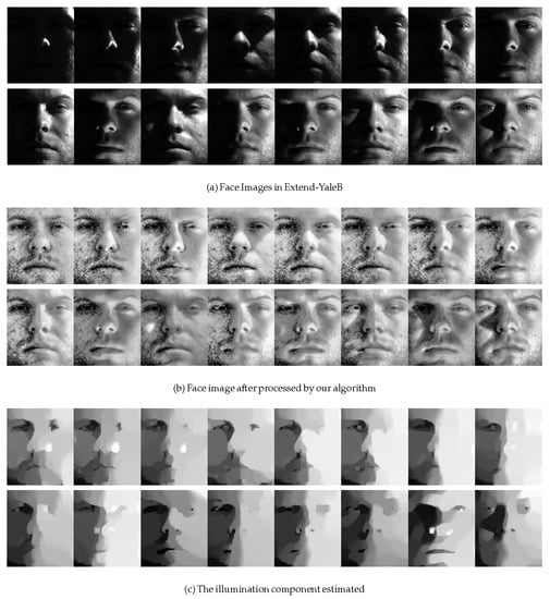
Figure 1.
The processing result of our algorithm.
In this paper, the first eight darkest images of the first entity in Extended-YaleB use internationally recognized classical lighting processing algorithms: Retina [15] (retina response algorithm), Cos [13] (discrete cosine low-pass filter), GardientFace [12] (gradient face), nlm [14] (nonlinear local smoothing algorithm), etc. It was found that almost no algorithm could effectively deal with the problem of dark-light noise. The processing effect of each classical algorithm is shown in Figure 2. It can be seen that although the algorithm proposed in this paper introduces some noise, it can basically restore the original details of the image under extremely dark-light conditions. However, other classical algorithms can only produce an illumination invariant feature map of face images, and thus, the original information of the image is lost.
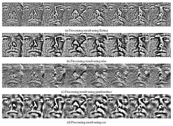
Figure 2.
The illumination removal result using state-of-the-art methods.
In order to verify the effectiveness of the algorithm in this paper for expression recognition, we selected facial expression datasets containing large illumination differences, as shown in Table 1. The CK+ dataset is used to train a CNN classifier for validation. Here, the CNN classifier was chosen as Resnet18, which is both light-weight and powerful enough for training and testing. Standard Resnet18 can be obtained from a model zoo coming together with a lot of deep learning modules in Python, i.e., Pytorch or Tensorflow. We first preprocess the images in each dataset using the illumination removal algorithm listed and then perform model training and testing, respectively.

Table 1.
The emotion classification accuracy.
The results of verification using the CNN classifier are shown in Table 1. It can be seen that illumination processing only slightly improves the accuracy of expression recognition in a single dataset but significantly improves the accuracy of expression recognition across datasets. The datasets contain rich illumination variation are marked with daggers in Table 1. We can see that the accuracy improvement of emotion classification are also most obvious in these datasets, at least 9 percent higher than raw by using our algorithm as preprocessor. Our algorithm also performs the best among compared methods. Therefore, light processing is necessary under unconstrained conditions. Among them, the algorithm based on the TV (total variance) model is generally better than the representative method LBP [20] based on feature extraction, the representative method Cone [21] based on illumination fitting, and the representative method Cos based on the principle of Lambert diffuse reflection. The authors of [13] compare the accuracy of expression recognition, although the numerical difference in accuracy is relatively weak. However, the average accuracy of the algorithm in this paper is the highest. It can be seen that the lighting processing algorithm proposed in this paper can still produce a relatively good recognition success rate when evaluating a classifier trained online with a large amount of data. This means that compared to other lighting processing algorithms, the algorithm proposed in this paper can retain more expression details for subsequent judgments.
In order to verify the impact of the illumination processing algorithm in this paper on the accuracy of expression recognition under different expression levels, we use the CK+ dataset and KDEF dataset to test the impact of the illumination recognition algorithm on the accuracy of expression recognition for different expression levels, especially for slight expression levels. The experimental results are shown in Figure 3. It can be seen that the improved algorithm based on the TV (Total Variance) model in this paper has less loss of image details than other illumination processing algorithms. It has good applicability to the expression recognition problem at a slight level and has better generalization performance for expression recognition at a slight level across datasets.
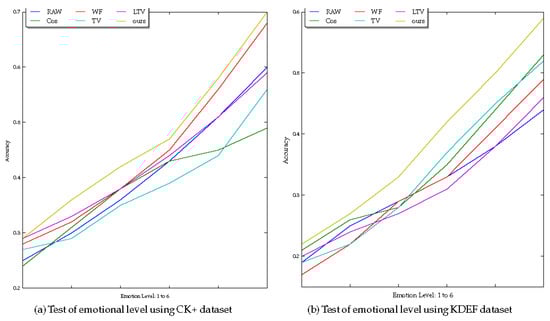
Figure 3.
Emotion level test using different illumination removal methods.
In order to observe the improvement of the illumination removal algorithm in this paper for the easily misclassified expressions, the cross-dataset verification method was used to compare the recognition effects of purely using CNN for recognition and after lighting processing on the KDEF data. As shown in Figure 4, it can be seen that although illumination processing has improved the accuracy of expression recognition to a certain extent, it has not greatly improved the recognition behavior of the CNN recognizer. That is, the facial expression categories that are more likely to be confused, such as disgust and sadness and anger and fear, are still more likely to be confused even after light processing.
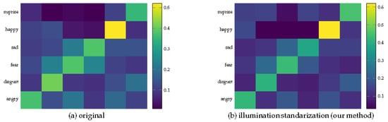
Figure 4.
The comparison of confusion matrix before and after illumination removal.
8. Conclusions
This paper attempts to remove the illumination affections of single-face grayscale images. Based on the logarithmic decomposition of the grayscale image and the Lambert reflection principle, a light intensity approximation algorithm based on the zero-order gradient regularization optimization method is proposed. The results of the experiment show that the stripping of the illumination change component by the differential statistic model of the zero-order constraint can reasonably analyze the smooth illumination component because it takes into account the extreme sparsity of the inflection point of the illumination change component in the face image. In the horizontal comparison with a series of illumination processing algorithms based on the Lambert reflection model, we believe that the illumination-invariant face images analyzed by the algorithm contain more face details, and these face details are crucial for expression recognition. The disadvantage of this model is that the resolved illumination-invariant face image still contains some noise, which can be further processed by image smoothing technology. However, since the goal of this article is to perform expression recognition on facial images, it should be more important for the expression recognition algorithm to recover the subtle details residing in the very dark or overexposure regions of the face image. Therefore, this article does not carry out further research work. In addition, for the image differential convolution kernel, this paper only considers the differential processing of the image in the vertical and horizontal directions. From the results, it can basically express the illumination change component in any direction, and if more reasonable differential convolution kernels can be added, such as diagonal directions, better results may be achieved.
Author Contributions
Writing—original draft, X.L.; Writing—review & editing, W.Y. All authors have read and agreed to the published version of the manuscript.
Funding
This research was funded by ”Training Plan for Young Backbone Teachers” of Guangdong Police College, grant number 2020QNGG02.
Data Availability Statement
Data sharing not applicable.
Conflicts of Interest
The authors declare no conflict of interest. The funders had no role in the design of the study; in the collection, analyses, or interpretation of data; in the writing of the manuscript; or in the decision to publish the results.
References
- Kim, J.; Poulose, A.; Han, D. The Extensive Usage of the Facial Image Threshing Machine for Facial Emotion Recognition Performance. Sensors 2021, 21, 2026. [Google Scholar] [CrossRef] [PubMed]
- Canal, F.; Müller, T.; Matias, J.; Scotton, G.; Sa Junior, A.; Pozzebon, E.; Sobieranski, A. A Survey on Facial Emotion Recognition Techniques: A State-of-the-Art Literature Review. Inf. Sci. 2022, 582, 593–617. [Google Scholar] [CrossRef]
- Thakur, N.; Han, C. An Ambient Intelligence-Based Human Behavior Monitoring Framework for Ubiquitous Environments. Information 2021, 12, 81. [Google Scholar] [CrossRef]
- Gage, N.; Scott, T.; Hirn, R.; MacSuga-Gage, A. The Relationship Between Teachers’ Implementation of Classroom Management Practices and Student Behavior in Elementary School. Behav. Disord. 2018, 43, 302–315. [Google Scholar] [CrossRef]
- Chen, T.; Yin, W.; Zhou, X.S.; Comaniciu, D.; Huang, T.S. Total variation models for variable lighting face recognition. IEEE Trans. Pattern Anal. Mach. Intell. 2006, 28, 1519–1524. [Google Scholar] [CrossRef] [PubMed]
- Duval, V.; Aujol, J.F.; Gousseau, Y. The tvl1 model: A geometric point of view. Siam J. Multiscale Model. Simul. 2009, 8, 154–189. [Google Scholar] [CrossRef]
- Xu, W.; Xie, X.; Lai, J. Relightgan: Instance-level generative adversarial network for face illumination transfer. IEEE Trans. Image Process. 2021, 30, 3450–3460. [Google Scholar] [CrossRef] [PubMed]
- Hu, C.H. Face illumination recovery for the deep learning feature under severe illumination variations. Pattern Recognit. 2021, 111, 107721. [Google Scholar] [CrossRef]
- Karnati, M.; Seal, A.; Bhattacharjee, D.; Yazidi, A.; Krejcar, O. Understanding Deep Learning Techniques for Recognition of Human Emotions Using Facial Expressions: A Comprehensive Survey. IEEE Trans. Instrum. Meas. 2023, 72, 1–31. [Google Scholar] [CrossRef]
- Wu, Y.; Jiang, Y.; Zhou, Y.; Li, W.; Lu, Z.; Liao, Q. Generalized Weber-face for illumination-robust face recognition. Neurocomputing 2014, 136, 262–267. [Google Scholar] [CrossRef]
- Yang, C.; Wu, S.; Fang, H.; Er, M.J. Adaptive weber-face for robust illumination face recognition. Computing 2019, 101, 605–619. [Google Scholar] [CrossRef]
- Zhang, T.; Tang, Y.; Fang, B.; Shang, Z.; Liu, X. Face recognition under varying illumination usng gradientfaces. IEEE Trans. Image Process. 2009, 18, 2599–2606. [Google Scholar] [CrossRef] [PubMed]
- Chen, W.; Er, M.J.; Wu, S. Illumination compensation and normalization for robust face recognition using discrete cosine transform in logarithm domain. IEEE Trans. Syst. Man Cybern. Part B Cybern. 2006, 36, 458–466. [Google Scholar] [CrossRef] [PubMed]
- Štruc, V.; Pavešić, N. Illumination invariant face recognition by non-local smoothing. In Proceedings of the BIOID Multicomm, LNCS 5707, Madrid, Spain, 16–18 September 2009; pp. 1–8. [Google Scholar]
- Wu, N.; Caplier, A. Illumination-robust face recognition using retina modeling. In Proceedings of the International Conference on Image Processing, Cairo, Egypt, 7–10 November 2009; pp. 3289–3292. [Google Scholar]
- Samaria, F.; Harter, A. Parameterisation of a stochastic model for human face identification. In Proceedings of the 1994 IEEE Workshop on Applications of Computer Vision, Seattle, WA, USA, 21–23 June 1994; pp. 138–142. [Google Scholar]
- Lucey, P.; Cohn, J.F.; Kanade, T.; Saragih, J.; Ambadar, Z.; Matthews, I. The extended cohn-kanade dataset (ck+): A complete dataset for action unit and emotion-specified expression. In Proceedings of the Computer Society Conference on Computer Vision and Pattern Recognition Workshops (CVPRW), San Francisco, CA, USA, 13–18 June 2010; pp. 94–101. [Google Scholar]
- Gross, R.; Matthews, I.; Cohn, J.; Kanade, T. Multi-pie. In Proceedings of the Eighth IEEE International Conference on Automatic Face and Gesture Recognition, Amsterdam, The Netherlands, 17–19 September 2008. [Google Scholar]
- Setty, S.; Husain, M.; Beham, P.; Gudavalli, J.; Kandasamy, M.; Vaddi, R.; Hemadri, V.; Karure, J.; Raju, R.; Rajan, B.; et al. Indian movie face database: A benchmark for face recognition under wide variations. In Proceedings of the 2013 Fourth National Conference on Computer Vision, Pattern Recognition, Image Processing and Graphics (NCVPRIPG), Jodhpur, India, 18–21 December 2013; pp. 1–5. [Google Scholar]
- Pan, H.; Xia, S.Y.; Jin, L.Z.; Xia, L.Z. Illumination invariant face recognition based on improved local binary pattern. In Proceedings of the Control Conference (CCC), Yantai, China, 22–24 July 2011; pp. 3268–3272. [Google Scholar]
- Georghiades, A.S.; Member, S.; Belhumeur, P.N. From Few to Many: Illumination Cone Models for Face Recognition under Variable Lighting and Pose. IEEE Trans. Pattern Anal. Mach. Intell. 2002, 23, 643–660. [Google Scholar] [CrossRef]
Disclaimer/Publisher’s Note: The statements, opinions and data contained in all publications are solely those of the individual author(s) and contributor(s) and not of MDPI and/or the editor(s). MDPI and/or the editor(s) disclaim responsibility for any injury to people or property resulting from any ideas, methods, instructions or products referred to in the content. |
© 2023 by the authors. Licensee MDPI, Basel, Switzerland. This article is an open access article distributed under the terms and conditions of the Creative Commons Attribution (CC BY) license (https://creativecommons.org/licenses/by/4.0/).