Traffic Flow Prediction Based on Dynamic Graph Spatial-Temporal Neural Network

Abstract

More accurate traffic prediction can further improve the efficiency of intelligent transportation systems. However, the complex spatiotemporal correlation issues in transportation networks pose great challenges. In the past, people have carried out a great deal of research to solve this problem. Most studies are based on graph neural networks to model traffic graphs and attempt to use fixed graph structures to obtain relationships between nodes. However, due to the time-varying spatial correlation of the transportation network, there is no stable node relationship. To address the above issues, we propose a new traffic prediction framework called the Dynamic Graph Spatial-Temporal Neural Network (DGSTN). Unlike other models that use predefined graphs, this model represents stable node relationships and time-varying node relationships by constructing static topology maps and dynamic information maps during the training and testing stages, to capture hidden node relationships and time-varying spatial correlations. In terms of network architecture, we designed multi-scale causal convolution and adaptive spatial self-attention mechanisms to capture temporal and spatial features, respectively, and assisted learning through static and dynamic graphs. The proposed framework has been tested on two real-world traffic datasets and can achieve state-of-the-art performance.

1. Introduction

Increasing vehicle ownership and travel demand have led to huge pressure on traffic management, and effectively optimizing and positioning traffic resources has become a challenge. The emergence of intelligent transportation systems (ITS) makes it very possible to solve this challenge. For example, intelligent transportation systems mainly include intelligent transportation infrastructure and data analysis algorithms such as computer vision methods for real-time monitoring of the Internet of Vehicles [1], intelligent Internet of Vehicles solutions [2,3], traffic signal controls [4], and reinforcement learning for autonomous driving [5,6], etc.

As an essential part of intelligent transportation system technology, traffic forecasting plays a vital role in solving these problems by using historical traffic data to predict future traffic conditions and helping to reduce traffic congestion by realizing effective coordination between passengers, vehicles, and roads.

Early statistical models such as support vector machine (VAR) [7], autoregressive integrated moving average (ARIMA) [8], and HA, were used for traffic prediction problems, but these models did not perform well in practice. Subsequently, some machine-learning models, such as support vector machines (SVM) [9] and the k-nearest neighbors algorithm (KNN) [10], which could model nonlinear traffic data began to emerge, but their accuracy was hindered by time-consuming and complex feature engineering. Thanks to the success of deep-learning networks in modeling time series [11,12], a large amount of literature has begun to use deep-learning models for traffic prediction problems. The most widely used is the recurrent neural network (RNN) [13,14], but it is prone to vanishing gradient problems when modeling long sequences. For spatiotemporal data, exploring the spatial correlation between data is also very important. The spatial convolution neural network (CNN) uses convolution to extract hidden information from data by dividing the research area into grids. However, this method of dividing the road network into grids is very different from the structure of the real road network [15,16,17,18]. Graph neural networks have achieved great success in processing graph topology. Time convolutional network (TCN) is an architecture that convolves in the time dimension [19,20], using extended convolution to achieve exponential-level perception fields. However, due to the use of exponential-level perception fields, they cannot effectively capture cyclic changes in traffic conditions [21]. Graph convolution neural networks (GCN) can be used because the spatial-temporal correlation of non-Euclidean space structure applies to the road network [22].

Existing models, while effective at capturing spatial-temporal correlation, still face two enormous challenges. First, we show that the spatial correlation between actual nodes changes dynamically over time rather than being static and invariant. Traffic conditions detected by a specific sensor are difficult to capture. As can be seen in Figure 1a, for example, the spatial correlation between nodes A and B is very high in the morning hours but then weakens between nodes C and D during the afternoon. Second, most models typically use a predefined static graph structure to describe the actual road network relationship; the graph of the adjacency matrix constructed using Euclidean distance does not really reflect the spatial relationship of the road network, e.g., Figure 1b shows that nodes C and D are two nonadjacent sensor nodes which are highly correlated spatially.

To solve the above problems, we propose a new framework to solve the traffic flow problem: the Dynamic Graph Spatial-Temporal Neural Network (DGSTN) is used to predict the traffic flow of each sensor in the traffic network. We designed a set of adaptive graphs, including static graphs that can capture real node correlations in road networks and dynamic graphs that capture dynamic spatial correlations. In addition, for the model, temporal characteristics were captured by constructing multi-scale temporal convolutions, and time-varying spatial characteristics were captured according to an adaptive spatial self-attention mechanism and the proposed static topology and dynamic information graphs. Specifically: the main contributions of this paper are as follows:

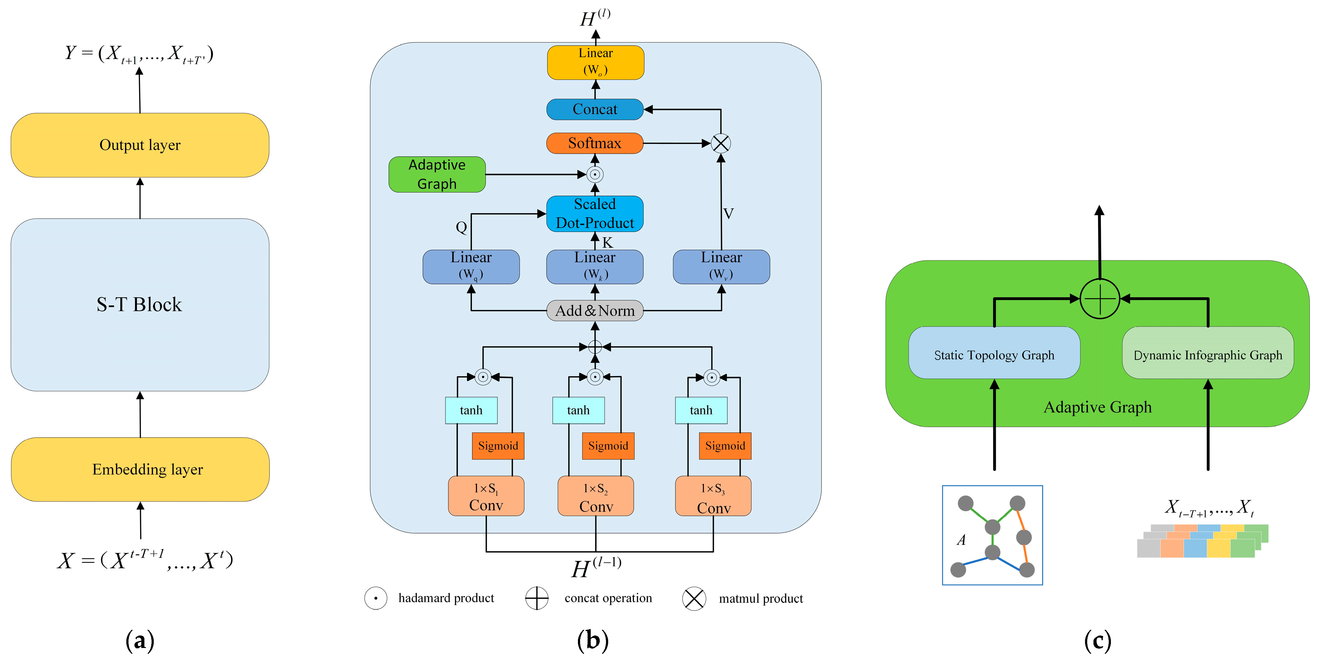
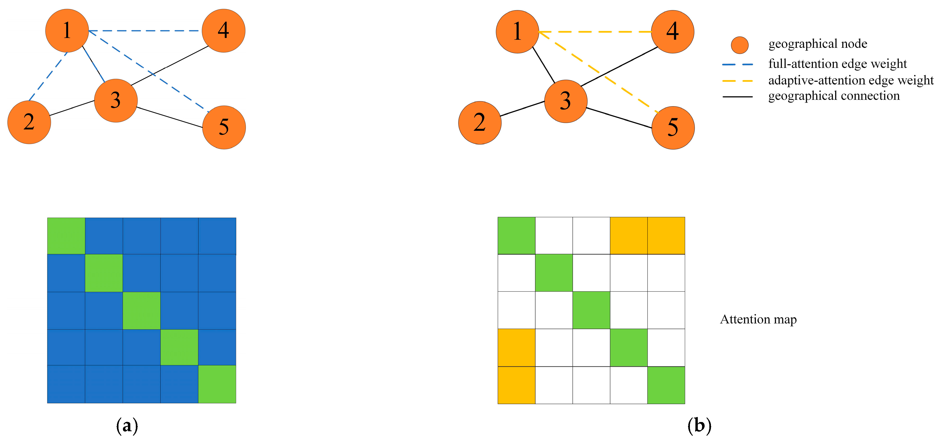
• A multi-scale time-gated convolution is proposed to capture different temporal finesse and, based on an improved adaptive spatial self-attention mechanism, the node correlation of the real spatial relationship is calculated.
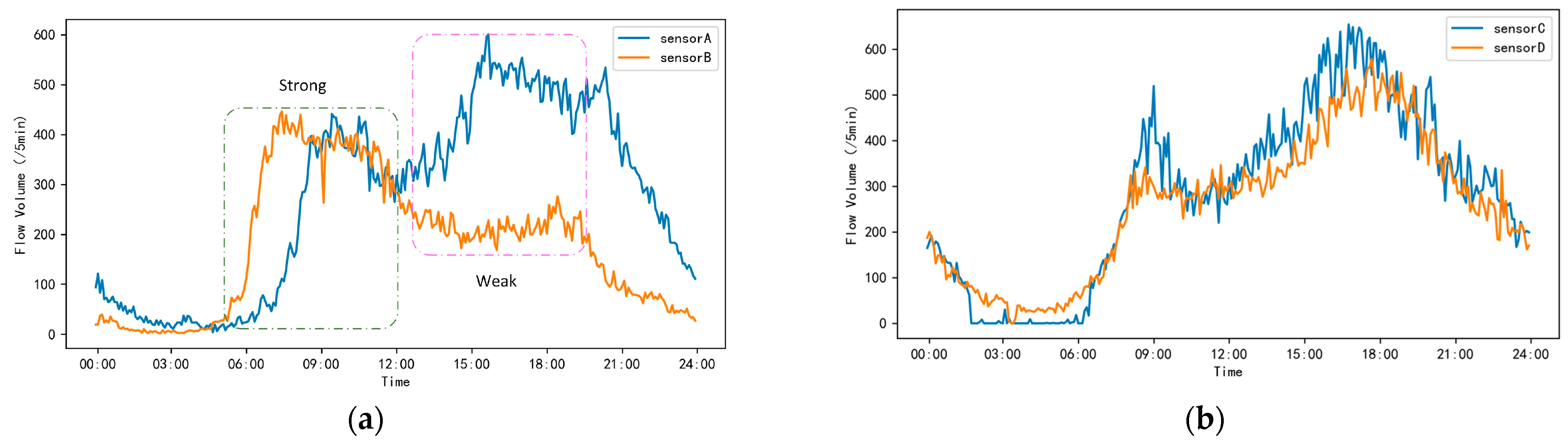
• The design is a set of adaptive graphs: a static topology graph combined with an adjacency matrix as prior information and an adaptive embedding matrix to capture real node dependencies. By capturing the similarity of changes in flow information, a set of dynamic information graphs is constructed to obtain a dynamic spatial correlation.
• Results tested on two real-world datasets and show that the framework proposed in this paper achieves the best results when compared with various baselines.

2. Literature Review

2.1. Space-Time Traffic Forecast

The prediction of traffic flow is a fundamental problem in intelligent transportation and has been extensively studied by many researchers over time, with applications in a wide range of areas. Initial research was focused on statistically based methods including VAR [7], ARIMA [8], and HA. These models are underpinned by mathematical theory, but they rely on the assumption of linearity in the prediction task, which is not consistent with the nonlinear nature of the traffic data, leading to poor prediction results. Models based on machine learning may be a good solution to this problem e.g., SVM [9] and KNN [10], but good results rely on high-quality manual feature generation, which undoubtedly leads to complex and time-consuming modeling. Models based on deep learning perform well in other domains, automatically extracting network features from a given dataset, obviating the need for manual feature generation, and alleviating modeling complexity. The success of convolutional neural networks (CNN) in computer vision tasks has been so great that some academics have used them for traffic [13,14,23]. However, modeling methods that use mesh partitioning for convolutional operations are not, on their own, sufficient to capture the topology of road networks. The RNN-based model is very suitable for sequence data. It is a widely used practice to capture temporal and spatial features by combining long Short-term Memory (LSTM) and convolutional neural networks [14]. However, these methods can only use off-the-shelf solutions without exploring the correlation of different regions, and it is more challenging to preserve long-term information for long-sequence problems in recursive sequence models such as RNN and LSTM.

2.2. Graph Convolution

The recent emergence of graph convolutional networks is well suited to traffic prediction tasks, given that traffic path networks are natural graph topologies. Much of the work is based on modeling in either the time and space dimensions separately, or in the space-time dimension. Since traffic data must be considered correlated in both time and space dimensions, a common approach to combining convolution with recursive models such as RNNs is to use convolution in place of the matrix multiplication operation of recursive models with convolution on a local spatial-temporal graph [10,18]. Most tasks in spatial dependency capture use predefined graphs built based on Euclidean distances to capture spatial dependencies, but in real-world traffic networks two sensors that have similar Euclidean distances may not exhibit strong spatial dependencies for certain specific purposes (intersections, roadway closures, two opposite lanes, roadway area functions). To address this issue, refs. [16,24] make use of adaptively learnable graph structures to capture the real spatial dependencies.

2.3. Attention Mechanisms

Attention mechanisms first appeared in the modeling of problems for natural language processing and are now used in a wide range of domains [25,26], providing efficient improvements to many tasks [27,28]. One immediate goal of using attention mechanisms is to score the various dimensions of the input and then weigh the features based on their scores to highlight the impact that important features have on downstream models or modules. The basic idea of the attention mechanism is as follows. Numerous models that have emerged in the field of traffic prediction also prove the efficacy of attention, such as [29,30,31].

Attention becomes self-attentive when the query, the key, and the value are the same, and in sequential tasks, it can parallelize processing and consider information from the global sequence more efficiently and quickly. The emergence of multi-headed attention [32], which can learn the correlation of different subspaces, allows the self-attention mechanism to bring greater flexibility and modeling ease to the problem compared to CNN and RNN.

3. Materials and Methods

3.1. Problem Formulation

Definition 1.

(Road Network). The road network can be viewed as a graph $G=(V,E,A)$, where $V=\{v_1,\dots ,v_N\}$ is a set of $N$ nodes ($N= \left|V\right|$), $E$ is an edge set, and A is the adjacency matrix of the traffic road network $G$.

Definition 2.

(Traffic Flow Tensor). We use $X_t\in {ℝ}^{N\times F}$ to represent the traffic flow of N nodes in the traffic network at time $t$, $F$ is a feature dimension. We use $X=(X_1,X_2,\dots ,X_T)\in {ℝ}^{T\times N\times F}$ to represent the traffic flow of all nodes in the road network at T time slices.

The goal of traffic flow forecasting is to predict the future flow of the entire traffic system through given historical flow information. Formally, our goal is to learn a function f to predict the traffic flow of $T^{\prime }$ time steps in the future given the traffic flow observations of $T$ historical time steps.

$$f:[X_{(t-T+1)},\dots ,X_t;G]\to [X_{(t+1)},\dots ,X_{(t+T^{\prime })}]$$

(1)

3.2. Dynamic Graph Spatial-Temporal Neural Network

We show the framework of DGSTN, which consists of an embedding layer, S-T block, and an output layer, in Figure 2a. The input to the model is historical traffic data $X=[X_{(t-T+1)},\dots ,X_t]\in {ℝ}^{T\times N\times F}$, and the output is to predict traffic flow $Y=[X_{t+1},\dots ,X_{t+T^{\prime }}]\in {ℝ}^{T\times N\times C}$ over a period of time in the future. The input of each space-time block is $H^{(l-1)}\in {ℝ}^{T\times N\times D}$, and the output is $H^{(l)}$. The details are shown in Figure 2b.

3.2.1. Adaptive Graph

In this section, we describe how to leverage a given information graph $G=(V,E,A,X_{t-T:t})$ so static topology graphs and dynamic information graphs can learn from static topology and dynamic traffic information, respectively. Figure 2c shows the specific details of the adaptive graph.

Static Topology Graph

To solve the difficulty of capturing globally valid information using predefined graphs in most current models, we propose a static topology graph that learns the adjacency matrix of the optimal graph. It learns the implicit information that cannot be captured by predefined graphs, and then projects the hidden relationship into the predefined adjacency matrix to achieve complementary information. First, the initialization of the predefined adjacency matrix graph plays an important role in the learning of the adaptive graph, and we define the initialization as: $L=I+D^{-\frac{1}{2}}{A}_{}{D}^{\frac{1}{2}}$, where $A$ is the adjacency matrix, $I$ is the unit matrix, $D\in {ℝ}^{N\times N}$ is the degree matrix, and $D_{ii}={\displaystyle {\sum }_i{A}_{ij}}$ is constructed as. The specific definition is as follows:

$$A_1=Relu(E_1{E}_2^{\top }+Diag(\Lambda ))$$

(2)

Here, $E_1,E_2\in {ℝ}^{N\times F^{\prime }}$, $\Lambda \in {ℝ}^N$ is the learnable parameter, $N$ is the size of the node, and $F^{\prime }$ is the dimension of the learnable parameter, where $F^{\prime }\ll N$. By multiplying $E_1$ and $E_2$, one can generate a sparse graph, where $Diag(\Lambda )$ is used to generate the weights of the diagonal positions and $Relu$ is used to eliminate the weak connection after adding the two. Note that no prior knowledge is required for the sparse matrix $A_1$ here, and all parameters are learned end-to-end by stochastic gradient descent. Adaptive modules are then used to adaptively aggregate predefined and learnable sparse matrices.

$$S=Sigmoid(Cov(A_1+L))$$

(3)

$$A_3=S\odot A_1+(1-S)\odot L$$

(4)

Here, we perform an adaptive aggregation operation on the resulting sparse matrix $A_1$, the predefined matrix $L$, $Sigmoid$ is a nonlinear activation function and $Cov$ is a convolutional layer of 1 × 1, where $\odot$ represents element multiplication. Since the new matrix is obtained by adaptive aggregation based on predefined graphs $A_1$ and learnable sparse matrices $L$, it not only retains the prior features of the predefined graphs $L$, but also learns node features through training, ensuring faster convergence in the iterative process.

$$A_s=D_3^{-\frac{1}{2}}{A}_3{D}_3^{-\frac{1}{2}}$$

(5)

The normalization operation is performed on the final matrix obtained.

Dynamic Information Graph

The spatial correlation between different nodes will change with time, so it is necessary to use node information to mine the change in spatial correlation. First, for the given node information $X\in {ℝ}^{T\times N\times F}$, we need to upgrade the feature dimension to D dimension; the specific formula is as follows:

$$S=FC(X)\in {ℝ}^{T\times N\times D}$$

(6)

In this formula, $FC(·)$ is a fully connected network and $S$ represents the node attributes after linear mapping. To capture the dynamically changing spatial correlation over $T$ time lengths, we need to use a one-dimensional dilated convolution to perform convolution operations on the time dimension:

$$DC(S)=({\displaystyle \sum _{t=d\times (k-1)}^T{\displaystyle \sum _{K=0}^{K-1}{w}_k·S_{t-d\times k}}})$$

(7)

Equation (7) represents a one-dimensional dilated convolution operation. We can stack multiple dilated convolutional layers and aggregate the time dimension to arrive at the formula:

$$M=D{C}_3(D{C}_2(D{C}_1(S)))$$

(8)

Through formula (8), we convert $S\in {ℝ}^{T\times N\times D}$ into $M\in {ℝ}^{N\times D}$, where the overall parameter of the convolution kernel is $w\in {ℝ}^{T\times D\times D}$. In our model, cosine similarity is used to calculate the spatial correlation between two nodes. Therefore, the relationship between two nodes can be expressed as:

$$S_{ij}=\frac{M_i·M_j^{\top }}{‖M_i‖‖M_j^{\top }‖}$$

(9)

Here, $S_{ij}$ represents the similarity between node $i$ and node $j$. The higher the similarity, the stronger the spatial dependence and the higher the spatial correlation. Furthermore, the spatial dynamic graph $A_d$ can be expressed as the following form:

$$A_d=Softmax(Relu(S_{ij}))$$

(10)

The $Relu$ activation function here can eliminate negative connections and enhance the nonlinear capability, while the $Softmax$ function is used to normalize the dynamic information graph.

3.2.2. Multi-Scale Gated Time Convolution

Compared with recursive units, convolutional operations do not require sequential calculations, which can save a great deal of computational time. Compared to self-attention mechanisms that require a large number of parameters, they only require a few parameters, making the models more lightweight. In contrast to the design of TCN, we designed a multi-scale time convolution which consists of three GTU-gated convolutions with a different receptive field.

The input to the time-gated convolutional network is $Z^{(l)}\in {ℝ}^{T\times N\times D}$, where $l$ is the number of ST layers. The size of the convolutional kernel is $\theta \in {ℝ}^{K\times D\times 2D}$, and here the output of the network is $Z^{\prime (l)}=\theta \ast Z^{(l)}\in {ℝ}^{N\times (T-(S-1))\times 2D}$ and the whole cell can be defined as follows:

$$Z^{(l)}=\sigma (Z^{\prime (l)})\odot Tanh(Z^{\prime (l)})$$

(11)

Here $\sigma$ stands for the $Tanh$ activation function and $\odot$ for the Hadamard product. We employ a multi-scale gated convolution module to capture the dynamic temporal information of the traffic by adjusting the size of the convolution kernel to obtain different perceptual fields, which are used to capture the long-term and short-term temporal dependencies. The multi-scale GTU can be represented as follows:

$$Z_{out}^{(l)}=Norm({\theta }_1\ast {\mathrm{Z}}^{(l)}+{\theta }_2\ast {\mathrm{Z}}^{(l)}+{\theta }_3\ast {\mathrm{Z}}^{(l)})$$

(12)

Here $1\times k_1$,$1\times k_2$, and $1\times k_3$ are the sizes of the convolution kernels of ${\theta }_1$, ${\theta }_2$, and ${\theta }_3$, respectively. The operation fuses the features obtained from the GTU with three different receptive fields, resulting in a feature with a size of $3T-(k_1+k_2+k_3-3)$.

3.2.3. Spatial Attention

When modeling spatial-temporal data, spatial correlations change dynamically at different time steps. The most direct way to capture this feature is to use a fully connected spatial attention mechanism (FSA) to obtain the attention of all nodes at different times. However, in real road networks, many nodes are not directly connected due to geographical location or weak correlation. To address this issue, we employ an adaptive spatial attention method that captures the dynamic spatial correlation between nodes with realistic relationships. Figure 3 demonstrates the difference between fully connected spatial attention and adaptive spatial attention.

For fully connected spatial attention, it is first necessary to obtain the query, key, and value vectors of the self-attention mechanism:

$$Q_t^{(S)}=X_t{W}_Q^S,K_t^{(S)}=X_t{W}_K^S,V_t^{(S)}=X_t{W}_V^{(S)}$$

(13)

Here, $W_Q^S$, $W_K^S$, and $W_V^S\in {ℝ}^{D\times D\prime }$ are a set of learnable parameters and $D^{\prime }$ is the dimensions of query, key, and value. Next, the dependencies between nodes are computed in the spatial dimension, and the attention scores of all nodes at time $t$ are computed:

$$A_t^{(S)}=\frac{(Q_t^{(S)}){(K_t^{(S)})}^{\top }}{\sqrt{D^{\prime }}}$$

(14)

At different time steps, the attention scores $A_t^{(S)}$ are different between each node, which can dynamically capture the spatial correlation. Further, the output of spatial self-attention can be obtained by multiplying the attention score $A_t^{(S)}$ with the Value matrix:

$$FSA(Q_t^{(S)},K_t^{(S)},V_t^{(S)})=Softmax(A_t^{(S)})V_t^{(S)}$$

(15)

The above formula is the standard full-spatial attention, where all nodes are related to each other. The adaptive spatial attention we adopted designs a mask matrix $M$ that performs a masking operation on nodes with less spatial correlation at each time step, and only considers the correlation between nodes with a greater relationship to reality. When the correlation is less than the threshold, this means that the correlation between the two nodes is small so the attention between the two nodes is covered up, and the attention score is set to $-\infty$. Furthermore, the attention score $A_t^{(S)}$ can be further tuned by multiplying it with the adaptive graph $A_{adap}$. Therefore, adaptive spatial attention can be expressed as follows:

$$ASA({\mathrm{Q}}_t^{(S)},K_t^{(S)},V_t^{(S)},A_{adap})=Softmax((A_t^{(S)}+M)\odot A_{adap})V_t^{(S)}$$

(16)

The symbol $\odot$ here represents the Hadamard product. Adaptive spatial attention accomplishes adaptive modeling of spatial correlations between real nodes. Multi-head spatial attention can be expressed as:

$$MASA=\oplus (AS{A}_1,AS{A}_2,\dots ,AS{A}_h)W_O$$

(17)

By introducing a multi-head spatial-attention mechanism, where parallel attention heads are stitched together, hidden spatial dependencies can be captured from various subspaces.

Since the multi-headed attention mechanism completely discards the convolution and recursive operations, it is necessary to add a mark to each input to represent the timing and position relationship. To this end, we design a spatial embedding (SE) to better capture spatial dependencies. The adaptive graph $A_{\mathrm{adap}}$ learned by the graph learning module can be initialized to obtain the spatial embedding $S_E\in {ℝ}^{N\times N}$, which can capture the connectivity and distance relationship between nodes, and it can transform the spatial and temporal embeddings linearly and along the temporal and spatial dimensions to generate $S_E\in {ℝ}^{T\times N\times D}$.

3.2.4. Input and Output Layer

The input layer is used to map the input node to a high-dimensional space, and a 1 × 1 convolution is used to convert the data dimension into $X\in {ℝ}^{T\times N\times D}$. To realize the function of multi-step prediction, the output layer uses two 1 × 1 convolutions to convert the hidden dimension into the required dimension $\widehat{X}\in {ℝ}^{T\prime \times N\times C}$. The loss function uses the mean absolute error between the predicted value $Y=[{\widehat{X}}^{t+1},\dots ,{\widehat{X}}^{t+T}]$ and the true value $X=[X^{t-T+1},\dots ,X^t]$:

$$L=\frac{1}{T}{\displaystyle \sum _{t\prime =t+1}^{t\prime =t+T}{\left|{\widehat{X}}_{t\prime }-X_{t\prime }\right|}_1}$$

(18)

4. Results and Discussion

In this section, we present the experimental results of the DGSTN and baseline on two spatiotemporal datasets, using multiple evaluation indicators for comprehensive evaluation. During the study, we conducted ablation experiments on the model to analyze the effectiveness of each component and adaptive graph.

4.1. Datasets

To evaluate the performance of the proposed model, we conducted experiments on two real-world datasets: PeMS04 and PeMS08. PeMS is a unified database of traffic data collected by California transportation companies and partners on California highways, reporting data every 30 s. The dataset descriptions are as follows:

• PeMS04: Traffic data collected by Caltrans Performance Measurement System (PeMS) from 307 detectors in the San Francisco Bay Area from 1 January 2018 to 28 February 2018.
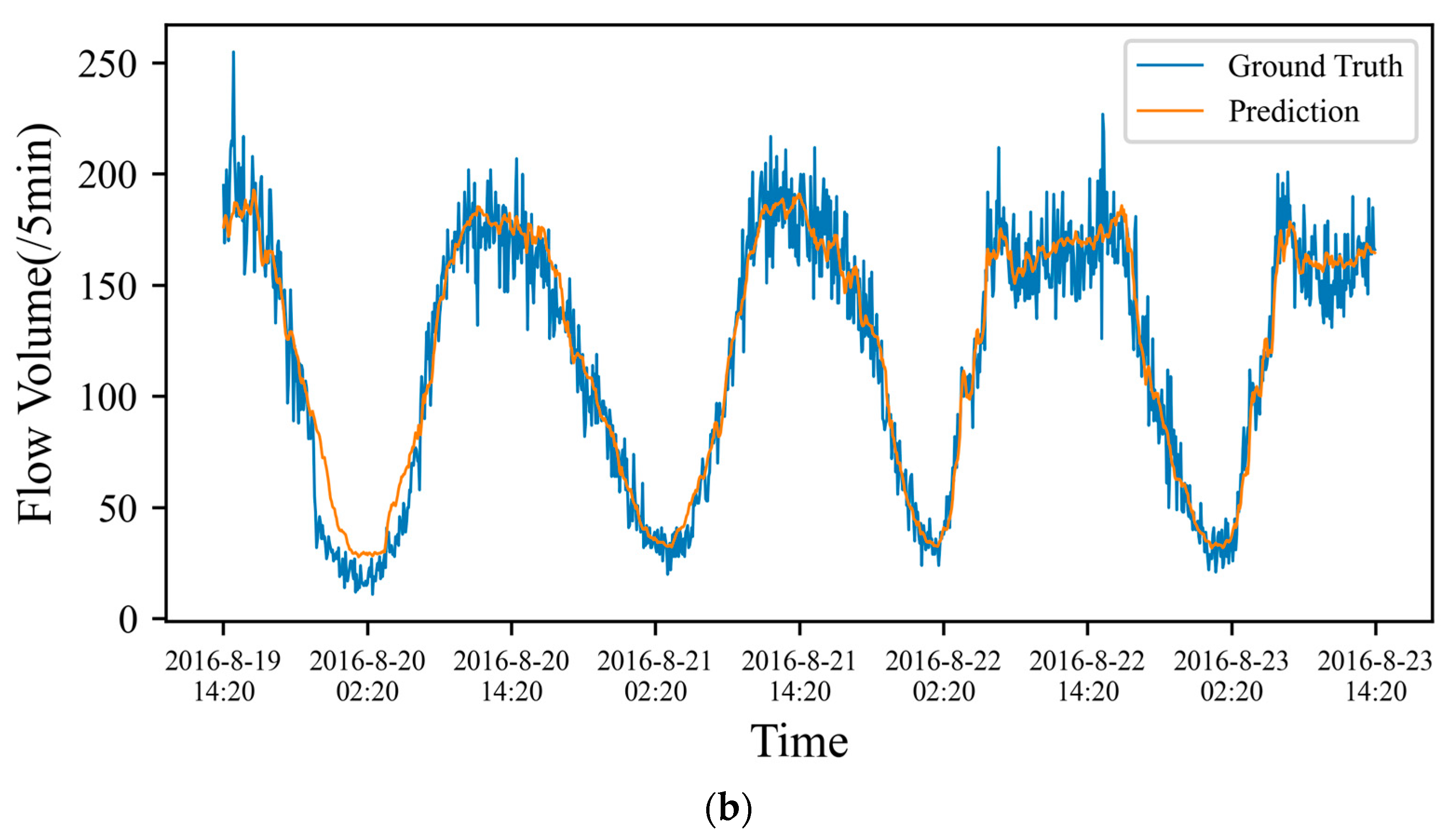
• PeMS08: Traffic information collected by the Caltrans Performance Measurement System (PeMS) from 170 detectors in the San Bernardino area from 1 July 2016 to 31 August 2016.

The traffic flow data of the two datasets is recorded every 5 min, with a total of 288 pieces of data per day. The missing values in the above two datasets are filled in by linear interpolation, and the training is made more stable by normalizing the dataset by the standard normalization method $x^{\prime }=x-mean(x)$. In the forecasting process, this paper uses one hour’s historical data to predict the next hour’s data; that is to say the historical data of 12 time steps is used to predict the future data of the next 12 time steps. The two datasets are divided into training, validation, and test sets in chronological order, with a segmentation ratio of 6:2:2.

Table 1. Dataset description for experiments.

Datasets	Nodes	Edges	Time Steps	Time Range
PeMS04	307	340	16,992	1 January 2018–28 February 2018
PeMS08	170	295	17,856	1 July 2016–31 August 2016

summarizes the key information of these two datasets.

4.2. Baseline Method

We compared the proposed framework with baseline methods, including classical methods and advanced neural network methods.

• HA: Historical average value, which uses traffic flow data from the past period and calculates its average value to achieve prediction.
• ARIMA [8]: The Kalman filter autoregressive comprehensive moving-average model is a classic time-series prediction model.
• FNN: feedforward neural network, the neural network of multiple hidden layers.
• LSTM: Due to its memory function, LSTM can use long sequence information to construct learning models.
• DCRNN [13]: Diffusion convolutional recurrent neural network combines a recurrent neural network with diffusion convolution to model the relationship between traffic inflow and outflow.
• ASTGCN [15]: An attention-based spatiotemporal graph convolutional network for traffic flow prediction. By overlaying attention layers and convolutional layers, temporal and spatial features in the data were proposed to obtain more effective temporal and temporal features.
• STSGCN [18]: Spatiotemporal synchronous graph convolutional network. To more effectively capture complex local spatiotemporal correlations more, a spatiotemporal synchronization graph modeling mechanism is proposed.
• GWN [16]: Graph WaveNet for deep spatiotemporal graph modeling. A graph convolutional architecture, which proposes an adaptive graph to capture spatial correlations and uses diffusion convolution to capture temporal relationships, is suggested.
• AGCRN [24]: An adaptive graph convolutional recursive network for traffic volume prediction. This modifies commonly used graph convolutions through node-adaptive parameter learning and adaptive graph-generation modules, and combines graph convolution with GRU to explore spatiotemporal correlations in data.
• ASTGNN [30]: The learning dynamics and heterogeneity of spatiotemporal map data for traffic prediction. This model adopts a self-attention mechanism to capture features in both temporal and spatial dimensions.

4.3. Experiment Settings

All experiments in this paper were conducted on a machine equipped with NVIDIA GeForce 3060ti and 16 GB of RAM. The models in this paper were implemented using Windows 11, Py-Torch 1.17, and Python 3.9. Similar training settings to those in [33,34] were used, and were trained using an Adam optimizer with learning rate of 0.001, a batch size of 32, and an epoch of 100, and using an early stopping strategy to prevent overfitting, both in training the baseline model and the model proposed in this paper. The layer of DSTGN was set to 3, and the embedding dimension was set to 128. The convolution kernels $k_1$, $k_2$ and $k_3$ of the gated temporal convolution were set to 3, 5, and 8, respectively, and the number of heads of spatial multi-head attention was set to 8.

4.4. Performance Comparison

We used three widely used metrics: mean absolute error (MAE), root-mean-square error (RMSE), and mean absolute percentage error (MAPE), to measure the predictive performance of the model. We compared the predictive performance of the proposed model with the baseline model on the PeMS04 and PeMS08 datasets.

Table 2. The average prediction performance for the next hour of DGSTN and other different methods on two real-world datasets.

Model	PeMS04			PeMS08
	MAE	RMSE	MAPE (%)	MAE	RMSE	MAPE (%)
HA	24.50	39.83	16.58	21.19	36.64	13.79
ARIMA	31.55	47.57	21.40	25.27	37.77	15.539
FNN	26.82	41.56	19.98	22.40	34.71	22.47
LSTM	25.69	40.02	17.76	20.24	31.84	12.78
DCRNN	23.05	35.72	15.97	18.29	28.61	11.62
ASTGCN	21.99	34.97	14.49	18.53	28.69	11.21
STSGCN	21.41	34.28	14.49	17.79	27.37	11.70
GWN	20.82	32.35	14.70	15.86	24.97	10.13
AGCRN	19.68	32.27	13.04	16.90	26.77	10.53
ASTGNN	19.33	31.20	13.14	15.81	25.03	9.97
DGSTN	18.88	30.86	12.47	15.27	24.33	9.82

shows the average performance of the model presented in this paper and the baseline model over the next hour. Our model achieves the best performance at different moments. (1) First, it can be found that both our model and the deep-learning model are ahead of the traditional methods HA and ARIMA, something which shows that deep learning is very effective in modeling time-series forecasting. (2) Compared with the deep-learning model LSTM which only models the time dimension, our model and some deep-learning models which consider graph structure information are ahead, indicating a strong spatial-temporal dependency in the spatial-temporal sequence. (3) Our model and the self-attention-based ASTGCN and AASTGN models outperform recurrent networks such as DCRNN and LSTM in terms of performance, suggesting that capturing dynamic spatial-temporal correlations is highly necessary. (4) Our model and GWN which consider the graph relationship are better than the graph model DCRNN and STSGCN in terms of effect, indicating that the adjacency graph constructed using only Euclidean distance cannot reflect the real spatial relationship, and that exploring the real node relationship can improve model performance. (5) Compared with GWN and AGCRN, which only consider static node relationships, our model also considers dynamic node relationship changes, learns time-varying spatial characteristics, and demonstrates more powerful performance. (6) Compared with models such as ASTGCN and ASTGNN which use self-attention mechanisms, our model uses spatial attention to interact with the adaptive graph structure proposed in this paper and adaptively selects relevant nodes for spatial attention calculations. The performance of the model is improved, and the effectiveness of considering node relationships is further demonstrated. (7) Compared with the baselines, our model has a significant lead in the long-term prediction effect.

Table 3. The prediction effect of DGSTN and other methods on PeMS04 datasets with different step lengths for the next hour.

Model	MAE			RMSE			MAPE (%)
	15 min	30 min	60 min	15 min	30 min	60 min	15 min	30 min	60 min
HA	22.03	25.98	34.92	34.42	40.01	52.03	16.83	19.27	25.51
LSTM	21.13	24.90	33.40	33.25	38.54	49.96	14.26	16.98	23.89
DCRNN	19.95	22.64	28.15	31.30	34.97	42.29	13.60	15.57	19.97
ASTGCN	19.84	21.62	25.99	31.62	34.27	40.60	13.20	14.34	16.87
STSGCN	19.80	21.24	24.20	31.93	34.04	38.18	13.51	14.24	16.31
GWN	19.03	20.68	23.88	29.87	32.15	36.53	13.03	14.82	17.38
AGCRN	18.87	19.59	21.07	30.89	32.13	34.36	12.55	13.00	13.89
ASTGNN	18.17	19.45	21.30	29.53	31.57	34.36	12.55	12.77	13.95
DGSTN	18.04	19.09	20.55	29.59	31.53	33.81	12.11	12.74	13.72

and

Table 4. The prediction effect of DGSTN and other methods on PeMS08 datasets with different step lengths for the next hour.

Model	MAE			RMSE			MAPE (%)
	15 min	30 min	60 min	15 min	30 min	60 min	15 min	30 min	60 min
HA	18.28	21.45	29.81	28.23	33.26	44.40	20.33	21.86	26.46
LSTM	16.57	19.61	26.58	25.88	30.76	40.29	10.30	12.29	17.14
DCRNN	15.79	18.02	22.49	24.45	28.08	34.48	10.01	11.42	14.31
ASTGCN	16.35	18.40	22.25	25.25	28.43	33.77	10.11	11.06	13.10
STSGCN	16.40	17.68	20.15	25.10	27.35	30.92	10.91	11.52	13.01
GWN	14.49	15.85	17.91	22.75	25.10	28.21	9.18	10.10	11.31
AGCRN	15.45	16.68	19.53	24.25	26.43	30.78	9.63	10.34	12.19
ASTGNN	14.23	15.78	18.25	22.47	24.99	28.55	9.23	9.92	11.22
DGSTN	14.26	15.30	16.92	22.46	24.41	26.89	9.20	9.76	10.84

, Figure 4 show the changes which occur in the prediction performance of various methods as the prediction interval increases in the two datasets.

To understand and evaluate the predictive performance of the model more intuitively, we visualized the predictive effect of the model. We chose sensors No. 7 and No. 157 in the PeMS08 data set and took the real data for 24 h a day from the No. 7 sensor to visualize the prediction effect of STSGCN, ASTGCN, and the model proposed in this paper. It can be seen from Figure 5a that STSGCN has a lower degree of fitting with ASTGCN, and DSTGN has a closer effect on the prediction of traffic flow than the accurate prediction. Compared with the other two models, the predicted situation of DSTGN is more in line with the actual situation during the two periods of 3:00 pm to 6:00 pm and 6:00 pm to 8:00 pm. At the same time, while our model is good at capturing the inherent patterns of time series, it can also effectively avoid over-fitting problems. For example, in Figure 5b we visualize the accurate and predicted traffic flow data recorded by sensor No. 157 from 19 August 2016 to 23 August 2016. It can be seen intuitively that the sensor generally reaches the low peak of the day at around 2:00 pm and reaches the highest peak around 2:00 pm. At 2:00 pm on 19 August 2016, the traffic flow suddenly had an abnormal increase. That night it suddenly decreased abnormally, resulting in a low peak at around 2:00 am on 20 August 2016, compared to other days, with lower peaks and valleys. However, our model did not firmly fit the abnormal changes in that day’s data. Our model achieves impressive predictions, but some local predictions may need improvement due to random noise.

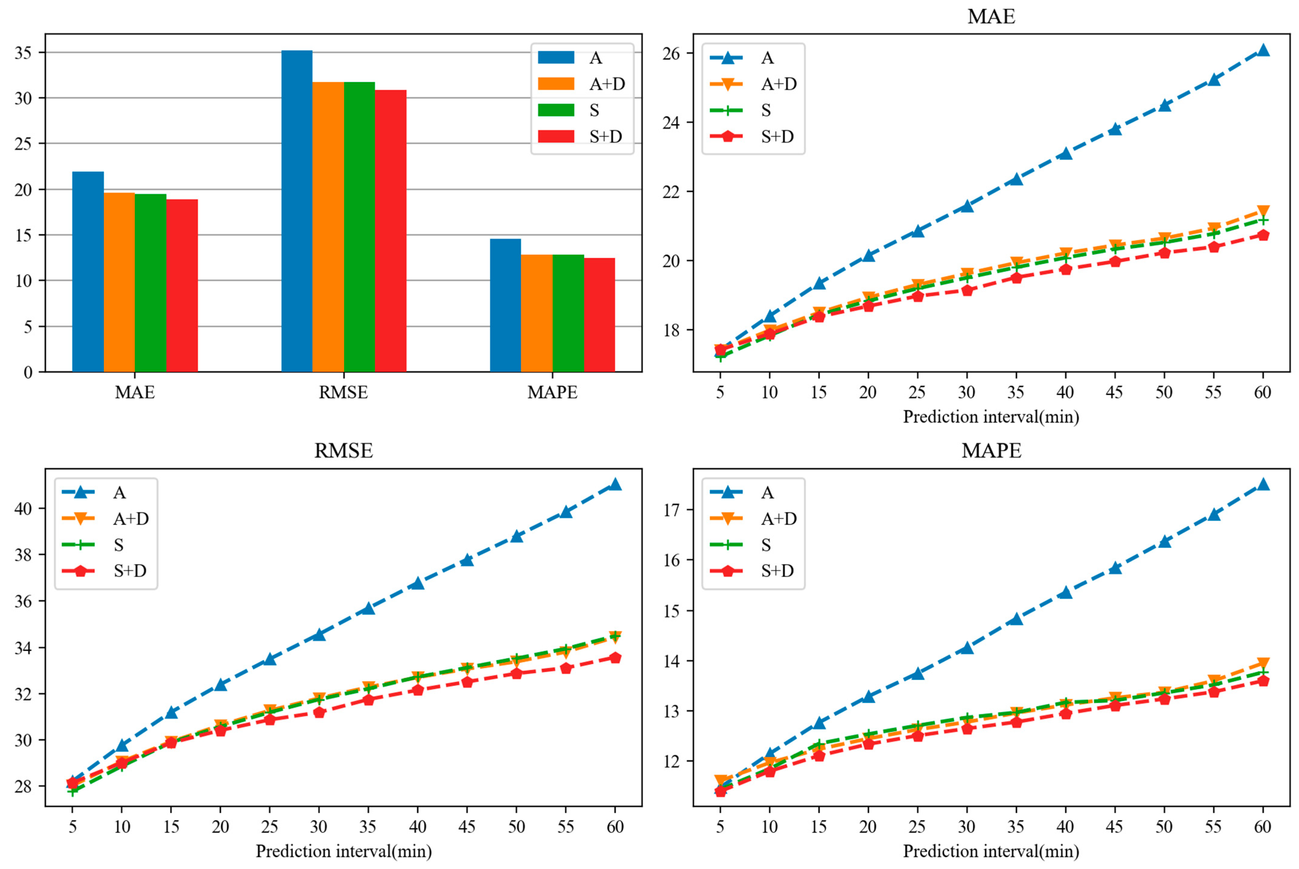
4.5. Ablation Experiment

For this section, we conducted ablation experiments on the adaptive graph structure on the PeMS-04 dataset to verify the effectiveness of the model. First, we defined three different graph structures: static matrix (S), dynamic information matrix (D), and adjacency matrix (A). For the above three different graph structures, we made different combinations.

Figure 6 shows the detailed results of the model’s average results for one hour and predictions for each time slice under different graph structure combinations. In the prediction effect of PeMS04 data set, the combination of static topology matrix and dynamic information matrix shows the best effect, while the case of only considering the adjacency graph is the worst, which further shows that only using the distance of each node is not enough to judge the relationship strength of nodes; further exploring the effective node relationships is very effective. Based on the adjacency graph, adding dynamic graph information leads to the effect being greatly improved, something which shows that it is very effective to construct a dynamic graph by introducing traffic similarity and further proves the necessity of capturing the dynamic characteristics of node traffic. The graph structure composed solely of static graphs has a greatly improved effect compared with the adjacency matrix, which shows the effectiveness of mining hidden relationships between nodes. The adaptive graph structure composed of static graphs and dynamic graphs works best, further proving the necessity of capturing hidden spatial relationships and flow characteristics between various nodes. In short, the design of each graph has a positive impact on performance improvement.

4.6. Model Efficiency Study

In this section, we compared the computational efficiency of the model with the training time and inference time, and the results are shown in

Table 5. The computation cost on the PeMS04 dataset.

Model	Computation Time
	Training (s/Epoch)	Inference (s)
DCRNN	93.20 s	11.91 s
STSGCN	196.98 s	26.69 s
ASTGCN	84.39 s	9.45 s
ASTGNN	101.37 s	47.91 s
DGSTN	74.01 s	9.99 s

. AASTGN obtains the optimal computational efficiency. Unlike DCRNN which uses a recurrent network, AASTGN can directly generate all predictions so the running speed is faster than DCRNN. STSGCN obtains the space-time graph information for adjacent time steps for modeling, and needs to be calculated at each time step, while AASTGN uses adaptive node embedding and learns the dynamic characteristics of node information, and can learn faster. ASTGCN and ASTGNN use the self-attention mechanism, which results in a substantial increase in computing speed. Compared with the previous two models, DGSTN has better computational costs for improved adaptive spatial attention and multi-scale temporal convolution.

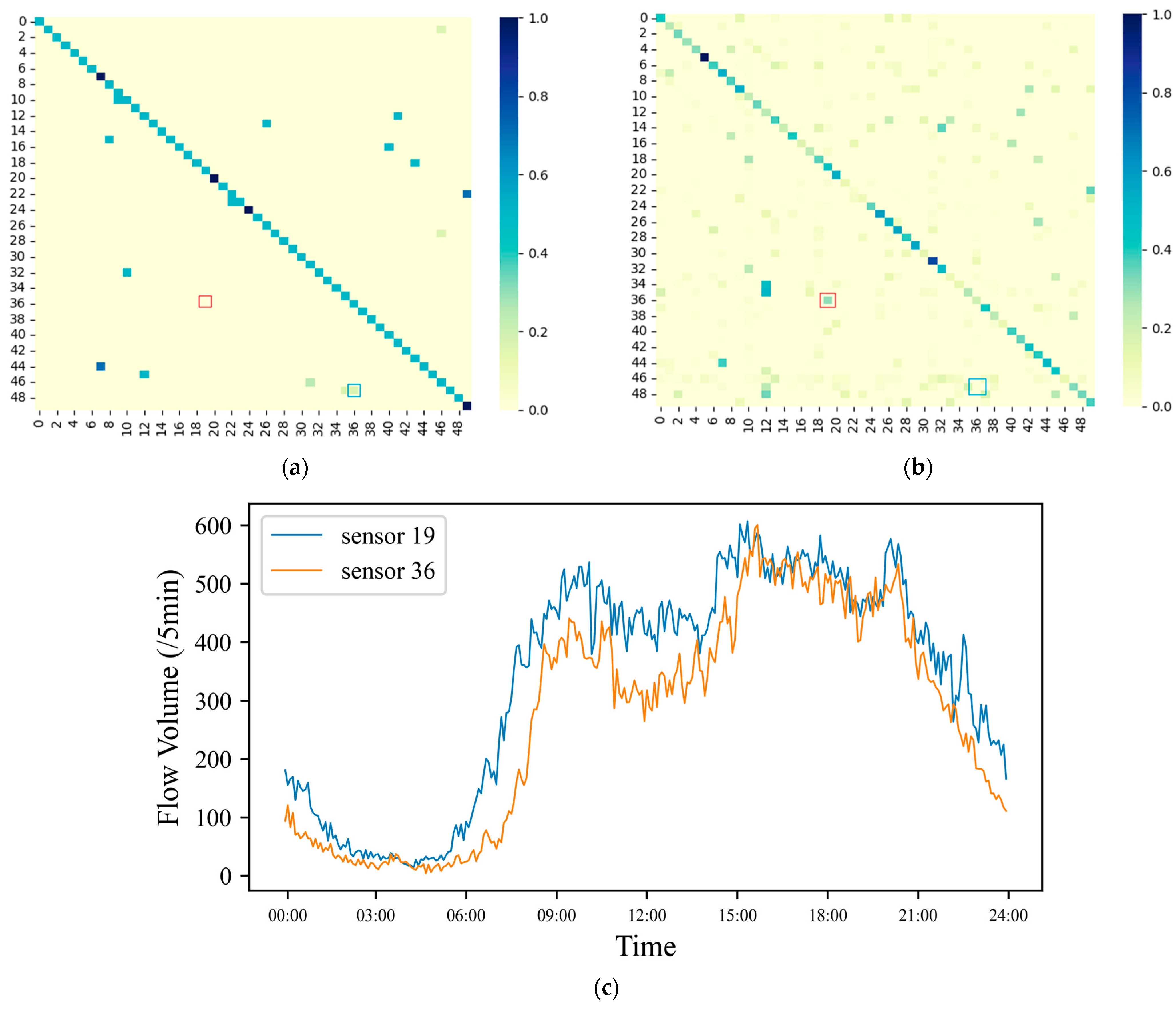
4.7. Research on the Validity of Static Topology Graph

To visualize the effectiveness of the static topology map, we selected the top 50 sensors in the PeMS04 dataset as our research focus. Figure 7a shows the sensor correlation heat map of the adjacency matrix graph, and Figure 7b shows the sensor correlation heat map of the static topology graph. Comparing the two heat maps, it can be seen that the static topology map has been adjusted many times on the basis of the adjacency matrix. Static topology maps learn from predefined mappings, thus preserving some of their basic characteristics. However, unlike the predefined graph, the adaptive graph learns some hidden relationships in the road network structure; for example, static topology weakens the relationship between sensor 36 and sensor 47 and enhances the influence of sensor 19 on sensor 36. In this case, sensor 19 and sensor 36 are not directly connected geographically, but adaptive graph learning reveals a strong hidden correlation between them. We visualized the traffic flow curves of sensor 19 and sensor 36 within a day, and it can be seen from the graph that sensor 19 and sensor 36 have a high spatial correlation with each other. This indicates that the adjacency matrix graph cannot express the true node dependency because two sensors with close geographical locations may not always have strong dependencies, which further indicates that our static topology graph can find the hidden spatial dependencies in the road network.

5. Conclusions

This paper proposes a new traffic flow prediction model called DGSTN. DGSTN introduces a set of adaptive graphs, including static topological graphs that can explore accurate spatial correlations and dynamic information graphs that explore dynamic traffic features. The method mines the features between nodes to characterize genuine traffic node relationships. The model is a spatial-temporal module consisting of multi-scale gated convolution and adaptive spatial attention for exploring accurate spatial-temporal correlations. An empirical study on two traffic datasets shows that DGSTN achieves superior performance. The effectiveness of the components is demonstrated by ablation experiments and visualization of the static topological matrix, which indicate that the model has a very high potential for exploring fundamental spatial-temporal structures. In addition, the graph structure’s high flexibility and extensibility indicate that the model is innovative, useful, and practical. We use multi-headed attention to interact with the graph structure to capture the spatial structure. Although we can capture the relevance from a global graph, developing a more lightweight model is necessary because multi-headed attention uses dot products for computation, something which requires enormous computational effort. In the next step, we can further apply the proposed framework to other spatial-temporal sequence prediction tasks, such as the evolution of social networks, weather, and air quality prediction, etc.

References

1. Wan, S.; Ding, S.; Chen, C. Edge computing enabled video segmentation for real-time traffic monitoring in internet of vehicles. Pattern Recognit. 2022, 121, 108146. [Google Scholar] [CrossRef]
2. Busacca, F.; Grasso, C.; Palazzo, S.; Schembra, G. A smart road side unit in a microeolic box to provide edge computing for vehicular applications. IEEE Trans. Green Commun. Netw. 2022, 7, 194–210. [Google Scholar] [CrossRef]
3. Spandonidis, C.; Giannopoulos, F.; Sedikos, E.; Reppas, D.; Theodoropoulos, P. Development of a MEMS-based IoV system for augmenting road traffic survey. IEEE Trans. Instrum. Meas. 2022, 71, 1–8. [Google Scholar] [CrossRef]
4. Chu, T.; Wang, J.; Codecà, L.; Li, Z. Multi-agent deep reinforcement learning for large-scale traffic signal control. IEEE Trans. Intell. Transp. Syst. 2019, 21, 1086–1095. [Google Scholar] [CrossRef]
5. Feng, J.; Li, Y.; Zhang, C.; Sun, F.; Meng, F.; Guo, A.; Jin, D. Deepmove: Predicting human mobility with attentional recurrent networks. In Proceedings of the 2018 World Wide Web Conference, Lyon, France, 23–27 April 2018; pp. 1459–1468. [Google Scholar] [CrossRef]
6. Gao, Q.; Zhou, F.; Trajcevski, G.; Zhang, K.; Zhong, T.; Zhang, F. Predicting human mobility via variational attention. In Proceedings of the World Wide Web Conference, San Francisco, CA, USA, 13–17 May 2019; pp. 2750–2756. [Google Scholar] [CrossRef]
7. Chen, C.; Petty, K.; Skabardonis, A. Freeway performance measurement system: Mining loop detector data. Transp. Res. Rec. 2001, 1748, 96–102. [Google Scholar] [CrossRef]
8. Williams, B.M.; Hoel, L.A. Modeling and forecasting vehicular traffic flow as a seasonal ARIMA process: Theoretical basis and empirical results. J. Transp. Eng. 2003, 129, 664–672. [Google Scholar] [CrossRef]
9. Jeong, Y.S.; Byon, Y.J.; Castro-Neto, M.M.; Easa, S.M. Supervised weighting-online learning algorithm for short-term traffic flow prediction. IEEE Trans. Intell. Transp. Syst. 2013, 14, 1700–1707. [Google Scholar] [CrossRef]
10. Van Lint, J.W.C.; Van Hinsbergen, C. Short-term traffic and travel time prediction models. Artif. Intell. Appl. Crit. Transp. Issues 2012, 22, 22–41. [Google Scholar]
11. Bildirici, M.; Bayazit, N.G.; Ucan, Y. Modelling oil price with lie algebras and long short-term memory networks. Mathematics 2021, 9, 1708. [Google Scholar] [CrossRef]
12. Ersin, Ö.Ö.; Bildirici, M. Financial Volatility Modeling with the GARCH-MIDAS-LSTM Approach: The Effects of Economic Expectations, Geopolitical Risks and Industrial Production during COVID-19. Mathematics 2023, 11, 1785. [Google Scholar] [CrossRef]
13. Li, Y.; Yu, R.; Shahabi, C. Diffusion convolutional recurrent neural network: Data-driven traffic forecasting. arXiv 2017, arXiv:1707.01926. [Google Scholar] [CrossRef]
14. Seo, Y.; Defferrard, M.; Vandergheynst, P.; Bresson, X. Structured sequence modeling with graph convolutional recurrent networks. In Proceedings of the Neural Information Processing: 25th International Conference, ICONIP 2018, Siem Reap, Cambodia, 13–16 December 2018; pp. 362–373. [Google Scholar] [CrossRef]
15. Yan, S.; Xiong, Y.; Lin, D. Spatial temporal graph convolutional networks for skeleton-based action recognition. In Proceedings of the Thirty-Second AAAI Conference on Artificial Intelligence, New Orleans, LA, USA, 2–7 February 2018. [Google Scholar] [CrossRef]
16. Wu, Z.; Pan, S.; Long, G. Graph wavenet for deep spatial-temporal graph modeling. arXiv 2019, arXiv:1906.00121. [Google Scholar] [CrossRef]
17. Guo, S.; Lin, Y.; Feng, N.; Song, C.; Wan, H. Attention based spatial-temporal graph convolutional networks for traffic flow forecasting. In Proceedings of the AAAI conference on artificial intelligence, Honolulu, HI, USA, 27–28 January 2019; pp. 922–929. [Google Scholar] [CrossRef]
18. Song, C.; Lin, Y.; Guo, S.; Wan, H. Spatial-temporal synchronous graph convolutional networks: A new framework for spatial-temporal network data forecasting. In Proceedings of the AAAI Conference on Artificial Intelligence, New York, NY, USA, 7–12 February 2020; pp. 914–921. [Google Scholar] [CrossRef]
19. Oord, A.; Dieleman, S.; Zen, H. Wavenet: A generative model for raw audio. arXiv 2016, arXiv:1609.03499. [Google Scholar] [CrossRef]
20. Bai, S.; Kolter, J.Z.; Koltun, V. An empirical evaluation of generic convolutional and recurrent networks for sequence modeling. arXiv 2018, arXiv:1803.01271. [Google Scholar] [CrossRef]
21. Yu, F.; Koltun, V. Multi-scale context aggregation by dilated convolutions. arXiv 2015, arXiv:1511.07122. [Google Scholar] [CrossRef]
22. Yu, B.; Yin, H.; Zhu, Z. Spatial-temporal graph convolutional networks: A deep learning framework for traffic forecasting. arXiv 2017, arXiv:1709.04875. [Google Scholar] [CrossRef]
23. Chen, W.; Chen, L.; Xie, Y.; Cao, W.; Gao, Y.; Feng, X. Multi-range attentive bicomponent graph convolutional network for traffic forecasting. In Proceedings of the AAAI Conference on Artificial Intelligence, New York, NY, USA, 7–12 February 2020; pp. 3529–3536. [Google Scholar] [CrossRef]
24. Bai, L.; Yao, L.; Li, C.; Wang, C. Adaptive graph convolutional recurrent network for traffic forecasting. Adv. Neural Inf. Process. Syst. 2020, 33, 17804–17815. [Google Scholar] [CrossRef]
25. Beltagy, I.; Peters, M.E.; Cohan, A. Longformer: The long-document transformer. arXiv 2020, arXiv:2004.05150. [Google Scholar] [CrossRef]
26. Devlin, J.; Chang, M.W.; Lee, K.; Toutanova, K. Bert: Pre-training of deep bidirectional transformers for language understanding. arXiv 2018, arXiv:1810.04805. [Google Scholar] [CrossRef]
27. Arnab, A.; Dehghani, M.; Heigold, G.; Sun, C.; Lučić, M.; Schmid, C. Vivit: A video vision transformer. In Proceedings of the IEEE/CVF Conference on Computer Vision and Pattern Recognition (CVPR), New Orleans, LA, USA, 20–25 June 2021; pp. 6836–6846. [Google Scholar]
28. Bao, H.; Dong, L.; Piao, S.; Wei, F. Beit: Bert pre-training of image transformers. arXiv 2021, arXiv:2106.08254. [Google Scholar] [CrossRef]
29. Zheng, C.; Fan, X.; Wang, C.; Qi, J. Gman: A graph multi-attention network for traffic prediction. In Proceedings of the AAAI Conference on Artificial Intelligence, New York, NY, USA, 7–12 February 2020; pp. 1234–1241. [Google Scholar] [CrossRef]
30. Guo, S.; Lin, Y.; Wan, H. Learning dynamics and heterogeneity of spatial-temporal graph data for traffic forecasting. IEEE Trans. Knowl. Data Eng. 2021, 34, 5415–5428. [Google Scholar] [CrossRef]
31. Xu, M.; Dai, W.; Liu, C.; Gao, X.; Lin, W.; Qi, G.J.; Xiong, H. Spatial-temporal transformer networks for traffic flow forecasting. arXiv 2020, arXiv:2001.02908. [Google Scholar] [CrossRef]
32. Vaswani, A.; Shazeer, N.; Parmar, N.; Uszkoreit, J.; Jones, L.; Gomez, A.N.; Kaiser, Ł.; Polosukhin, I. Attention is all you need. arXiv 2017, arXiv:1706.03762. [Google Scholar] [CrossRef]
33. Shao, Z.; Zhang, Z.; Wei, W.; Wang, F.; Xu, Y.; Cao, X.; Jensen, C.S. Decoupled dynamic spatial-temporal graph neural network for traffic forecasting. arXiv 2022, arXiv:2206.09112. [Google Scholar] [CrossRef]
34. Shin, Y.; Yoon, Y. Pgcn: Progressive graph convolutional networks for spatial-temporal traffic forecasting. arXiv 2022, arXiv:2202.08982. [Google Scholar] [CrossRef]
Figure 1. Findings on traffic prediction; (a) Spatial dependence changes dynamically over time. (b) Hidden spatial dependencies.
Mathematics 11 02528 g001
Figure 2. The framework of Dynamic Graph Spatial−Temporal Neural Network (DGSTN). (a) DGSTN architecture; (b) ST block; (c) Adaptive graph.
Mathematics 11 02528 g002
Figure 3. Different types of attention. (a) Fully connected spatial attention; (b) Adaptive spatial attention. The numbers in the upper panels in (a,b) represent the geographic nodes where they are located, and the figures in the lower panels represent the corresponding spatial attention matrices. Among them, green represents the self-connection of nodes, blue represents fully connected spatial attention, indicating that each node is related to each other, and yellow represents adaptive spatial attention, indicating that each node is adaptively associated.
Mathematics 11 02528 g003
Figure 4. Performance comparison of the tested models at each horizon on PeMS04 and PeMS08 dataset for traffic flow prediction, where one horizon denotes 5 min.
Mathematics 11 02528 g004
Figure 5. Visualization on the PeMS08 dataset. (a) Visualization of node 7 of the PeMS08 dataset; (b) Visualization of node 157 of the PeMS08 dataset.
Mathematics 11 02528 g005aMathematics 11 02528 g005b
Figure 6. Ablation study on the PeMS04 dataset.
Mathematics 11 02528 g006
Figure 7. Analyzing the effectiveness of static topology graph research on the PeMS04 dataset. (a) Predefined adjacency matrix heat map; (b) Heat map of the graph matrix obtained by static topology graph; (c) One-day traffic flow on sensors 19 and 36.
Mathematics 11 02528 g007