Dual Space Latent Representation Learning for Image Representation

Abstract

Semi-supervised non-negative matrix factorization (NMF) has achieved successful results due to the significant ability of image recognition by a small quantity of labeled information. However, there still exist problems to be solved such as the interconnection information not being fully explored and the inevitable mixed noise in the data, which deteriorates the performance of these methods. To circumvent this problem, we propose a novel semi-supervised method named DLRGNMF. Firstly, dual latent space is characterized by the affinity matrix to explicitly reflect the interrelationship between data instances and feature variables, which can exploit the global interconnection information in dual space and reduce the adverse impacts caused by noise and redundant information. Secondly, we embed the manifold regularization mechanism in the dual graph to steadily retain the local manifold structure of dual space. Moreover, the sparsity and the biorthogonal condition are integrated to constrain matrix factorization, which can greatly improve the algorithm’s accuracy and robustness. Lastly, an effective alternating iterative updating method is proposed, and the model is optimized. Empirical evaluation on nine benchmark datasets demonstrates that DLRGNMF is more effective than competitive methods.

1. Introduction

Dimensionality reduction for image representation is a fundamental task in machine learning. Dimensionality reduction can not only shorten computation time and reduce storage space, but also find out latent and discriminative features by removing the noise and irrelevant features. Over the past decade, many dimensionality reduction methods have been presented such as locally linear embedding (LLE) [1], non-negative matrix factorization (NMF) [2,3], feature selection (FS) [4], and principal component analysis (PCA) [5]. In particular, due to its excellent low-dimensional learning ability, NMF has attracted a lot of attention and been successfully applied to image analysis [6], text classification [7], face recognition [8], and biometrics [9].

NMF is expressed as low-dimensional representations of high-dimensional data [10]. Since there is a constraint that these low-dimensional matrices are negative in NMF, the part-of-whole interpretation can be guaranteed and is consistent with human perception [11]. However, there are some limitations to NMF. Firstly, NMF ignores local data structure [12] since the data with a non-Gaussian distribution do not satisfy the constraint condition that the samples are only restricted to the number of classes in NMF. Secondly, recent studies show that sparse representation can improve the robustness and recognition of the algorithm to some extent, whereas NMF is not able to generate sparse representation. Furthermore, NMF is an unsupervised method that fails to investigate partial label information. However, in the real world, a small amount of label information is easily available. Lastly, in NMF there is an assumption that data instances are distributed and independent, which results in ignoring the interconnection of data instances in the real world. Nonetheless, whether data instances come from homologous sources or heterogeneous sources, there will be some interconnection between them [13], as well as between feature variables. For data instances, each data instance exhibits a certain degree of correlation that stronger correlation among samples may occur in the same class and weaker correlation among samples may exist in different classes. For example, as shown in Figure 1, Figure 1a–c represent three kinds of faces belonging to three different classes in the ORL dataset [14]. At first glance, there exists a common object, i.e., eyeglasses, in Figure 1a,b, whereas there is no common object in Figure 1b,c. Despite these groups of images belonging to different classes, the eyeglasses feature exhibits a moderate correlation to some extent within these two categories in Figure 1a,b. However, the correlation in the eyeglasses feature between Figure 1b and Figure 1c is low. By leveraging NMF to learn these interconnected relationships as prior knowledge and performing matrix factorization, the resulting low-dimensional representation will produce satisfactory outcomes within the constraints of this information. Furthermore, due to the diversity of samples, as in Figure 1a, the eyes are unable to act as a dominant feature for classification because the glasses play an important role to some extent. Hence, the interconnection of the eyes and the glasses can successfully distinguish the faces in Figure 1a,c.

To solve the above problems in NMF, various NMF variants have been proposed. To establish local data structure, i.e., the first limitation of NMF, Huang et al. [15] and Cai et al. [16] presented new NMF variants with a neighborhood graph to enable a compact representation of similar data points in the data space consistent with coefficient vectors. Different from the above two methods, Liu et al. [17] introduced the local coordinate constraint, which can enable the base vectors close to the samples. To sufficiently exploit the local manifold structure in data space and feature space, Shang et al. [18] constructed a dual graph model by encoding geometric information. Since the sparsity of NMF is not enough, Hoyer [19] introduced the sparsity of the coefficient matrix into NMF to explore parts-based representations and control the degree of sparseness explicitly. On the basis of the method in [19], Meng et al. [20] obtained the sparse basis matrix by imposing the ℓ_2,1-norm while considering the local manifold structure in the dual space. To utilize partial label information, some researchers [21,22,23] constructed a stronger constraint and embed it into NMF to perform semi-supervised NMF. Different from previous semi-supervised NMF algorithms that shared the same coordinates for data points with the same labels, an additional constraint in the new representation was imposed to distribute the samples of the same class on the same axis, which could improve the robustness of clustering [24]. Integrating the merits of dual graph regularization, sparse regression, and semi-supervised, Meng et al. [25] imposed biorthogonal constraints to perform a semi-supervised non-negative matrix factorization. Thus, a unique basis vector corresponded to each image, which efficiently improved the discrimination ability of clusters and the exclusion between different classes. In fact, the interconnection information in NMF has not been adequately investigated. Recently, latent representation has been applied in the data space [26,27] or feature space [28] due to its good performance in exploiting the interconnection information. However, how to employ a fraction of label information to associate a small number of data instances and feature variables in latent representation space remains a challenging problem.

In summary, there are still some problems to be solved in NMF. These methods related to NMF are listed in terms of their characteristics in

Table 1. Summary of the state-of-the-art NMF variants.

Methods	Semi-Supervised	Sparse Representation	Local Data Structure	Interconnection Information
NMF with sparseness constraints (2004) [19]	√	×	×	×
Constrained NMF (CNMF) (2012) [21]	√	×	×	×
Graph regularized NMF (GNMF) (2011) [16]	×	×	√	×
Graph dual regularization NMF (DNMF) (2012) [18]	×	×	√	×
Robust manifold NMF (RMNMF) (2014) [15]	×	×	√	×
Local coordinate concept factorization (LCF) (2014) [17]	×	√	√	×
Discriminative NMF (2016) [24]	√	×	×	×
Adaptive dual-graph regularized CF with FS (ADGCFFS) (2017) [29]	×	×	√	×
NMF with adaptive neighbors (NMFAN) (2017) [30]	×	×	√	×
Dual-graph sparse NMF (DSNMF) (2018) [20]	×	√	√	×
Dual-regularized multi-view NMF (DMvNM) (2018) [31]	×	×	√	×
Dual-graph regularized NMF with sparse and orthogonal constraints (SODNMF) (2018) [25]	√	√	√	×
Correntropy-based semi-supervised NMF (CSNMF) (2021) [22]	×	×	√	×
Discriminative semi-supervised NMF (DSSNMF) (2021) [32]	√	×	×	×
Feature weighted NMF (FNMF) (2021) [12]	×	×	√	×
Entropy weighted robust NMF (EWRNMF) (2022) [33]	×	×	×	×
Semi-supervised graph regularized NMF with local coordinate (SGLNMF) (2022) [34]	√	√	√	×
Self-supervised semi-supervised NMF (S4NMF) (2023) [35]	√	×	×	×
Semi-supervised NMF with adaptive neighbors and block-diagonal (ABNMTF) (2023) [36]	√	×	√	×
DLRGNMF (this study)	√	√	√	√

to enhance the comparative of overcoming the limitations of NMF.

Inspired by latent representation, we propose a novel method named semi-supervised NMF via dual space latent representation learning and dual graph regularization (DLRGNMF) to alleviate the above issues. The main contributions of our work are as follows:

(1)

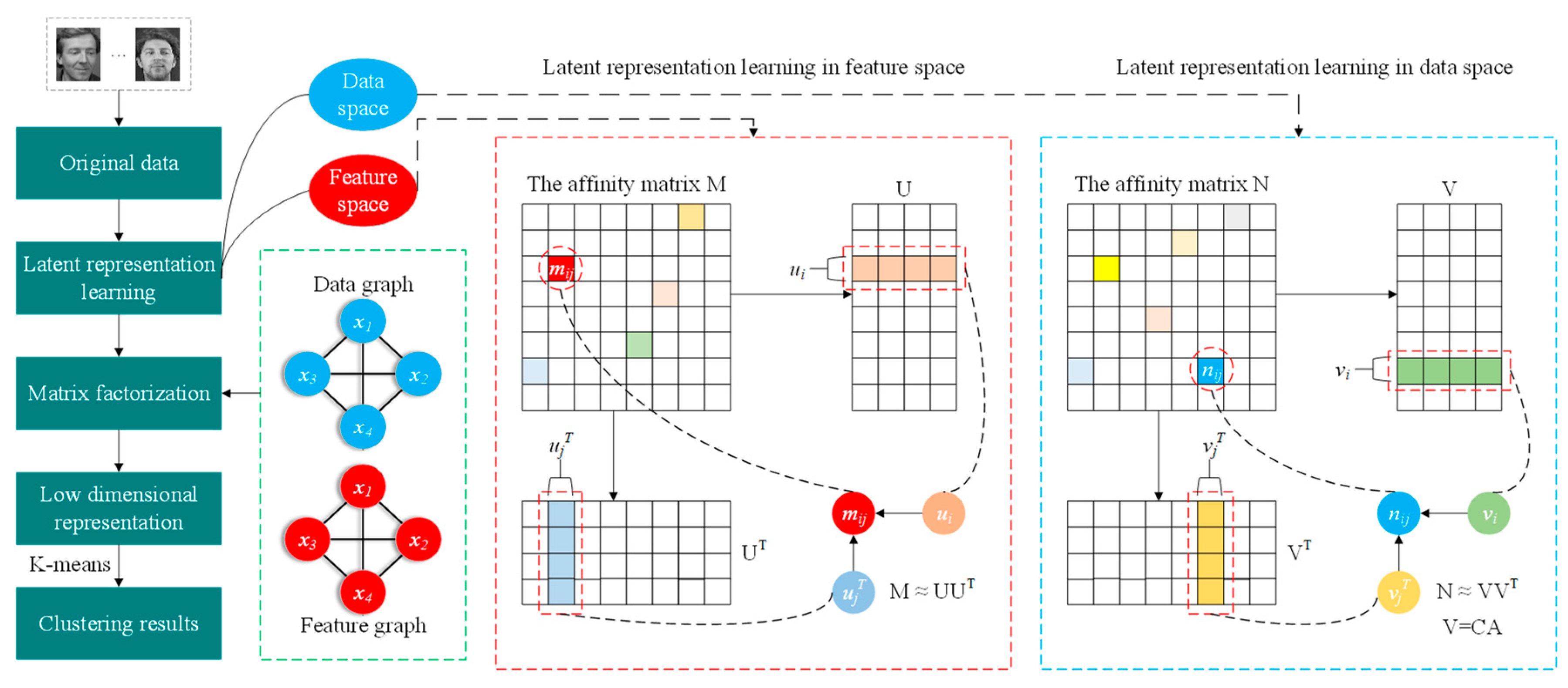
The dual latent representation mechanism is embedded into the semi-supervised NMF framework by the affinity matrix to explicitly exploit global interconnection information in dual space, which can reduce the adverse impacts caused by noise.

(2)

To steadily describe local data structures, the dual graph is introduced into latent representation learning to further fully investigate the coherent information structure in dual space.

(3)

To achieve a sparse representation of matrix factorization, the ℓ_2,1-norm is incorporated into the basis matrix $U$ in the proposed framework, which can simplify the measurement process and improve the clustering performance.

In conclusion, our proposed method can overcome the limitations of NMF to some extent. In real applicated fields our proposed method can be applied to image analysis, text classification, attribute community detection, face recognition, and recommender system.

This paper is constructed as follows: we review the related studies in Section 2; Section 3 illustrates the DLRGNMF algorithm, gives the iterative update rules, and provides a detailed analysis of convergence analysis; Section 4 evaluates DLRGNMF in terms of clustering analysis and ablation experiments; lastly, we summarize the conclusion in Section 5.

2. Related Work

In this section, we briefly review the algorithms related to our work.

2.1. CNMF

Studies show that, in semi-supervised algorithms, a small fraction of label information can improve the accuracy of learning [37,38]. As an extension of NMF, CNMF [21] incorporates the label information to improve the discriminating power, thus attaching label information to NMF as hard constraints. The objective function of CNMF is formulated as follows:

$$\begin{gathered} O_{CNMF}=\Vert X-U{Z}^T{A}^T{\Vert }_F^2, \\ s.t. U\ge 0, Z\ge 0, \end{gathered}$$

(1)

where $Z$ is a label constraint matrix and $A$ is a label auxiliary matrix. This strategy by constraint of $Z$ can require the samples with the same label to be consistent to coordinate in the mapping space. Liu et al. [21] gave proof of the update iteration rule for CNMF and its convergence. CNMF integrates the merits of NMF and a semi-supervised mechanism to improve its discriminating power.

2.2. DNMF

Motivated by manifold learning theory, Shang et al. proposed DNMF [18], which constructs neighborhood graphs according to the observation data on the structure of data and feature manifold. The objective function of DNMF is formulated as follows:

$$\begin{gathered} O_{DNMF}=\Vert X-U{V}^T{\Vert }_F^2+\lambda Tr\left(V^T{L}_{Z}V\right)+\mu Tr\left(U^T{L}_{U}U\right), \\ s.t. U\ge 0, V\ge 0, \end{gathered}$$

(2)

where $\lambda$ and $\mu$ are graph regularization parameters. DNMF integrates the virtues of dual graph regularization to perform matrix factorization to further enhance its learning ability.

2.3. SODNMF

Inspired by CNMF and DNMF, Meng et al. [25] designed SODNMF. The geometric manifold information can be effectively modeled by adopting dual graph regularization constraints to NMF. Furthermore, the sparse constraint is also embedded to guarantee the sparsity. The objective function of SODNMF is expressed as

$$\begin{gathered} O_{SODNMF}=\Vert X-PR{A}^T{C}^T{\Vert }_F^2+\alpha \left[Tr\left(P^T{L}^{P}P\right)+Tr\left(A^T{C}^T{L}^{S}CA\right)\right]+\theta \Vert P{\Vert }_{\frac{2,1}{2}}^{\frac{1}{2}}, \\ s.t. P^{T}P=I,A^T{C}^{T}CA=I, \end{gathered}$$

(3)

where $\alpha$ is the regularization parameter, and $\theta$ is the sparse constraint parameter. The two terms associated with $\alpha$ are dual graph regularization terms, and the term is controlled by $\theta$ is a sparse constraint.

2.4. LRLMR

Traditional unsupervised feature selection methods ignore the interrelationship between data instances. For this reason, Tang et al. presented unsupervised feature selection via latent representation learning and manifold regularization (LRLMR) [26], integrating latent representation learning into the local manifold information to perform feature selection, which can explore the global interrelationship of data space by constructing an affinity matrix. LRLMR formulates the objective function as follows:

$$\begin{gathered} O_{LRLMR}=\Vert XW-V{\Vert }_F^2+\alpha \Vert W{\Vert }_{2,1}+\beta \Vert A-V{V}^T{\Vert }_F^2+\gamma Tr\left(W^T{X}^{T}LXW\right), \\ s.t. V\ge 0, \end{gathered}$$

(4)

where $\alpha$ is the sparse constraint parameter, $\beta$ is the latent representation learning parameter, and $\gamma$ is the manifold regularization parameter. LRLMR learns the latent representation matrix $V$ into a pseudo-label matrix to yield the clustering index and further reduce noise.

2.5. Latent Representation

Latent representations of data have yielded promising results and attracted considerable attention in machine learning tasks. In the real world, the purpose of latent representations is to establish the link information through DMvNM [31], DSSNMF [32], ADGCF_FS [29], symmetric NMF [39], etc. Generally, latent representation constructs an affinity matrix $P\in R^{n\times n}$ to describe the interconnection information between samples by decomposing $P$ through a symmetric NMF, which is represented as follows:

$$R=\Vert P-V{V}^T{\Vert }_F^2,$$

(5)

where $V\in R^{n\times k}$ is the low-dimensional representation by mapping to the new representation space, while $k$ and $n$ denote latent factors and the number of samples, respectively. The affinity matrix $P$ indicates the global interconnection information between samples. However, interconnection information exists not only in data instances but also between features [28]. Figure 2 illustrates Pearson correlation coefficients between data instances and feature variables of the Soybean dataset to demonstrate the interconnection relationship. It can be clearly observed that, in Figure 2a,b, the absolute values of Pearson correlation coefficients are higher than 0.3 in most cases, especially in Figure 2a, which implies that there is strongly correlated interconnection information between data instances and correlated interconnection information feature variables; that is, interconnection information exists in dual space.

3. Proposed Method

Inspired by the theory in the literature [28,39], we propose a novel model dual space based on latent representation learning named DLRGNMF, whose pipeline is visualized in Figure 3.

3.1. Dual Space Latent Representation Learning and Dual Graph Regularization

Conventional non-negative matrix factorization algorithms always assume that the data are independently and uniformly distributed by default. However, this kind of distribution is not ideal in actual application. Since noise is generated by various factors, the data instances derived from homology or heterogeneity are often interdependent [13,40]. Therefore, it is significant to exploit the intrinsic data structure and feature structure through link information. Some dimensionality reduction algorithms [26,27,41] implemented this idea by virtue of latent representation learning and achieved excellent results. Inspired by these algorithms, we embed dual space latent representation learning into the semi-supervised learning of NMF by mapping the original data to learn the dual latent space of matrix factorization. Thus, the interconnection of information is investigated in mining dual space simultaneously to reduce the influence of the noise, and to improve the robustness of matrix factorization.

To perform matrix factorization in the learned dual latent space, we construct the objective function of the dual space latent representation learning as follows:

$$R_1=\Vert M-CA{A}^T{C}^T{\Vert }_F^2+\Vert N-U{U}^T{\Vert }_F^2,$$

(6)

where $A\in {\mathcal{R}}^{\left(n+c-l\right)\times c}$ is label auxiliary matrix, $U\in {\mathcal{R}}^{m\times c}$ is the basis matrix, $C\in {\mathcal{R}}^{n\times \left(n+c-l\right)}$ is the label constraint matrix [21], $n$ is the number of samples, $l$ is the number of labeled data points, and $c$ is the number of categories. The first term is to the latent representation of the data space by constructing an affinity matrix $M\in {\mathcal{R}}^{n\times n}$ in the data space, which can reflect inherent information between instances. The unlabeled dataset is defined by $X=\left[x_1,x_2,\dots ,x_n\right]\in R^{m\times n}$, where $m$ is the feature dimension of the sample. The affinity matrix $M$ is defined as follows:

$$M_{ij}=exp\left(-\frac{\Vert x_i-x_j{\Vert }^2}{2{\sigma }^2}\right), i,j=1,2,\dots ,n.$$

(7)

The second term in Equation (6) is constructed by an affinity matrix $N\in {\mathcal{R}}^{m\times m}$ to learn the feature latent space and investigate inherent information between features. The affinity matrix $N$ is defined as follows:

$$N_{ij}=exp\left(-\frac{\Vert y_i-y_j{\Vert }^2}{2{\sigma }^2}\right), i,j=1,2,\dots ,m,$$

(8)

where $x_i$, $y_i$, and $\sigma$ denote the $i$-th sample, the $i$-th feature of the data matrix $X$, and a Gaussian bandwidth parameter, respectively, with $0<M_{ij}\le 1,0<N_{ij}\le 1$. $M_{ij}$ and $N_{ij}$ represent the interrelation between the $i$-th and $j$-th data instances and the interrelation between the $i$-th and $j$-th feature vectors, respectively. Therefore, $M_{ij}$ and $N_{ij}$ describe the global interconnection information in the dual space and learn this information through the situation of the symmetric NMF; therefore, the corresponding low-dimensional representation can be accomplished by matrix factorization under the constraints of this information.

With the development of graph theory and spectral theory, graph regularization has been successfully applied to NMF. In Equation (6), we introduce latent representation learning which maps the raw data into the dual latent space, thus constructing a Laplacian regularization term for dual graph [18], which is represented as follows:

$$R_2=Tr\left(U^T{L}^{N}U\right)+Tr\left(A^T{C}^T{L}^{M}CA\right),$$

(9)

where $L^M\in {\mathcal{R}}^{n\times n}$ is the Laplacian matrix of the data space and $L^M=D^M-S^M$, $D^M$ satisfies ${\left[D^M\right]}_{ii}={{\displaystyle \sum }}_j{\left[S^M\right]}_{ij}$, and $S^M$ is the similarity matrix constructed by the $k$-neighborhood graph $M_k\left(x_i\right)$ as follows:

$${\left[S^M\right]}_{ij}=\left\{\begin{array}{c}{M}_{ij}, if{x}_j\in M_k\left(x_i\right)\hfill \\ \\ 0, otherwise\hfill \end{array}\right. i,j=1,2,3,\dots ,n.$$

(10)

Similarly, the Laplacian matrix of the feature space is denoted as $L^N\in {\mathcal{R}}^{m\times m}$ and $L^N=D^N-S^N$, $D^N$ satisfies ${\left[D^N\right]}_{ii}={{\displaystyle \sum }}_j{\left[S^N\right]}_{ij}$, and $S^N$ is the similarity matrix, constructed as follows:

$${\left[S^N\right]}_{ij}=\left\{\begin{array}{c}{N}_{ij}, if{y}_j\in N_k\left(y_i\right)\hfill \\ \\ 0, otherwise\hfill \end{array}\right. i,j=1,2,3,\dots ,m,$$

(11)

where $N_k\left(y_i\right)$ is a $k$-neighborhood graph.

3.2. Objective Function

First, we construct the objective function for the semi-supervised NMF as follows [25]:

$$\begin{gathered} \left(U^{*},R^{*},C^{*},A^{*}\right)=arg min \Vert X-UR{A}^T{C}^T{\Vert }_F^2, \\ s.t.U^{T}U=I,A^T{C}^{T}CA=I. \end{gathered}$$

(12)

We incorporate biorthogonal constraints in the semi-supervised NMF, which possesses the robust ability to classify basic and coefficient vectors simultaneously to improve cluster performance. Since biorthogonal constraints are strong constraints, diagonal scaling matrix $R$ can be utilized to avoid the problem of generating unreliable solutions. To simplify the calculation, the ℓ_2,1-norm is introduced to the basis matrix $U$, and the novel objective function is expressed as follows:

$$\begin{gathered} \left(U^{*},R^{*},C^{*},A^{*}\right)=arg min \Vert X-UR{A}^T{C}^T{\Vert }_F^2+\theta \Vert U{\Vert }_{2,1}. \\ s.t. U^{T}U=I, A^T{C}^{T}CA=I. \end{gathered}$$

(13)

where $\theta$ is the sparse constraint parameter, and $\theta >0$ controls the sparsity of the model.

DLRGNMF integrates dual space latent representation learning and dual graph regularization into a semi-supervised NMF framework. Combining Equations (6), (9), and (13), the final objective function of DLRGNMF is transformed into the following:

$$\begin{gathered} \left(U^{*},R^{*},C^{*},A^{*}\right)=arg min \Vert X-UR{A}^T{C}^T{\Vert }_F^2+\alpha \left[Tr\left(U^T{L}^{N}U\right)+Tr\left(A^T{C}^T{L}^{M}CA\right)\right] \\ +\frac{\gamma }{2}\left[\Vert M-CA{A}^T{C}^T{\Vert }_F^2+\Vert N-U{U}^T{\Vert }_F^2\right]+\theta \Vert U{\Vert }_{2,1}, \end{gathered}$$

(14)

$$s.t. U^{T}U=I, A^T{C}^{T}CA=I,$$

where $\alpha$ and $\gamma$ are the dual graph regularization parameter and the dual space parameter, respectively, and $\alpha$, $\gamma$, $\theta >0$, which can balance the weight of the above terms.

3.3. Optimization

In this subsection, the optimization principle of DLRGNMF is illustrated. Since the objective function in Equation (14) is simultaneously nonconvex with $U$, $R$, $C$, and $A$, it is challenging to solve. To solve the objective function in Equation (14), the objective function with a single variable is convex and can be optimized by the alternate iterative method. Thus, the entire optimization problem can be decomposed into four subproblems. By optimizing this objective function of DLRGNMF, the parameter $\beta$ is expressed as the biorthogonal parameter to restrict the biorthogonal term and $\beta >0$. Therefore, the Lagrange Equation (15) is constructed as follows:

$$\begin{gathered} L\left(U,R,C,A\right)=\Vert X-UR{A}^T{C}^T{\Vert }_F^2+\alpha Tr\left(U^T{L}^{N}U\right)+\alpha Tr\left(A^T{C}^T{L}^{M}CA\right)+\beta Tr\left(U^{T}U-I\right)+\beta Tr\left(A^T{C}^{T}CA-I\right) \\ +\frac{\gamma }{2}\Vert M-CA{A}^T{C}^T{\Vert }_F^2+\frac{\gamma }{2}\Vert N-U{U}^T{\Vert }_F^2+\theta Tr\left(U^{T}QU\right), \end{gathered}$$

(15)

where $Q\in {\mathcal{R}}^{m\times m}$ is a diagonal matrix, and we can calculate the $i$-th diagonal element $q_{ii}$ of $Q$ as follows:

$$q_{ii}=\frac{1}{2\Vert U_i{\Vert }_2}.$$

(16)

To avoid overflow, we introduce a small constant $\epsilon$, and Equation (16) can be represented as

$$q_{ii}=\frac{1}{2\max (\Vert U_i{\Vert }_2,\epsilon )}.$$

(17)

In order to optimize $U$, $R$, $C$, and $A$, the partial derivatives of the Lagrange function in Equation (15) are formulated, yielding

$$\frac{\partial L}{\partial U}=-2XCA{R}^T+2UR{A}^T{C}^{T}CA{R}^T+2\alpha L^{N}U+2\beta U+2\theta QU-2\gamma NU+2\gamma U{U}^{T}U,$$

(18)

$$\frac{\partial L}{\partial R}=-2U^{T}XCA+2U^{T}UR{A}^T{C}^{T}CA,$$

(19)

$$\frac{\partial L}{\partial A}=-2C^T{X}^{T}UR+2C^{T}CA{R}^T{U}^{T}UR+2\alpha C^T{L}^{M}CA+2\beta C^{T}CA-2\gamma C^{T}MCA+2\gamma C^{T}CA{A}^T{C}^{T}CA,$$

(20)

$$\frac{\partial L}{\partial C}=-2X^{T}UR{A}^T+2CA{R}^T{U}^{T}UR{A}^T+2\alpha L^{M}CA{A}^T+2\beta CA{A}^T-2\gamma MCA{A}^T+2\gamma CA{A}^T{C}^{T}CA{A}^T.$$

(21)

Then, according to the KKT condition [42], the iterative update equations for $U$, $R$, $C$, and $A$ are written as follows:

$$u_{ij}\leftarrow u_{ij}\frac{{\left[XCA{R}^T+\alpha W^{N}U+\gamma NU\right]}_{ij}}{{\left[UR{A}^T{C}^{T}CA{R}^T+\alpha D^{N}U+\beta U+\theta QU+\gamma U{U}^{T}U\right]}_{ij}},$$

(22)

$$r_{ij}\leftarrow r_{ij}\frac{{\left[U^{T}XCA\right]}_{ij}}{{\left[U^{T}UR{A}^T{C}^{T}CA\right]}_{ij}},$$

(23)

$$a_{ij}\leftarrow a_{ij}\frac{{\left[C^T{X}^{T}UR+\alpha C^T{W}^{M}CA+\gamma C^{T}MCA\right]}_{ij}}{{\left[C^{T}CA{R}^T{U}^{T}UR+\alpha C^T{D}^{M}CA+\beta C^{T}CA+\gamma C^{T}CA{A}^T{C}^{T}CA\right]}_{ij}},$$

(24)

$$c_{ij}\leftarrow c_{ij}\frac{{\left[X^{T}UR{A}^T+\alpha W^{M}CA{A}^T+\gamma MCA{A}^T\right]}_{ij}}{{\left[CA{R}^T{U}^{T}UR{A}^T+\alpha D^{M}CA{A}^T+\beta CA{A}^T+\gamma CA{A}^T{C}^{T}CA{A}^T\right]}_{ij}}.$$

(25)

With the above analysis, the procedure of DLRGNMF is summarized in

Table 2. DLRGNMF algorithm steps.

Algorithm 1 The optimization process of DLRGNMF
1: Input: Data matrix $\mathrm{X}\in {\mathcal{R}}^{\mathrm{m}\times \mathrm{n}}$, class number of samples c, neighborhood size k, balance parameters α, β, θ and γ, the maximum number of iterations $NIter$, and the ratio of training samples $per$.
2: Initialization: Normalize the data matrix X, generate U, R, and A, and pick up per% as the label information from the original data to construct matrix C, iteration time t = 0;
3: Construct the dual space latent representation learning;
4: Construct the dual-graph regularized model;
5: while not converged do 6:    Update U using Equation (22); 7:    Update R using Equation (23); 8:    Update A using Equation (24); 9:    Update C using Equation (25); 10:     Update Q using Equation (17); 11:     Update t by: t = t + 1, t ≤ NIter; 12: end while
13: Output: The label constraint matrix C, the basis matrix U, the diagonal scaling matrix R, and the label auxiliary matrix A.

.

3.4. Convergence Analysis

In this section, we prove the convergence of DLRGNMF by demonstrating that under the update rules in Equations (22)–(25), the objective function in Equation (14) is monotonically decreasing.

First, we need to introduce a theorem [43], which theoretically guarantees the convergence of DLRGNMF.

Definition 1. 

If there is a function $G\left(x, x\prime \right)$ such that $F\left(x\right)$ satisfies

$$G\left(x,x^{\prime }\right)\ge F\left(x\right),G\left(x,x\right)=F\left(x\right),$$

(26)

$F$ is a nonincreasing function when the updating formula is written as

$$x^{\left(t+1\right)}=\arg \begin{array}{c}min\\ x\end{array}G\left(x,x^{\left(t\right)}\right),$$

(27)

where $G\left(x,x\prime \right)$ is an auxiliary function of $F\left(x\right)$.

Proof. 

$$F\left(x^{\left(t+1\right)}\right)\le G\left(x^{\left(t+1\right)},x^{\left(t\right)}\right)\le G\left(x^{\left(t\right)},x^{\left(t\right)}\right)=F\left(x^{\left(t\right)}\right).$$

(28)

If the objective function is proved to be monotonic, it is retained to contain the $U$ term and transformed into

$$F\left(U\right)=\Vert X-UR{A}^T{C}^T{\Vert }_F^2+\alpha Tr\left(U^T{L}^{N}U\right)+\beta Tr\left(U^{T}U-I\right)+\frac{\gamma }{2}\Vert N-U{U}^T{\Vert }_F^2+\theta Tr\left(U^{T}QU\right).$$

(29)

We can get the partial derivatives of $F\left(U\right)$ in the first order and second order with respect to

$$F_{ij}^{\prime }=-2XCA{R}^T+2UR{A}^T{C}^{T}CA{R}^T+2\alpha L^{N}U+2\beta U+2\theta QU-2\gamma NU+2\gamma U{U}^{T}U,$$

(30)

$$F_{ij}^{″}=2{\left[R{A}^T{C}^{T}CA{R}^T\right]}_{jj}+2{\left[\alpha L^N\right]}_{ii}+2{\left[\beta I\right]}_{ii}+2{\left[\theta Q\right]}_{ii}-2{\left[\gamma N\right]}_{ii}+2{\left[\gamma U{U}^T\right]}_{ii}.$$

(31)

□

Lemma 1. 

$$\begin{gathered} G\left(U_{ij},U_{ij}^{\left(t\right)}\right)=F_{ij}\left(U_{ij}^{\left(t\right)}\right)+F_{ij}^{\prime }\left(U_{ij}^{\left(t\right)}\right)\left(U_{ij}-U_{ij}^{\left(t\right)}\right) \\ +\frac{{\left[UR{A}^T{C}^{T}CA{R}^T+\alpha D^{N}U+\beta U+\theta QU+\gamma U{U}^{T}U\right]}_{ij}}{U_{ij}^{\left(t\right)}}{\left(U_{ij}-U_{ij}^{\left(t\right)}\right)}^2, \end{gathered}$$

(32)

where $G\left(U_{ij},U_{ij}^{\left(t\right)}\right)$ is the auxiliary function of $F_{ij}$.

Proof. 

The Taylor series expansion of $F_{ij}\left(U_{ij}\right)$ is

$$\begin{gathered} F_{ij}\left(U_{ij}\right)=F_{ij}\left(U_{ij}^{\left(t\right)}\right)+F_{ij}^{\prime }\left(U_{ij}^{\left(t\right)}\right)\left(U_{ij}-U_{ij}^{\left(t\right)}\right) \\ +\left\{{\left[R{A}^T{C}^{T}CA{R}^T\right]}_{jj}+{\left[\alpha L^N\right]}_{ii}+{\left[\beta I\right]}_{ii}+{\left[\theta Q\right]}_{ii}-{\left[\gamma N\right]}_{ii}+{\left[\gamma U{U}^T\right]}_{ii}\right\}{\left(U_{ij}-U_{ij}^{\left(t\right)}\right)}^2. \end{gathered}$$

(33)

$G\left(U_{ij},U_{ij}^{\left(t\right)}\right)\ge F_{ij}\left(U_{ij}\right)$ is equivalent to

$$\begin{gathered} \frac{{\left[UR{A}^T{C}^{T}CA{R}^T+\alpha D^{N}U+\beta U+\theta QU+\gamma U{U}^{T}U\right]}_{ij}}{U_{ij}^{\left(t\right)}} \\ \ge {\left[R{A}^T{C}^{T}CA{R}^T\right]}_{jj}+{\left[\alpha L^N\right]}_{ii}+{\left[\beta I\right]}_{ii}+{\left[\theta Q\right]}_{ii}-{\left[\gamma N\right]}_{ii}+{\left[\gamma U{U}^T\right]}_{ii}. \end{gathered}$$

(34)

Since,

$$\left\{\begin{array}{c}{\left[UR{A}^T{C}^{T}CA{R}^T\right]}_{ij}={{\displaystyle \sum }}_k{U}_{ik}^{\left(t\right)}{\left[R{A}^T{C}^{T}CA{R}^T\right]}_{kj}\ge {\left[R{A}^T{C}^{T}CA{R}^T\right]}_{ii}{U}_{ij}^{\left(t\right)}\\ \alpha {\left[D^{N}U\right]}_{ij}=\alpha {{\displaystyle \sum }}_k{\left[D^U\right]}_{ik}{U}_{kj}^{\left(t\right)}\ge \alpha {\left[L^N\right]}_{ii}{U}_{ij}^{\left(t\right)}\\ {\left[\beta U+\theta QU\right]}_{ij}={{\displaystyle \sum }}_k{\left[\beta I+\theta Q\right]}_{ik}{U}_{kj}^{\left(t\right)}\ge \alpha {\left[\beta I+\theta Q\right]}_{ii}{U}_{ij}^{\left(t\right)}\\ \gamma {\left[U{U}^{T}U\right]}_{ij}=\gamma {{\displaystyle \sum }}_k{\left[U{U}^T\right]}_{ik}{U}_{kj}^{\left(t\right)}\ge \gamma {\left[U{U}^T\right]}_{ii}{U}_{ij}^{\left(t\right)}\end{array},\right.$$

(35)

we get $G\left(U_{ij},U_{ij}^{\left(t\right)}\right)\ge F_{ij}\left(U_{ij}\right)$. □

Next, we prove that according to the iterative update rule in Equation (22) $F_{ij}$ is monotonically decreasing.

Substituting Equation (32) $G\left(U_{ij},U_{ij}^{\left(t\right)}\right)$ into Lemma 1 with $x^{\left(t+1\right)}=\arg \begin{array}{c}min\\ x\end{array}G\left(x,x^{\left(t\right)}\right)$,

$$\begin{gathered} U_{ij}^{\left(t+1\right)}=U_{ij}^{\left(t\right)}-U_{ij}^{\left(t\right)}\frac{F_{ij}^{\prime }\left(U_{ij}^{\left(t\right)}\right)}{2{\left[UR{A}^T{C}^{T}CA{R}^T+\alpha D^{N}U+\beta U+\theta QU+\gamma U{U}^{T}U\right]}_{ij}} \\ =U_{ij}^{\left(t\right)}\frac{{\left[XCA{R}^T+\alpha W^{N}U+\gamma NU\right]}_{ij}}{{\left[UR{A}^T{C}^{T}CA{R}^T+\alpha D^{N}U+\beta U+\theta QU+\gamma U{U}^{T}U\right]}_{ij}}. \end{gathered}$$

(36)

It can be seen from the updating rules of $U$ that $F_{ij}$ monotonically decreases under updating Equation (22). The proof of the updating rules of $R$, $A$, and $C$ is similar to that of $U$; thus, we can obtain updating Equations (23)–(25). Therefore, we can conclude that DLRGNMF is convergent. □

4. Experiments

In this subsection, the effectiveness of DLRGNMF is demonstrated by comparing it with nine state-of-the-art algorithms on nine public datasets. Through the low-dimensional representations, we use k-means to obtain clustering results. We implement experiments with MATLAB R2018b on a Windows machine with a 3.10 GHz i5-11300H and 16 GB main memory.

4.1. Results on the Synthetic Dataset

To demonstrate the clustering effectiveness and noise robustness of DLRGNMF, we perform clustering experiments on this synthetic dataset and calculate clustering accuracy (ACC) [35] for the compared algorithms. The synthetic dataset includes three categories, with each category consisting of 300 data instances and seven feature dimensions, which involves the former two dimensions generated by Gaussian distribution, as shown in Figure 4a, and five noise dimensions randomly generated (0–5). We compare DLRGNMF with CNMF [21], GNMF [16], DNMF [18], DSNMF [20], NMFAN [30], EWRNMF [33], and SODNMF [25], as described in detail in Section 4.2.

Under the same experimental environment, DLRGNMF was conducted and compared with other algorithms firstly in terms of the dimension reduction on the synthetic dataset, and the clustering results are illustrated in Figure 4b–i. From Figure 4, it is demonstrated that DLRGNMF, in Figure 4i, achieves the best clustering result because the samples of each category are accurately assigned to the corresponding clusters, while the clustering results of other comparison methods are incorrect. The reason may be that, for the comparison algorithms with the graph model, the graph model may not be reliable when the data noise is high. In other words, the neighborhood graph will result in inaccurate clustering results in the period of constructing the neighborhood graph.

Moreover, the first two dimensions in the synthetic dataset are generated by Gaussian distribution, which implies that there are tighter interconnections between the samples and features of the data than other dimensions. DLRGNMF investigates the global interconnection information of the data through latent representation learning in dual space to reduce noise interference and further preserve the local manifold structure of samples. Consequently, the clustering result of DLRGNMF is significantly improved, which tends to alleviate noisy dimensions and the discriminative of features, as well as promote clustering precision.

4.2. Results on Public Datasets Benchmarks

In this section, the experimental performance is performed in terms of clustering accuracy (ACC) and normalized mutual information (NMI) on nine public datasets [32].

4.2.1. Datasets

The datasets include COIL20, JAFFE50, Lung_dis, ORL, Soybean, UMIST, warpPIE10P, Yale32, and Yale64 [36,44,45,46], and their details are shown in

Table 3. Details of nine datasets.

Datasets	Samples	Features	Classes	Type
COIL20	1440	1024	20	Object image
JAFFE50	213	1024	10	Face image
Lung_dis	73	325	7	Biological
ORL	400	1024	40	Face image
Soybean	47	35	4	Digital image
UMIST	575	1024	20	Face image
PIE10P	210	2420	10	Face image
Yale32	165	1024	15	Face image
Yale64	165	4096	15	Face image

.

4.2.2. Compared Algorithms

• PCA [47]: Principal component analysis generates a low-rank subspace with the major information of the data by the projection of the direction of maximum variance.
• K-Multiple Means (KMM) [48]: It is an improved K-means by introducing the local centroids into K-means.
• LRLMR [26]: Latent representation learning is embedded in feature selection to extract global interconnection information between data instances to guide feature selection.
• CNMF [21]: Semi-supervision is embedded into NMF as a robust constraint to improve the algorithm performance by a small amount of label data.
• DNMF [18]: The local manifold information of dual space is preserved by constructing a dual graph regularization.
• DSNMF [20]: The local manifold structures of dual space are preserved and retain the sparsity simultaneously.
• NMFAN [30]: The local manifold information is exploited by constructing an adaptive graph regularization term to obtain the optimal neighborhood graph.
• EWRNMF [33]: An adaptive weight NMF that guides the matrix factorization by assigning adaptive weights to each data instance.
• SODNMF [25]: A semi-supervised NMF with dual graph regularization terms, sparse constraints and biorthogonal constraints.

4.2.3. Experimental Settings

DLRGNMF and other comparison algorithms are clustered by K-means, and the average and standard deviation of the clustering results over 20 iterations are calculated as the final result. For parameter setting, the neighborhood size $k$ was set to 5, the maximum number of iterations was set to 100, and the ratio of training samples $per$ was set to 0.1. For other parameters of the comparison algorithm, the ranges were set to be consistent with the corresponding literature. For DLRGNMF, we tuned the balance parameters $\alpha$ in the range of {10⁰, 10¹, …, 10⁶}, $\gamma$ in the range of {10⁻³, 10⁻², …, 10², 10³}, $\beta$ in the range of {10⁻⁸, 10⁻⁵, 10⁻³, 10⁻¹, 10⁰}, $\theta$ in the range of {10⁰, 10³, 10⁸, 10¹⁸, 10²⁸}, and the kernel function $\sigma$ to 1.

4.2.4. Performance

The comparative clustering results are presented in

Table 4. ACC (mean ± SD %) of different algorithms on real-world datasets.

Methods	COIL20	JAFFE50	Lung_dis	ORL	Soybean	UMIST	PIE10P	Yale32	Yale64
PCA	64.54 ± 3.00	89.60 ± 1.25	82.53 ± 5.85	55.15 ± 2.38	73.09 ± 1.04	40.03 ± 1.44	29.19 ± 1.97	42.18 ± 2.98	52.94 ± 3.11
KMM	62.82 ± 3.09	85.92 ± 5.29	78.90 ± 5.34	52.11 ± 2.47	76.28 ± 14.83	41.32 ± 1.98	31.90 ± 1.95	39.03 ± 3.04	47.70 ± 2.61
LRLMR	66.49 ± 2.89	84.08 ± 4.52	82.19 ± 4.58	54.43 ± 3.04	89.15 ± 4.68	55.48 ± 2.92	48.74 ± 3.12	41.09 ± 2.85	50.94 ± 3.33
CNMF	63.83 ± 2.53	81.13 ± 6.75	51.99 ± 5.63	62.57 ± 2.92	80.96 ± 7.22	40.18 ± 1.78	41.52 ± 2.58	43.21 ± 3.00	54.36 ± 4.11
GNMF	74.26 ± 4.31	86.20 ± 4.74	68.22 ± 2.90	55.13 ± 2.33	88.72 ± 2.59	53.71 ± 4.09	78.14 ± 5.43	40.21 ± 1.75	51.52 ± 1.96
DNMF	77.69 ± 3.31	91.03 ± 5.57	68.49 ± 6.05	59.44 ± 1.73	89.26 ± 0.48	57.26 ± 4.29	77.88 ± 3.40	40.70 ± 2.59	53.52 ± 3.15
DSNMF	78.31 ± 2.50	90.85 ± 5.06	71.03 ± 0.92	58.76 ± 2.21	92.13 ± 1.96	56.36 ± 3.11	78.36 ± 3.70	42.58 ± 2.51	52.24 ± 2.04
NMFAN	64.32 ± 3.82	83.85 ± 4.30	49.86 ± 4.58	54.69 ± 2.46	82.34 ± 8.26	41.36 ± 2.13	43.17 ± 3.38	41.39 ± 3.29	51.79 ± 3.54
EWRNMF	65.49 ± 2.72	83.22 ± 4.95	49.25 ± 7.63	53.09 ± 2.65	80.32 ± 7.46	41.37 ± 2.61	40.69 ± 2.60	42.27 ± 2.27	52.42 ± 3.22
SODNMF	78.40 ± 3.61	92.51 ± 4.58	73.56 ± 5.03	64.04 ± 2.18	94.15 ± 5.11	56.73 ± 5.54	79.40 ± 3.78	43.24 ± 1.72	55.36 ± 2.74
DLRGNMF	79.77 ± 2.89	93.33 ± 4.33	82.67 ± 4.06	65.04 ± 2.66	94.79 ± 5.37	58.23 ± 4.85	80.05 ± 4.17	45.12 ± 2.69	56.33 ± 2.23

and

Table 5. NMI (mean ± SD %) of different algorithms on real-world datasets.

Methods	COIL20	JAFFE50	Lung_dis	ORL	Soybean	UMIST	PIE10P	Yale32	Yale64
PCA	74.96 ± 1.45	86.85 ± 1.26	75.16 ± 3.72	73.42 ± 1.40	71.22 ± 0.17	59.78 ± 1.08	31.17 ± 2.47	47.26 ± 2.61	56.71 ± 2.69
KMM	74.04 ± 1.60	85.40 ± 3.60	72.04 ± 4.59	71.62 ± 1.38	68.74 ± 17.40	60.63 ± 1.38	36.14 ± 3.89	44.51 ± 2.89	51.88 ± 2.48
LRLMR	75.29 ± 1.15	83.19 ± 2.58	74.86 ± 4.47	73.25 ± 1.69	85.38 ± 6.30	67.77 ± 1.78	60.45 ± 3.10	45.03 ± 2.28	54.71 ± 2.01
CNMF	73.13 ± 1.53	80.57 ± 3.68	47.15 ± 4.59	72.64 ± 1.83	77.01 ± 7.28	58.40 ± 1.52	49.74 ± 3.23	49.40 ± 2.38	58.60 ± 3.41
GNMF	85.04 ± 2.41	83.31 ± 3.57	66.23 ± 1.74	73.38 ± 1.37	80.74 ± 2.49	68.81 ± 2.27	82.90 ± 3.19	45.52 ± 1.57	54.27 ± 1.53
DNMF	88.77 ± 1.33	91.14 ± 2.90	63.52 ± 7.34	74.19 ± 1.23	81.30 ± 0.86	74.86 ± 2.09	83.14 ± 1.58	44.88 ± 2.47	55.28 ± 1.79
DSNMF	88.80 ± 1.30	90.77 ± 1.98	67.65 ± 1.25	74.26 ± 1.20	84.95 ± 3.07	74.36 ± 1.95	82.59 ± 2.70	46.43 ± 1.84	54.39 ± 1.87
NMFAN	73.31 ± 2.04	82.08 ± 2.83	39.29 ± 4.19	73.61 ± 1.39	77.48 ± 7.57	59.65 ± 1.66	50.32 ± 2.62	45.46 ± 2.60	55.37 ± 3.10
EWRNMF	74.53 ± 1.95	80.85 ± 3.69	43.86 ± 7.09	71.89 ± 1.43	75.38 ± 5.43	60.52 ± 1.62	46.67 ± 2.69	47.15 ± 1.57	54.77 ± 2.87
SODNMF	88.79 ± 1.34	91.78 ± 2.24	69.72 ± 5.11	77.65 ± 1.45	89.35 ± 8.45	75.46 ± 2.52	83.42 ± 2.08	48.95 ± 1.57	57.52 ± 2.14
DLRGNMF	89.34 ± 0.98	92.13 ± 2.09	75.22 ± 2.28	78.37 ± 1.70	90.94 ± 8.46	75.67 ± 3.10	83.89 ± 2.26	50.28 ± 2.25	57.97 ± 1.97

with the best clustering results in bold, and the computation time on real-world datasets is listed in

Table 6. Computation time (s) of different algorithms on real-world datasets.

Methods	COIL20	Jaffe50	Lung_dis	ORL	Soybean	UMIST	PIE10P	Yale32	Yale64
PCA	0.2064	0.0164	0.0218	0.0671	0.0044	0.0744	0.0320	0.0165	0.0233
KMM	4.6838	1.4697	0.9710	1.8979	0.0108	2.7622	8.8967	2.1180	26.5506
LRLMR	7.3728	0.7337	0.0119	5.8150	0.0009	1.2146	15.0992	2.7130	129.4183
CNMF	42.4159	2.5530	0.1713	4.9734	0.0118	8.2539	10.0721	2.1764	25.4597
GNMF	0.8345	0.0855	0.0444	0.4206	0.0156	0.3292	0.1360	0.0963	0.3016
DNMF	5.6850	0.6785	0.0845	1.2101	0.0071	1.6707	2.3783	0.6355	6.3090
DSNMF	5.7917	0.7314	0.0853	1.1919	0.0035	1.7108	2.5678	0.0328	0.2136
NMFAN	15.4842	0.5660	0.4548	6.8950	0.0303	2.8173	1.9255	0.5662	0.9083
EWRNMF	1.7153	0.2276	0.0262	0.5418	0.0045	0.6429	0.4273	0.1970	0.6678
SODNMF	45.7755	0.9343	0.0702	0.2572	0.0084	8.5589	10.2358	0.0950	0.9597
DLRGNMF	52.3244	0.4156	0.2653	0.3481	0.0293	5.9124	8.2403	0.1673	2.4980

. To improve the comprehensibility of Table 4, Table 5 and Table 6, we conducted a visual analysis of the results, as demonstrated in Figure 5, Figure 6 and Figure 7. From these tables and figures, DLRGNMF outperforms the compared algorithms in ACC and NMI on all datasets, which fully demonstrates that it can effectively extract features and has excellent low-dimensional learning ability. The detailed conclusions can be drawn as follows.

(1)

GNMF, DNMF, and DSNMF are three NMF variants with graph regularization terms. They outperformed LRLMR, KMM, and PCA on most datasets except for Lung_dis and ORL. The reason is that the graph models are constructed to retain the local manifold structure, which can achieve promising clustering results.

(2)

CNMF is superior to GNMF on the ORL, Yale32, and Yale64 datasets, which reflects the merits of semi-supervised NMF in improving clustering accuracy with less label information.

(3)

LRLMR achieves better performance than PCA, KMM, and CNMF on most test datasets since LRLMR exploits interconnection information by latent representation learning, which can further enhance the discriminative of the model.

(4)

NMFAN and EWRNMF are two adaptive methods that construct an adaptive graph and adaptive weights, respectively. Unsatisfactory results are achieved on most datasets because they fail to fully explore interconnection information and label information.

(5)

Compared with other methods, DLRGNMF achieves the best performance, especially on COIL20; the increases in ACC values are 19.09%, 21.25%, 16.65%, 19.98%, 6.91%, 2.61%, 1.83%, 19.37%, 17.90%, and 1.72% with respect to PCA, KMM, LRLMR, CNMF, GNMF, DNMF, DSNMF, NMFAN, EWRNMF, and SODNMF. DLRGNMF embeds dual space latent representation learning to guide matrix decomposition and reduce noise. Therefore, it learns more information about interconnection and achieves the best clustering results.

(6)

In terms of running time, DLRGNMF is a little slower than some compared methods on some datasets because latent representation learning inevitably entails more operations, whereas it outperforms SODNMF on Jaffe50, UMIST, and warpPIE10P datasets due to rapid convergence.

4.2.5. Intuitive Presentation

In Figure 8, the low-dimensional representation of DLRGNMF on nine benchmark datasets is processed with t-SNE to visualize the clustering results in the 2D plane. We can explicitly observe that the features extracted by DLRGNMF for COIL20, JAFFE50, Soybean, and warpPIE10P result in the intraclass and interclass distances of the samples differing significantly, which clearly implies that clustering boundaries and higher ACC values are obtained. However, the number of features in ORL, Yale32, and Yale64 is 10 times that of the samples in each class; thus, the low-dimensional representations may have fuzzy boundaries between some classes, which leads to inferior clustering results compared with other datasets. Overall, the low-dimensional representations extracted by DLRGNMF can clearly indicate the spatial differences between different classes of samples, enhancing its discrimination performance between various classes of samples.

4.2.6. Ablation Study

To investigate the influence of each item on the clustering performance of DLRGNMF, ablation experiments were conducted on nine datasets, and the comparison results are presented in Figure 9. DLRGNMF without dual graph regularization term is denoted as DLRG-1, the model without sparse constraints is denoted as DLRG-2, and the model without latent representation learning is denoted as DLRG-3.

As shown in Figure 9, DLRGNMF achieves the best performance. In terms of clustering performance, DLRG-2 is nearly similar to DLRGNMF, while DLRG-1 achieves the worst performance. It is demonstrated that the dual graph regularization term plays the most important role in the model because the dual graph regularization term can preserve both the local manifold structure and the global inherent information, which are also complementary by latent representation learning. By comparison, without latent representation learning, the performance of DLRG-3 leads to a more declined degree than DLRG-2. Consequently, the graph regularization term has the most significant contribution to the clustering performance. Meanwhile, latent representation learning is also contributive and yields a degree of improvement.

To validate the sparsity, we calculated the sparseness of the learned basis vectors using DLRGNMF and DLRG-2 on nine datasets according to Equation (27) from [49], and the experimental results are shown in Figure 10. Generally, a higher value of sparseness indicates better sparsity. It is evident that the sparseness of DLRGNMF is higher than that of DLRG-2 on all test datasets, which implies that DLRGNMF can yield better sparse representation.

4.2.7. Convergence Study

Figure 11 shows the convergence curves of DLRGNMF on nine datasets. The curves converge efficiently and stably on all datasets, with fewer than five iterations on most datasets, which further demonstrates that DLRGNMF is convergent, verifying Section 3.4.

4.2.8. Parameter Sensitivity Experiment

From ablation experiments, it can be concluded that a significant contribution to the clustering performance is provided by the dual graph regularization term and latent representation learning term in dual space. Hence, we conducted parameter sensitivity experiments on these two parameters, $\alpha$ and $\gamma$. The search ranges of parameter $\alpha$ and $\gamma$ were respectively set as {10⁰, 10¹, …, 10⁶} and {10⁻³, 10⁻², …, 10², 10³}, while the other parameters were fixed at $\beta$ = 10⁻³$\mathrm{and}\theta$ = 10³. Figure 12 and Figure 13 illustrate the varying ACC and NMI under different constituted values of $\alpha$ and $\gamma$. These figures imply that ACC is positively correlated with the trend of NMI, and that the clustering performance increases with parameter $\alpha$ in the COIL20, JAFFE50, ORL, UMIST, warpPIE10P, Yale32, and Yale64 datasets. Hence, the parameter $\alpha$ should not be set too small; otherwise, it tends to achieve bad clustering results. The suitable ranges of parameters $\alpha$ and $\gamma$ are respectively [10³, 10⁶] and [10¹, 10³].

4.2.9. Noise Test

To further verify the robustness of DLRGNMF, a noise test was conducted. Three block sizes of 8 × 8, 12 × 12, and 16 × 16 were chosen from images in the Yale32 and JAFFE50 datasets as noise. These noises were randomly synthesized in the original images as shown in Figure 14b–d and Figure 14f–h, and the comparison results on the noisy Yale32 and JAFFE50 datasets are shown in

Table 7. ACC and NMI (mean ± SD %) on the noised Yale32 datasets.

Methods	Accuracy (%)			Normalized Mutual Information (%)
	8 × 8 Noise	12 × 12 Noise	16 × 16 Noise	8 × 8 Noise	12 × 12 Noise	16 × 16 Noise
PCA	41.24 ± 2.03	40.91 ± 2.71	39.76 ± 2.77	46.98 ± 2.29	47.02 ± 2.15	46.14 ± 1.98
KMM	35.24 ± 2.94	32.18 ± 3.38	31.52 ± 2.72	40.63 ± 3.87	37.70 ± 3.80	36.24 ± 3.10
LRLMR	40.21 ± 3.50	38.15 ± 3.19	35.76 ± 1.77	44.28 ± 3.03	42.06 ± 3.02	38.31 ± 2.37
CNMF	42.36 ± 3.97	42.24 ± 3.50	39.97 ± 3.71	48.46 ± 2.80	47.62 ± 2.55	46.31 ± 3.01
GNMF	40.09 ± 3.62	39.55 ± 2.29	39.09 ± 2.65	45.19 ± 2.92	44.45 ± 2.36	44.89 ± 2.76
DNMF	38.36 ± 2.65	37.42 ± 1.69	36.45 ± 1.99	44.26 ± 2.51	44.10 ± 1.38	42.36 ± 1.89
DSNMF	40.27 ± 2.16	39.42 ± 2.23	37.18 ± 1.71	45.97 ± 1.94	44.17 ± 2.10	42.61 ± 2.00
NMFAN	40.03 ± 2.78	39.21 ± 2.90	38.18 ± 3.66	45.22 ± 2.15	44.84 ± 2.82	44.15 ± 3.01
EWRNMF	39.79 ± 2.28	38.76 ± 3.14	38.39 ± 2.40	44.96 ± 1.83	44.06 ± 2.61	43.28 ± 2.03
SODNMF	42.94 ± 2.39	40.58 ± 2.51	38.48 ± 2.12	49.04 ± 1.86	47.11 ± 2.54	45.91 ± 1.65
DLRGNMF	44.58 ± 2.64	42.39 ± 1.88	40.24 ± 2.30	50.43 ± 2.51	47.88 ± 1.55	46.37 ± 1.68

and

Table 8. ACC and NMI (mean ± SD %) on the noised JAFFE50 datasets.

Methods	Accuracy (%)			Normalized Mutual Information (%)
	8 × 8 Noise	12 × 12 Noise	16 × 16 Noise	8 × 8 Noise	12 × 12 Noise	16 × 16 Noise
PCA	88.24 ± 5.38	86.67 ± 2.21	83.29 ± 4.36	88.40 ± 3.36	85.25 ± 2.87	81.83 ± 2.06
KMM	86.01 ± 5.02	83.83 ± 3.31	77.82 ± 5.52	87.16 ± 2.60	86.25 ± 2.72	81.64 ± 3.87
LRLMR	83.09 ± 3.49	82.90 ± 3.95	77.93 ± 3.34	82.23 ± 2.85	81.29 ± 2.79	77.17 ± 2.86
CNMF	83.10 ± 6.60	81.08 ± 5.64	78.97 ± 5.18	81.50 ± 4.98	80.07 ± 3.08	77.80 ± 3.64
GNMF	83.22 ± 3.93	81.71 ± 3.09	78.83 ± 6.41	84.40 ± 2.42	83.94 ± 2.21	78.13 ± 3.82
DNMF	90.96 ± 5.12	90.54 ± 3.76	84.25 ± 5.10	91.31 ± 2.31	90.32 ± 2.09	85.37 ± 2.80
DSNMF	90.12 ± 4.70	88.52 ± 4.70	84.77 ± 4.35	90.68 ± 2.26	89.07 ± 2.97	85.39 ± 2.79
NMFAN	83.31 ± 6.31	83.00 ± 4.92	79.69 ± 3.33	81.99 ± 3.46	80.60 ± 3.82	77.84 ± 3.33
EWRNMF	82.32 ± 5.02	82.51 ± 5.19	80.80 ± 5.49	80.88 ± 3.67	80.08 ± 3.65	79.27 ± 3.61
SODNMF	91.74 ± 3.28	90.14 ± 3.76	88.69 ± 4.90	91.17 ± 1.98	89.57 ± 2.11	87.84 ± 3.32
DLRGNMF	93.54 ± 3.14	93.57 ± 3.21	90.42 ± 4.07	92.25 ± 1.84	92.40 ± 1.80	89.29 ± 2.12

, where the best results are shown in bold. It can be observed DLRGNMF can achieve better clustering performance than the compared methods under different noise influences. Consequently, DLRGNMF has a stronger robustness of features by latent representation learning.

5. Conclusions

In this paper, a novel DLRGNMF algorithm was proposed. Due to the interrelation of data instances in the real world, dual space latent representation learning is embedded into semi-supervised NMF, which can fully exploit the global interconnection information of dual space by constructing dual latent space. In the mapped dual latent space, the local manifold information of dual space in the raw data is retained by dual graph regularization. Through latent representation learning and manifold regularization, DLRGNMF can reduce reductant information and further improve the low-dimensional learning ability of matrix factorization. Extensive experiments on different datasets verified its superiority and noise reduction capability.

The limitation of DLRGNMF is that there are some parameters to be tuned. In future work, it is desirable to incorporate a regular term without parameters to constrain NMF, which will significantly reduce the time cost of the model. Meanwhile, we would like to explore an efficient optimization method that can optimize all variables simultaneously.

References

1. Roweis, S.; Saul, L. Nonlinear dimensionality reduction by locally linear embedding. Science 2000, 290, 2323–2326. [Google Scholar] [CrossRef]
2. Lee, D.; Seung, H. Algorithms for non-negative matrix factorization. Adv. Neural Inf. Process. Syst. 2000, 13, 556–562. [Google Scholar]
3. Lee, D.; Seung, H. Learning the parts of objects by non-negative matrix factorization. Nature 1999, 401, 788–791. [Google Scholar]
4. Xu, Z.; King, I.; Lyu, M.; Jin, R. Discriminative semi-supervised feature selection via manifold regularization. IEEE Trans. Neural Netw. 2010, 21, 1033–1047. [Google Scholar]
5. Lipovetsky, S. PCA and SVD with nonnegative loadings. Pattern Recognit. 2009, 42, 68–76. [Google Scholar] [CrossRef]
6. Sandler, R.; Lindenbaum, M. Nonnegative matrix factorization with earth mover’s distance metric for Image analysis. IEEE Trans. Pattern Anal. Mach. Intell. 2011, 33, 1590–1602. [Google Scholar]
7. Tu, D.; Chen, L.; Lv, M.; Shi, H.; Chen, G. Hierarchical online NMF for detecting and tracking topic hierarchies in a text stream. Pattern Recognit. 2018, 76, 203–214. [Google Scholar] [CrossRef]
8. Chen, W.; Zhao, Y.; Pan, B.; Chen, B. Supervised kernel nonnegative matrix factorization for face recognition. Neurocomputing 2016, 205, 165–181. [Google Scholar] [CrossRef]
9. Huang, Y.; Yang, G.; Wang, K.; Liu, H.; Yin, Y. Robust multi-feature collective non-negative matrix factorization for ECG biometrics. Pattern Recognit. 2022, 123, 108376. [Google Scholar] [CrossRef]
10. Zheng, Z.; Yang, J.; Zhu, Y. Initialization enhancer for non-negative matrix factorization. Eng. Appl. Artif. Intell. 2007, 20, 101–110. [Google Scholar] [CrossRef]
11. Zdunek, R.; Sadowski, T. Segmented convex-hull algorithms for near-separable NMF and NTF. Neurocomputing 2019, 331, 150–164. [Google Scholar] [CrossRef]
12. Chen, M.; Gong, M.; Li, X. Feature Weighted Non-Negative Matrix Factorization. IEEE Trans. Cybern. 2021, 53, 1093–1105. [Google Scholar]
13. Jacob, Y.; Denoyer, L.; Gallinari, P. Learning latent representations of nodes for classifying in heterogeneous social networks. In Proceedings of the 7th ACM International Conference on Web Search and Data Mining, New York, NY, USA, 24 February 2014; pp. 373–382. [Google Scholar]
14. Samaria, F.; Harter, A. Parameterisation of a stochastic model for human face identification. In Proceedings of the 2nd IEEE Workshop on Applications of Computer Vision, Sarasota, FL, USA, 1 January 1994; pp. 138–142. [Google Scholar]
15. Huang, J.; Nie, F.; Huang, H.; Ding, C. Robust manifold nonnegative matrix factorization. ACM Trans. Knowl. Disc. Data 2014, 8, 1–21. [Google Scholar] [CrossRef]
16. Cai, D.; He, X.; Han, J.; Huang, T.S. Graph regularized nonnegative matrix factorization for data representation. IEEE Trans. Pattern Anal. Mach. Intell. 2011, 33, 1548–1560. [Google Scholar]
17. Liu, H.; Yang, Z.; Yang, J.; Wu, Z.; Li, X. Local coordinate concept factorization for image representation. IEEE Trans. Neural Netw. Learn. Syst. 2014, 25, 1071–1082. [Google Scholar]
18. Shang, F.; Jiao, L.; Wang, F. Graph dual regularization nonnegative matrix factorization for co-clustering. Pattern Recognit. 2012, 45, 2237–2250. [Google Scholar] [CrossRef]
19. Hoyer, P. Non-negative matrix factorization with sparseness constraints. J. Mach. Learn. Res. 2004, 5, 1457–1469. [Google Scholar]
20. Meng, Y.; Shang, R.; Jiao, L.; Zhang, W.; Yuan, Y.; Yang, S. Feature selection based dual-graph sparse non-negative matrix factorization for local discriminative clustering. Neurocomputing 2018, 290, 87–99. [Google Scholar] [CrossRef]
21. Liu, H.; Wu, Z.; Cai, D.; Huang, T. Constrained nonnegative matrix factorization for image representation. IEEE Trans. Pattern Anal. Mach. Intell. 2012, 34, 1299–1311. [Google Scholar] [CrossRef]
22. Peng, S.; Ser, W.; Chen, B.; Lin, Z. Robust semi-supervised nonnegative matrix factorization for image clustering. Pattern Recognit. 2021, 111, 107683. [Google Scholar] [CrossRef]
23. Sun, J.; Wang, Z.; Sun, F.; Li, H. Sparse dual graph-regularized NMF for image co-clustering. Neurocomputing 2018, 316, 156–165. [Google Scholar] [CrossRef]
24. Babaee, M.; Tsoukalas, S.; Babaee, M.; Rigoll, G.; Datcu, M. Discriminative non-negative matrix factorization for dimensionality reduction. Neurocomputing 2016, 173, 212–223. [Google Scholar] [CrossRef]
25. Meng, Y.; Shang, R.; Jiao, L.; Zhang, W. Dual-graph regularized non-negative matrix factorization with sparse and orthogonal constraints. Eng. Appl. Artif. Intell. 2018, 69, 24–35. [Google Scholar] [CrossRef]
26. Tang, C.; Bian, M.; Liu, X.; Li, M.; Zhou, H.; Wang, P.; Yin, H. Unsupervised feature selection via latent representation learning and manifold regularization. Neural Netw. 2019, 117, 163–178. [Google Scholar] [CrossRef] [PubMed]
27. Ding, D.; Yang, X.; Xia, F.; Ma, T.; Liu, H.; Tang, C. Unsupervised feature selection via adaptive hypergraph regularized latent representation learning. Neurocomputing 2020, 378, 79–97. [Google Scholar] [CrossRef]
28. Shang, R.; Wang, L.; Shang, F.; Jiao, L.; Li, Y. Dual space latent representation learning for unsupervised feature selection. Pattern Recognit. 2021, 114, 107873. [Google Scholar] [CrossRef]
29. Ye, J.; Jin, Z. Feature selection for adaptive dual-graph regularized concept factorization for data representation. Neural Process. Lett. 2017, 45, 667–668. [Google Scholar] [CrossRef]
30. Huang, S.; Xu, Z.; Wang, F. Nonnegative matrix factorization with adaptive neighbors. In Proceedings of the 2017 International Joint Conference on Neural Networks (IJCNN), Anchorage, AK, USA, 14 May 2017; pp. 486–493. [Google Scholar]
31. Luo, P.; Peng, J.; Guan, Z.; Fan, J. Dual-regularized multi-view non-negative matrix factorization. Neurocomputing 2018, 294, 1–11. [Google Scholar] [CrossRef]
32. Xing, Z.; Wen, M.; Peng, J.; Feng, J. Discriminative semi-supervised non-negative matrix factorization for data clustering. Eng. Appl. Artif. Intell. 2021, 103, 104289. [Google Scholar] [CrossRef]
33. Shen, T.; Li, J.; Tong, C.; He, Q.; Li, C.; Yao, Y.; Teng, Y. Adaptive weighted nonnegative matrix factorization for robust feature representation. arXiv 2022, arXiv:2206.03020. [Google Scholar] [CrossRef]
34. Li, H.; Gao, Y.; Liu, J.; Zhang, J.; Li, C. Semi-supervised graph regularized nonnegative matrix factorization with local coordinate for image representation. Signal Process. Image Commun. 2022, 102, 116589. [Google Scholar] [CrossRef]
35. Chavoshinejad, J.; Seyedi, S.; Tab, F.; Salahian, N. Self-supervised semi-supervised nonnegative matrix factorization for data clustering. Pattern Recognit. 2023, 137, 109282. [Google Scholar] [CrossRef]
36. Li, S.; Li, W.; Lu, H.; Li, Y. Semi-supervised non-negative matrix tri-factorization with adaptive neighbors and block-diagonal learning. Eng. Appl. Artif. Intell. 2023, 121, 106043. [Google Scholar] [CrossRef]
37. Lu, M.; Zhao, X.; Zhang, L.; Li, F. Semi-supervised concept factorization for document clustering. Inf. Sci. 2016, 331, 86–98. [Google Scholar] [CrossRef]
38. Feng, X.; Jiao, Y.; Lv, C.; Zhou, D. Label consistent semi-supervised non-negative matrix factorization for maintenance activities identification. Eng. Appl. Artif. Intell. 2016, 52, 161–167. [Google Scholar] [CrossRef]
39. Kuang, D.; Ding, C.; Park, H. Symmetric nonnegative matrix factorization for graph clustering. In Proceedings of the 2012 SIAM International Conference on Data Mining, Anaheim, CA, USA, 26–28 April 2012; pp. 106–117. [Google Scholar]
40. Tang, L.; Liu, H. Relational learning via latent social dimensions. In Proceedings of the 15th ACM SIGKDD International Conference on Knowledge Discovery and Data Mining, Paris, France, 28 June–1 July 2009; pp. 817–826. [Google Scholar]
41. Cui, J.; Zhu, Q.; Wang, D.; Li, Z. Learning robust latent representation for discriminative regression. Pattern Recognit. Lett. 2018, 117, 193–200. [Google Scholar] [CrossRef]
42. Li, H.; Zhang, J.; Liu, J. Class-driven concept factorization for image representation. Neurocomputing 2016, 190, 197–208. [Google Scholar] [CrossRef]
43. Shang, R.; Zhang, Z.; Jiao, L.; Liu, C.; Li, Y. Self-representation based dual-graph regularized feature selection clustering. Neurocomputing 2016, 171, 1242–1253. [Google Scholar] [CrossRef]
44. Shang, R.; Wang, W.; Stolkin, R.; Jiao, L. Subspace learning-based graph regularized feature selection. Knowl. Based Syst. 2016, 112, 152–165. [Google Scholar] [CrossRef]
45. Nie, F.; Wu, D.; Wang, R.; Li, X. Self-weighted clustering with adaptive neighbors. IEEE Trans. Neural Netw. Learn. Syst. 2020, 31, 3428–3441. [Google Scholar] [CrossRef]
46. Shang, R.; Zhang, Z.; Jiao, L.; Wang, W.; Yang, S. Global discriminative-based nonnegative spectral clustering. Pattern Recognit. 2016, 55, 172–182. [Google Scholar] [CrossRef]
47. Gewers, F.; Ferreira, G.; Arruda, H.; Silva, F.; Comin, C.; Amancio, D.; Costa, L. Principal component analysis: A natural approach to data exploration. ACM Comput. Surv. 2021, 54, 1–34. [Google Scholar] [CrossRef]
48. Nie, F.; Wang, C.; Li, X. K-multiple-means: A multiple-means clustering method with specified K clusters. In Proceedings of the 25th ACM SIGKDD International Conference on Knowledge Discovery & Data Mining, KDD 2019, Anchorage, AK, USA, 4–8 August 2019; pp. 959–967. [Google Scholar]
49. Sun, J.; Gai, X.; Sun, F.; Hong, R. Dual graph-regularized constrained nonnegative matrix factorization for image clustering. KSII Trans. Internet Inf. Syst. 2017, 11, 2607–2627. [Google Scholar] [CrossRef]
Figure 1. Samples from the ORL dataset. (ac) are different classes in the ORL dataset.
Mathematics 11 02526 g001
Figure 2. Pearson correlation coefficient 3D diagram of the Soybean dataset: (a) Pearson correlation coefficient between samples; (b) Pearson correlation coefficient between features.
Mathematics 11 02526 g002
Figure 3. The framework of the proposed DLRGNMF method.
Mathematics 11 02526 g003
Figure 4. Clustering performance of nine NMF variants methods on a Gaussian distributed synthetic dataset.
Mathematics 11 02526 g004aMathematics 11 02526 g004b
Figure 5. Visualization of ACC (mean ± SD %) for different algorithms on real-world datasets.
Mathematics 11 02526 g005
Figure 6. Visualization of NMI (mean ± SD %) for different algorithms on real-world datasets.
Mathematics 11 02526 g006
Figure 7. Visualization of computation time (s) for different algorithms on real-world datasets.
Mathematics 11 02526 g007aMathematics 11 02526 g007b
Figure 8. The 2D presentation of clustering results by DLRGNMF on nine benchmark datasets. Different colors indicate different classes.
Mathematics 11 02526 g008aMathematics 11 02526 g008b
Figure 9. Ablation experiments of DLRGNMF on nine datasets.
Mathematics 11 02526 g009aMathematics 11 02526 g009b
Figure 10. A sparseness measure of DLRGNMF and DLRG-2 on nine datasets.
Mathematics 11 02526 g010
Figure 11. Convergence curves of DLRGNMF on nine datasets.
Mathematics 11 02526 g011
Figure 12. The ACC results of DLRGNMF on the nine datasets under different parameters.
Mathematics 11 02526 g012
Figure 13. The NMI results of DLRGNMF on the nine datasets under different parameters.
Mathematics 11 02526 g013aMathematics 11 02526 g013b
Figure 14. Samples from Yale32 and JAFFE50 datasets with noise of different sizes.
Mathematics 11 02526 g014