On Structured Random Matrices Defined by Matrix Substitutions

Abstract

The structure of the random matrices introduced in this work is given by deterministic matrices—the skeletons of the random matrices—built with an algorithm of matrix substitutions with entries in a finite field of integers modulo some prime number, akin to the algorithm of one dimensional automatic sequences. A random matrix has the structure of a given skeleton if to the same number of an entry of the skeleton, in the finite field, it corresponds a random variable having, at least, as its expected value the correspondent value of the number in the finite field. Affine matrix substitutions are introduced and fixed point theorems are proven that allow the consideration of steady states of the structure which are essential for an efficient observation. For some more restricted classes of structured random matrices the parameter estimation of the entries is addressed, as well as the convergence in law and also some aspects of the spectral analysis of the random operators associated with the random matrix. Finally, aiming at possible applications, it is shown that there is a procedure to associate a canonical random surface to every random structured matrix of a certain class.

1. Introduction

Let us start with some motivations. A generic problem in Big Data analysis may have as a starting point a large matrix having columns to represent the questions and the lines to represent the subject’s answers (see [1], p. 28). The typical observed matrix may appear to be random. The questions can admit answers that can be either categorical—and so can be modelled by random variables taking values in a finite set—or be quantitative and be modelled by random variables taking values in some set of numbers; in this case, we can also have random variables taking values in a finite set by consider a partition in intervals of the range of the real valued random variables. A natural generic question about these matrices is to determine the existence of a possible structure of the matrix. One initial idea, to better understand this line of problems, is to build matrices with random entries but with a prescribed structure and try to recover this structure by means of some statistical tests or by the spectral analysis of the matrix. These ideas give a practical motivation for this study.

Let us situate our work in the context of the subject of substitutions. The analysis of scalar or string substitutions so to say, is a widely studied subject for which [2,3] are comprehensive references. Important results in the subject of substitutions are to be found also under the denomination of automated sequences, for instance in [4,5]. To the best of our present knowledge, the study of matrix valued substitutions has received no special attention in the literature. In this work, we propose a first approach to this topic. There has been work in multidimensional substitutions but in a different perspective than the adopted here that can be studied in [6,7,8] and in the chapter by J. Peyriére in [9] and other references therein.

An important starting point of the study of spectral statistics of random matrices is the work [10]. In it, the author focuses on three ensembles of asymmetric Gaussian random matrices derived from the Gaussian Orthogonal, Gaussian Unitary and Gaussian Symplectic random matrix ensembles by relaxing the Hermitian character. The three sets of matrices have a common Gaussian probability measure but they exhibit profound differences in their spectral patterns, differences that are qualitatively described in this work although the quantitative description was further improved by other authors. The difficult study of generic properties of random matrices related to the spectral analysis has received much attention in recent years as perfectly demonstrated in the following works: [11,12,13,14,15,16,17,18]. Readable introductions to the subject are presented in [19,20,21,22,23,24,25].

For a remarkable general formulation of the circular law that is most useful for our purposes we will refer the following result that conveys the flavour of an universality result that may be a relevant guide for the statistical analysis of possible existing particular types of structure in large observed matrices.

Theorem 1

(Circular law, Tao and Wu [22]). If $M_n$ is a $n\times n$ matrix with entries that are independent identically distributed with a complex centred and standardised random variable. Then, given,

$${\mu }_{\frac{M}{\sqrt{n}}}(x,y):=\frac{1}{n}\#\left\{1\le i\le n:\Re {\lambda }_i\le x,\Im {\lambda }_i\le y\right\},$$

the empirical spectral distribution of the eigenvalues ${\lambda }_i$ of $(1/\sqrt{n})M_n$, we have that the sequence ${({\mu }_{\frac{M}{\sqrt{n}}}(x,y))}_{n\ge 1}$ converges to the uniform measure on the unit disc given by:

$$d{\mu }_{circular}(x,y)=\frac{1}{\pi }1{\mathrm{I}}_{\left\{\right|x{|}^2+|y{|}^2\le 1\}}(x,y)dxdy.$$

We stress that until this optimal formulation was reached, several other technically involved formulations were obtained attesting the intrinsic difficulty of the subject, displayed in the works on the subject first referred above. Let us quote Terence Tao for a synthesis of the recent short history of the subject: A rigorous proof of the circular law was then established by Bai, assuming additional moment and boundedness conditions on the individual entries. These additional conditions were then slowly removed in a sequence of papers by Gotze–Tikhimirov, Girko, Pan–Zhou, and Tao–Vu.

We now refer to recent developments in the study of random matrices having some structure, the main topic that is dealt with in the present work, in particular results on the spacing distribution, on invertibility, and appearance of large structures and on the spectral analysis of these random matrices. These works may give an idea of the amount of exploratory work needed in the subject of random matrices with structure.

In [26], the authors consider four specific sparse patterned random matrices, namely the Symmetric Circulant, Reverse Circulant, Toeplitz, and the Hankel matrices. The entries are assumed to be Bernoulli with success probability linearly decreasing to zero. The moment approach is used to show that the expected empirical spectral distribution converges weakly for all these sparse matrices. The work in [27] is a complementary reference where the author investigates the existence and properties of the limiting spectral distribution of different patterned random matrices as the dimension grows. The method of moments and normal approximation with some combinatorics is used to deal with the Wigner matrix, the sample covariance matrix, the Toeplitz matrix, the Hankel matrix, the sample auto-covariance matrix, and the k-Circulant matrices.

In [28], a bound on the growth of the smallest singular value is found for random matrices with independent uniformly anti-concentrated entries with no restrictions on the null mean or identical distribution of the entries. The result obtained covers inhomogeneous matrices with different variances of the entries as long as the sum of second moments has sub-quadratic growth with the order of the matrix. Following this work, the reference [29] extends the results of Tao and Vu and Krishnapur on the universality of empirical spectral distributions to a class of inhomogeneous complex random matrices where the entries are linear images of standardised independent random variables satisfying a lower bound and Pastur’s condition. The proof uses an anti-concentration for sums of non-identically distributed independent complex random variables.

In [30], the semicircle law is established for a sequence of random symmetric matrices that may be considered as adjacency matrices of random graphs; the random matrices have independent entries given by the product of independent standardised random variables, the weight of the edges, with Bernoulli random variables that gives the probability of the edge. The empirical distribution of the eigenvalues of the normalised random matrix converges in the Kolmogorov distance to the distribution function of the semicircle law under boundedness and average conditions.

The work [31] deals with random ray pattern matrices that is matrices for which each of its nonzero entries has modulus one. A ray pattern matrix corresponds to a weighted digraph. A random model of ray pattern matrices with order n is introduced, where a uniformly random ray pattern matrix is defined to be the adjacency matrix of a simple random digraph whose arcs are weighted with i.i.d. random variables uniformly distributed over the unit circle in the complex plane. In this paper, it is shown that the threshold function for a random ray pattern matrix to be ray nonsingular is $1/n$. This function is also a threshold function for the property that giant strong components appear in the simple random digraph.

The work [32] deals with patterned random matrices which are real symmetric with substantially less independent entries than in real symmetric matrices. The main results are the calculation of spacing distribution for order three matrices deriving the distributions analytically. As expected, spacing distribution displays a range of behaviours based on the structural constraints imposed on the matrices.

In this work, we propose and study an algorithm to build sequences of random matrices, with independent entries, that have a built in structure. Furthermore, we explore some aspects of this kind of random matrices related to identification, spectral analysis, and an idea for applications. An overview of the content of this work is now detailed.

• In Section 2, we present a first example of the algorithm, used to build structured matrices, given by the iterative application of matrix valued substitutions; the second example uses powers of the Kronecker product of a given matrix and is a particular case of the generic algorithm of matrix substitutions. A general procedure of construction of the sequence of structured matrices by substitutions is detailed in Section 3.1.
• In Section 3, we present the results on fixed points of matrix substitutions.
• The randomisation of structured matrices defined by matrix substitutions is studied in Section 4. Preliminary results on the spectral analysis of these random matrices are presented in Section 4.3. An application to modelling is detailed in Section 4.4 with an algorithm to associate a random field to an infinite random matrix of the kind studied in this work.

2. Structured Matrices Built by Substitutions

We start by presenting two examples of an algorithm to build sequences of arbitrary large matrices with entries in a finite set. For technical reasons we suppose that the entries of the structured matrices take values in some finite field, for instance:

$${\mathbb{Z}}_p=\mathbb{Z}/p\mathbb{Z}=\left\{0,1,2,\cdots ,p-1\right\},$$

p being a prime number. The identification of the entries of the matrix as elements of ${\mathbb{Z}}_p$ matters, essentially for the matrix substitution procedure used to build these structured matrices. Further ahead we will also consider that the entries of the matrix represent integer real numbers.

We will proceed to show, in Section 3, that in a certain class of matrix substitution maps we define, namely the affine matrix substitution maps, every such map admits either a fixed point or a periodic point.

2.1. A Matrix Sequence Built by Iterated Application of a Matrix Substitution

In the following examples, we suppose that the matrices entries take values in the field ${\mathbb{Z}}_3=\left\{0,1,2\right\}$. We now consider an example of a sequence of matrices with a structure defined by substitutions. The main idea of the construction of this sequence of matrices is the following. We start with some initial matrix $M_0$. The second matrix in the sequence, the matrix $M_1$, is obtained by replacing each term of the $M_0$ matrix by the matrices given by ${\sigma }_0,{\sigma }_1,{\sigma }_2$ according to the entry of $M_0$ we are replacing is, respectively, $0,1,2$.

$$M_0=\left(\begin{array}{ccc}2& 0& 1\\ 1& 2& 1\\ 1& 0& 2\end{array}\right){\sigma }_0=\left(\begin{array}{ccc}0& 1& 2\\ 1& 1& 2\\ 2& 0& 1\end{array}\right){\sigma }_1=\left(\begin{array}{ccc}1& 0& 0\\ 0& 2& 0\\ 1& 0& 1\end{array}\right){\sigma }_2=\left(\begin{array}{ccc}1& 2& 2\\ 0& 1& 2\\ 0& 0& 1\end{array}\right).$$

(1)

In Section 3 we present a formal description of this procedure in a more general case. With this algorithm we have that,

$$M_1=\left(\begin{array}{ccccccccc}1& 2& 2& 0& 1& 2& 1& 0& 0\\ 0& 1& 2& 1& 1& 2& 0& 2& 0\\ 0& 0& 1& 2& 0& 1& 1& 0& 1\\ 1& 0& 0& 1& 2& 2& 1& 0& 0\\ 0& 2& 0& 0& 1& 2& 0& 2& 0\\ 1& 0& 1& 0& 0& 1& 1& 0& 1\\ 1& 0& 0& 0& 1& 2& 1& 2& 2\\ 0& 2& 0& 1& 1& 2& 0& 1& 2\\ 1& 0& 1& 2& 0& 1& 0& 0& 1\end{array}\right)$$

(2)

and also,

$$M_2=\left(\begin{array}{ccccccccccccccccccccccccccc}1& 0& 0& 1& 2& 2& 1& 2& 2& 0& 1& 2& 1& 0& 0& 1& 2& 2& 1& 0& 0& 0& 1& 2& 0& 1& 2\\ 0& 2& 0& 0& 1& 2& 0& 1& 2& 1& 1& 2& 0& 2& 0& 0& 1& 2& 0& 2& 0& 1& 1& 2& 1& 1& 2\\ 1& 0& 1& 0& 0& 1& 0& 0& 1& 2& 0& 1& 1& 0& 1& 0& 0& 1& 1& 0& 1& 2& 0& 1& 2& 0& 1\\ 0& 1& 2& 1& 0& 0& 1& 2& 2& 1& 0& 0& 1& 0& 0& 1& 2& 2& 0& 1& 2& 1& 2& 2& 0& 1& 2\\ 1& 1& 2& 0& 2& 0& 0& 1& 2& 0& 2& 0& 0& 2& 0& 0& 1& 2& 1& 1& 2& 0& 1& 2& 1& 1& 2\\ 2& 0& 1& 1& 0& 1& 0& 0& 1& 1& 0& 1& 1& 0& 1& 0& 0& 1& 2& 0& 1& 0& 0& 1& 2& 0& 1\\ 0& 1& 2& 0& 1& 2& 1& 0& 0& 1& 2& 2& 0& 1& 2& 1& 0& 0& 1& 0& 0& 0& 1& 2& 1& 0& 0\\ 1& 1& 2& 1& 1& 2& 0& 2& 0& 0& 1& 2& 1& 1& 2& 0& 2& 0& 0& 2& 0& 1& 1& 2& 0& 2& 0\\ 2& 0& 1& 2& 0& 1& 1& 0& 1& 0& 0& 1& 2& 0& 1& 1& 0& 1& 1& 0& 1& 2& 0& 1& 1& 0& 1\\ 1& 0& 0& 0& 1& 2& 0& 1& 2& 1& 0& 0& 1& 2& 2& 1& 2& 2& 1& 0& 0& 0& 1& 2& 0& 1& 2\\ 0& 2& 0& 1& 1& 2& 1& 1& 2& 0& 2& 0& 0& 1& 2& 0& 1& 2& 0& 2& 0& 1& 1& 2& 1& 1& 2\\ 1& 0& 1& 2& 0& 1& 2& 0& 1& 1& 0& 1& 0& 0& 1& 0& 0& 1& 1& 0& 1& 2& 0& 1& 2& 0& 1\\ 0& 1& 2& 1& 2& 2& 0& 1& 2& 0& 1& 2& 1& 0& 0& 1& 2& 2& 0& 1& 2& 1& 2& 2& 0& 1& 2\\ 1& 1& 2& 0& 1& 2& 1& 1& 2& 1& 1& 2& 0& 2& 0& 0& 1& 2& 1& 1& 2& 0& 1& 2& 1& 1& 2\\ 2& 0& 1& 0& 0& 1& 2& 0& 1& 2& 0& 1& 1& 0& 1& 0& 0& 1& 2& 0& 1& 0& 0& 1& 2& 0& 1\\ 1& 0& 0& 0& 1& 2& 1& 0& 0& 0& 1& 2& 0& 1& 2& 1& 0& 0& 1& 0& 0& 0& 1& 2& 1& 0& 0\\ 0& 2& 0& 1& 1& 2& 0& 2& 0& 1& 1& 2& 1& 1& 2& 0& 2& 0& 0& 2& 0& 1& 1& 2& 0& 2& 0\\ 1& 0& 1& 2& 0& 1& 1& 0& 1& 2& 0& 1& 2& 0& 1& 1& 0& 1& 1& 0& 1& 2& 0& 1& 1& 0& 1\\ 1& 0& 0& 0& 1& 2& 0& 1& 2& 0& 1& 2& 1& 0& 0& 1& 2& 2& 1& 0& 0& 1& 2& 2& 1& 2& 2\\ 0& 2& 0& 1& 1& 2& 1& 1& 2& 1& 1& 2& 0& 2& 0& 0& 1& 2& 0& 2& 0& 0& 1& 2& 0& 1& 2\\ 1& 0& 1& 2& 0& 1& 2& 0& 1& 2& 0& 1& 1& 0& 1& 0& 0& 1& 1& 0& 1& 0& 0& 1& 0& 0& 1\\ 0& 1& 2& 1& 2& 2& 0& 1& 2& 1& 0& 0& 1& 0& 0& 1& 2& 2& 0& 1& 2& 1& 0& 0& 1& 2& 2\\ 1& 1& 2& 0& 1& 2& 1& 1& 2& 0& 2& 0& 0& 2& 0& 0& 1& 2& 1& 1& 2& 0& 2& 0& 0& 1& 2\\ 2& 0& 1& 0& 0& 1& 2& 0& 1& 1& 0& 1& 1& 0& 1& 0& 0& 1& 2& 0& 1& 1& 0& 1& 0& 0& 1\\ 1& 0& 0& 0& 1& 2& 1& 0& 0& 1& 2& 2& 0& 1& 2& 1& 0& 0& 0& 1& 2& 0& 1& 2& 1& 0& 0\\ 0& 2& 0& 1& 1& 2& 0& 2& 0& 0& 1& 2& 1& 1& 2& 0& 2& 0& 1& 1& 2& 1& 1& 2& 0& 2& 0\\ 1& 0& 1& 2& 0& 1& 1& 0& 1& 0& 0& 1& 2& 0& 1& 1& 0& 1& 2& 0& 1& 2& 0& 1& 1& 0& 1\end{array}\right)$$

2.2. A Matrix Sequence Built by Kronecker Power Iterations

An apparently different way of building substitution structured matrices is by means of Kronecker powers of an initially given matrix that we now illustrate. The initial matrix is given by:

$$R_0=\left(\begin{array}{ccc}2& 1& 0\\ 0& 1& 1\\ 1& 0& 2\end{array}\right)$$

The sequence of the matrices taking values in ${\mathbb{Z}}_3=\left\{0,1,2\right\}$ is defined by induction for $n+1$ by taking the Kronecker product of the matrix for index n with $R_0$ modulo 3 to keep the entries of the matrix in ${\mathbb{Z}}_3$, that is,

$$R_{n+1}:=\left[R_n\otimes R_0\right]\left(\mathrm{mod}3\right).$$

So, the second matrix of the sequence is,

$$R_1=\left(\begin{array}{ccccccccc}1& 2& 0& 2& 1& 0& 0& 0& 0\\ 0& 2& 2& 0& 1& 1& 0& 0& 0\\ 2& 0& 1& 1& 0& 2& 0& 0& 0\\ 0& 0& 0& 2& 1& 0& 2& 1& 0\\ 0& 0& 0& 0& 1& 1& 0& 1& 1\\ 0& 0& 0& 1& 0& 2& 1& 0& 2\\ 2& 1& 0& 0& 0& 0& 1& 2& 0\\ 0& 1& 1& 0& 0& 0& 0& 2& 2\\ 1& 0& 2& 0& 0& 0& 2& 0& 1\end{array}\right),$$

and the third matrix of the sequence is:

$$R_2=\left(\begin{array}{ccccccccccccccccccccccccccc}2& 1& 0& 1& 2& 0& 0& 0& 0& 1& 2& 0& 2& 1& 0& 0& 0& 0& 0& 0& 0& 0& 0& 0& 0& 0& 0\\ 0& 1& 1& 0& 2& 2& 0& 0& 0& 0& 2& 2& 0& 1& 1& 0& 0& 0& 0& 0& 0& 0& 0& 0& 0& 0& 0\\ 1& 0& 2& 2& 0& 1& 0& 0& 0& 2& 0& 1& 1& 0& 2& 0& 0& 0& 0& 0& 0& 0& 0& 0& 0& 0& 0\\ 0& 0& 0& 1& 2& 0& 1& 2& 0& 0& 0& 0& 2& 1& 0& 2& 1& 0& 0& 0& 0& 0& 0& 0& 0& 0& 0\\ 0& 0& 0& 0& 2& 2& 0& 2& 2& 0& 0& 0& 0& 1& 1& 0& 1& 1& 0& 0& 0& 0& 0& 0& 0& 0& 0\\ 0& 0& 0& 2& 0& 1& 2& 0& 1& 0& 0& 0& 1& 0& 2& 1& 0& 2& 0& 0& 0& 0& 0& 0& 0& 0& 0\\ 1& 2& 0& 0& 0& 0& 2& 1& 0& 2& 1& 0& 0& 0& 0& 1& 2& 0& 0& 0& 0& 0& 0& 0& 0& 0& 0\\ 0& 2& 2& 0& 0& 0& 0& 1& 1& 0& 1& 1& 0& 0& 0& 0& 2& 2& 0& 0& 0& 0& 0& 0& 0& 0& 0\\ 2& 0& 1& 0& 0& 0& 1& 0& 2& 1& 0& 2& 0& 0& 0& 2& 0& 1& 0& 0& 0& 0& 0& 0& 0& 0& 0\\ 0& 0& 0& 0& 0& 0& 0& 0& 0& 1& 2& 0& 2& 1& 0& 0& 0& 0& 1& 2& 0& 2& 1& 0& 0& 0& 0\\ 0& 0& 0& 0& 0& 0& 0& 0& 0& 0& 2& 2& 0& 1& 1& 0& 0& 0& 0& 2& 2& 0& 1& 1& 0& 0& 0\\ 0& 0& 0& 0& 0& 0& 0& 0& 0& 2& 0& 1& 1& 0& 2& 0& 0& 0& 2& 0& 1& 1& 0& 2& 0& 0& 0\\ 0& 0& 0& 0& 0& 0& 0& 0& 0& 0& 0& 0& 2& 1& 0& 2& 1& 0& 0& 0& 0& 2& 1& 0& 2& 1& 0\\ 0& 0& 0& 0& 0& 0& 0& 0& 0& 0& 0& 0& 0& 1& 1& 0& 1& 1& 0& 0& 0& 0& 1& 1& 0& 1& 1\\ 0& 0& 0& 0& 0& 0& 0& 0& 0& 0& 0& 0& 1& 0& 2& 1& 0& 2& 0& 0& 0& 1& 0& 2& 1& 0& 2\\ 0& 0& 0& 0& 0& 0& 0& 0& 0& 2& 1& 0& 0& 0& 0& 1& 2& 0& 2& 1& 0& 0& 0& 0& 1& 2& 0\\ 0& 0& 0& 0& 0& 0& 0& 0& 0& 0& 1& 1& 0& 0& 0& 0& 2& 2& 0& 1& 1& 0& 0& 0& 0& 2& 2\\ 0& 0& 0& 0& 0& 0& 0& 0& 0& 1& 0& 2& 0& 0& 0& 2& 0& 1& 1& 0& 2& 0& 0& 0& 2& 0& 1\\ 1& 2& 0& 2& 1& 0& 0& 0& 0& 0& 0& 0& 0& 0& 0& 0& 0& 0& 2& 1& 0& 1& 2& 0& 0& 0& 0\\ 0& 2& 2& 0& 1& 1& 0& 0& 0& 0& 0& 0& 0& 0& 0& 0& 0& 0& 0& 1& 1& 0& 2& 2& 0& 0& 0\\ 2& 0& 1& 1& 0& 2& 0& 0& 0& 0& 0& 0& 0& 0& 0& 0& 0& 0& 1& 0& 2& 2& 0& 1& 0& 0& 0\\ 0& 0& 0& 2& 1& 0& 2& 1& 0& 0& 0& 0& 0& 0& 0& 0& 0& 0& 0& 0& 0& 1& 2& 0& 1& 2& 0\\ 0& 0& 0& 0& 1& 1& 0& 1& 1& 0& 0& 0& 0& 0& 0& 0& 0& 0& 0& 0& 0& 0& 2& 2& 0& 2& 2\\ 0& 0& 0& 1& 0& 2& 1& 0& 2& 0& 0& 0& 0& 0& 0& 0& 0& 0& 0& 0& 0& 2& 0& 1& 2& 0& 1\\ 2& 1& 0& 0& 0& 0& 1& 2& 0& 0& 0& 0& 0& 0& 0& 0& 0& 0& 1& 2& 0& 0& 0& 0& 2& 1& 0\\ 0& 1& 1& 0& 0& 0& 0& 2& 2& 0& 0& 0& 0& 0& 0& 0& 0& 0& 0& 2& 2& 0& 0& 0& 0& 1& 1\\ 1& 0& 2& 0& 0& 0& 2& 0& 1& 0& 0& 0& 0& 0& 0& 0& 0& 0& 2& 0& 1& 0& 0& 0& 1& 0& 2\end{array}\right).$$

Remark 1

(Kronecker power matrices are matrix substitutions). We observe that the above example of a Kronecker power matrix sequence corresponds to a special kind of substitution, the linear matrix substitution (see Definition 3 ahead). In fact, the algorithm for building a Kronecker power series of matrices is given by the substitutions in the sense of Section 2.1 with the matrices ${\sigma }_0,{\sigma }_1$ and ${\sigma }_2$ defined by:

$${\sigma }_0=\left(\begin{array}{ccc}0& 0& 0\\ 0& 0& 0\\ 0& 0& 0\end{array}\right){\sigma }_1=R_0=\left(\begin{array}{ccc}2& 1& 0\\ 0& 1& 1\\ 1& 0& 2\end{array}\right){\sigma }_2=\left(\begin{array}{ccc}1& 2& 0\\ 0& 2& 2\\ 2& 0& 1\end{array}\right).$$

This is a consequence of the fact that computing a Kronecker power sequence starting with the matrix $R_0$ is equivalent to computing a matrix substitution given by:

$${\sigma }_0=(0·R_0 mod3)={\mathit{0}}_{3\times 3},{\sigma }_1=(1·R_0 mod3)=R_0,{\sigma }_2=(2·R_0 mod3).$$

We observe that the two kinds of substitutions give rise to different structured matrices. For instance, the distribution of the absolute values of the eigenvalues—in $\mathbb{C}$, that is, supposing that the entries are complex—of the seventh iteration of substitutions for these two types of matrix substitutions are different and is shown, as histograms in Figure 1

Another significant difference between the two constructions is noticeable in the form of the dispersion, in the plane, of the eigenvalues that can be seen in Figure 2.

Remark 2.

The dispersion of eigenvalues observed in Figure 2 is to be compared to the dispersion of samples of randomised matrices of both kinds, Kronecker and simple, presented in Figure 3 ahead. It is as if the general structure of this dispersion remains despite the randomisation, at least whenever the variance of the random variables is small. This leads to conjecture that it may be important to determine the spectral distribution of the substitution matrices in order to infer for the spectral distribution of the randomised matrices.

3. On the Fixed Points of Affine Matrix Substitutions

In this Section we present fixed point theorems for affine matrix substitutions. The work here presented rests upon a procedure to build sequences of structured matrices, by means of matrix substitutions. In order for such matrices to be a usable model, subject to observation, some stable resulting structure should result from the procedure. Our view is that this stable structure should be either a fixed point or at least a periodic point of a map on some space of matrices. We opt to consider spaces of infinite matrices. A general and historic approach to the subject of infinite matrices is given in [33]. A more recent account of important results on this subject is given in [34]. Furthermore, a flavour of a specific kind of problems can be read in [35]. The perspective of considering an infinite matrix as a linear operator on some Banach space of power summable sequences is exploited in the reference book [36] in which the concept of band-dominated operators, corresponding to operators that are limits of operators defined by infinite matrices with a finite number of non-null lines and columns, plays an important role. A particular case of this concept is of crucial importance in our work to prove the existence of a particular kind of observable fixed point.

To begin with we define some spaces of finite and infinite matrices with entries in ${\mathbb{Z}}_p$.

3.1. Some Spaces of Matrices

Let us briefly describe the setting. For simplicity, let p be a prime number and let ${\mathbb{Z}}_p=\{0,1,\cdots ,p-1\}$ be the finite field with $\#{\mathbb{Z}}_p=p$. The set ${\mathbb{Z}}_p$ may be though as the alphabet when the perspective of finite automata is adopted or, in the context of Big Data the set that codifies the possible answers. We next define the space of infinite matrices with entries in the field ${\mathbb{Z}}_p$.

$${\mathcal{M}}_{+\infty }:=\left\{M={\left[a_{ij}\right]}_{i,j\ge 1}:a_{ij}\in {\mathbb{Z}}_p\right\}={\mathbb{Z}}_p^{\left(\mathbb{N}\setminus \left\{0\right\}\times \mathbb{N}\setminus \left\{0\right\}\right)}.$$

(3)

We have that ${\mathcal{M}}_{+\infty }$ is a vectorial space over the field ${\mathbb{Z}}_p$. Let ${\mathcal{M}}_0$ be a particular subspace of ${\mathcal{M}}_{+\infty }$ which may be identified to a set of finite square matrices if all infinite parts of rows and infinite parts of columns having as entries only $0\in {\mathbb{Z}}_p$ are discarded, that is:

$${\mathcal{M}}_0:=\left\{M={\left[a_{ij}\right]}_{i,j\ge 1}\in {\mathcal{M}}_{+\infty }:\exists n\ge 1\forall i,j\ge n{a}_{ij}=0\right\}.$$

We have that ${\mathcal{M}}_0$ is a vectorial subspace of ${\mathcal{M}}_{+\infty }$ and we observe that $M\in {\mathcal{M}}_0$ can have null lines and columns. We now decompose ${\mathcal{M}}_0$ by observing that for each $M\in {\mathcal{M}}_0$ there always exists $n_M$, the first integer $n\ge 1$ such that for all $i,j>n_M$ we have that $a_{ij}=0$. Using this property, let us define ${\mathcal{M}}_{n\times n}^{\#}={\mathcal{M}}_{n\times n}^{\#}\left({\mathbb{Z}}_p\right)\subset {\mathcal{M}}_0$ as:

$${\mathcal{M}}_{n\times n}^{\#}:=\left\{M={\left[a_{ij}\right]}_{i,j\ge 1}:\exists n\ge 1,\left(\exists i,a_{in}\ne 0\vee \exists j,a_{nj}\ne 0\right)\wedge \left(\forall i,j>n,a_{ij}=0\right)\right\}.$$

that is, ${\mathcal{M}}_{n\times n}^{\#}$ is a subset of ${\mathcal{M}}_0$ of infinite square matrices having a leading principal matrix of exact order n such that neither the column or the line of order n have all its entries equal to zero and such that all columns or rows of order greater or equal to $n+1$ have only zero entries. ${\mathcal{M}}_{n\times n}^{\#}$ is not a subspace as the sum of two matrices in ${\mathcal{M}}_{n\times n}^{\#}$ may be an element of ${\mathcal{M}}_{n-1\times n-1}^{\#}$ by the fact that the entries belong to ${\mathbb{Z}}_p$ and the sum is to be computed modulus p. We then may define:

$${\mathcal{M}}_{n\times n}\left({\mathbb{Z}}_p\right)={\mathcal{M}}_{n\times n}:=\bigcup _{1\le k\le n}{\mathcal{M}}_{k\times k}^{\#},$$

(4)

which is a vectorial space of infinite matrices over ${\mathbb{Z}}_p$, a subset of ${\mathcal{M}}_0$, defined in such a way such that the decomposition is of partition type, and that we have,

$${\mathcal{M}}_0=\bigcup _{n\ge 1}{\mathcal{M}}_{n\times n}\left({\mathbb{Z}}_p\right).$$

(5)

We now introduce a sequence of infinite matrices associated with a given matrix substitution map. This sequence will be obtained by operating substitutions either on the finite matrix corresponding to the leading principal matrix of the infinite matrix or, directly, on the infinite matrix.

Definition 1

(Matrix substitution map). The matrix substitution map associated with matrix substitution rules is defined in the following sequence of steps.

1. 

Let us consider the initial state as $M_0\in {\mathcal{M}}_{n\times n}\left({\mathbb{Z}}_p\right)$ for some $n\ge 1$.

2. 

We associate to $M_0$ its leading principal matrix of order n, denoted by $M_0^{<\infty }$ which, we stress, is a finite matrix of order n. Let ${\mathcal{M}}_{n\times n}^{<\infty }\left({\mathbb{Z}}_p\right)$ denote the set of the leading principal matrices of order n associated with the elements of ${\mathcal{M}}_{n\times n}\left({\mathbb{Z}}_p\right)$, ${\mathcal{M}}_0$ or ${\mathcal{M}}_{+\infty }$.

3. 

For technical reasons we will restrain our study by considering that we chose $d\ge 1$ such that for all $k\in {\mathbb{Z}}_p$ we have ${\sigma }_k$ a finite matrix of order d that is, such that ${\sigma }_k\in {\mathcal{M}}_{d\times d}^{<\infty }\left({\mathbb{Z}}_p\right)$. In the applications we may have $d=n$. Let us define the global substitution rule $\sigma :{\mathbb{Z}}_p\mapsto {\mathcal{M}}_{d\times d}^{<\infty }\left({\mathbb{Z}}_p\right)$, associated with $\{{\sigma }_0,{\sigma }_1,\cdots ,{\sigma }_{p-1}\}$ by:

$$\forall j\in {\mathbb{Z}}_p\sigma \left(j\right)=\sum _{k=0}^{p-1}{\sigma }_{k}1{\mathrm{I}}_{\{k=j\}}\left(j\right),$$

(6)

We now have an associated finite matrix substitution map denoted by ${\Phi }_{\sigma }^{<\infty }$ defined by:

$$\forall A={\left[a_{i,j}\right]}_{1\le i,j\le r}\in {\mathcal{M}}_{n\times n}^{<\infty }{\Phi }_{\sigma }^{<\infty }\left(A\right)={\left[\sigma \left(a_{i,j}\right)\right]}_{1\le i,j\le r}\in {\mathcal{M}}_{d·n\times d·n}^{<\infty }.$$

(7)

4. 

We define matrix substitution map denoted by ${\Phi }_{\sigma }$ by adding to the finite matrix ${\Phi }_{\sigma }^{<\infty }\left(A\right)\in {\mathcal{M}}_{d·n\times d·n}^{<\infty }$ infinite rows and columns of entries of $0\in {\mathbb{Z}}_p$ in such a way that ${\Phi }_{\sigma }\left(A\right)$ is an infinite matrix such that we have ${\Phi }_{\sigma }\left(A\right)\in {\mathcal{M}}_{n\times n}\left({\mathbb{Z}}_p\right)$ and such that the leading principal matrix of order n of ${\Phi }_{\sigma }\left(A\right)$ is precisely ${\Phi }_{\sigma }^{<\infty }\left(A\right)$.

5. 

We now define the extension of the notion of a matrix substitution map for matrices in ${\mathcal{M}}_{n\times n}$, to the space of infinite matrices ${\mathcal{M}}_{+\infty }$. Given that we supposed that global substitution $\sigma :{\mathbb{Z}}_p\mapsto {\mathcal{M}}_{d\times d}^{<\infty }\left({\mathbb{Z}}_p\right)$ take values in a space of finite matrices of order d, we may define ${\Phi }_{\sigma }\left(M\right)$ for $M\in {\mathcal{M}}_{+\infty }$, with $M={\left[a_{ij}\right]}_{i,j\ge 1}$ as the matrix ${\left[\sigma \left(a_{ij}\right)\right]}_{i,j\ge 1}$, that is, an infinite matrix having entries matrices $\left[{\sigma }_k\left(a_{ij}\right)\right]$, for $a_{ij}=k$ with $k\in {\mathbb{Z}}_p$.

6. 

The matrix substitutions sequence denoted by ${\mathit{M}}_{\sigma }\equiv {\left(M_m\right)}_{m\ge 0}$ is defined by induction, for $M_0=M$ with $M\in {\mathcal{M}}_{d·n\times d·n}^{<\infty }$ or $M\in {\mathcal{M}}_{+\infty }$, by:

$$\forall n\ge 0M_{m+1}={\Phi }_{\sigma }^{<\infty }\left(M_m\right),M\in {\mathcal{M}}_{d·n\times d·n}^{<\infty };M_{m+1}={\Phi }_{\sigma }\left(M_m\right),M\in {\mathcal{M}}_{+\infty }.$$

(8)

Remark 3

(A substantiation for operating on finite order matrices). The procedure of applying matrix substitutions to the leading principal matrix of the infinite matrices is designed to overcome the restriction of having ${\sigma }_0$ always equal to the null matrix with only $0\in {\mathbb{Z}}_p$ entries.

Remark 4

(Generalisations and open problems). It is possible to generalize this procedure in several ways. For instance, we could have two different matrix substitution maps applied successively. There are several interesting problems under the perspective of this setting.

(I) 

Given a sequence of matrices ${\left(A_n\right)}_{n\ge 0}$, satisfying some compatibility conditions, is it possible to determine conditions under which there exists an initial state $M_0$ and a matrix substitution map ${\Phi }_{\sigma }$ such that ${\left(A_n\right)}_{n\ge 0}={\mathit{M}}_{\sigma }$?

(II) 

A related and very important problem is to determine the properties of the eigenvalues of the matrices of the sequence ${\mathit{M}}_{\sigma }$ that may be derived from the properties of ${\Phi }_{\sigma }$.

3.2. On the Existence of Fixed Points for Matrix Substitution Maps

In this Section we consider the existence of fixed points of matrix substitution maps both for matrices in ${\mathcal{M}}_{+\infty }$ and in ${\mathcal{M}}_0$.

3.2.1. Fixed Points for Matrix Substitution Maps over Infinite Matrices

Let us first deal with fixed points in ${\mathcal{M}}_{+\infty }$ (see the definition in Formula (3)) of a linear matrix substitution map ${\Phi }_{\sigma }$. We consider the definition of a matrix substitution map given in Definition 1 for matrices in the space of infinite matrices ${\mathcal{M}}_{+\infty }$. For infinite matrices we will show that a matrix substitution map defined on ${\mathcal{M}}_{+\infty }$ may be seen as a usual substitution of constant length on a finite set in the sense of ([3], p. 87).

Theorem 2

(On the existence of fixed points for infinite matrices). Let $\sigma :{\mathbb{Z}}_p\mapsto {\mathcal{M}}_{d\times d}^{<\infty }\left({\mathbb{Z}}_p\right)$ be a global substitution taking values in a space of finite matrices, of order d, with entries in ${\mathbb{Z}}_p$, and let ${\Phi }_{\sigma }$ be the associated matrix substitution map defined on ${\mathcal{M}}_{+\infty }$. Then, there exists an integer ρ and $M\in {\mathcal{M}}_{+\infty }$ such that,

$$M={\Phi }_{\sigma }^{\rho }\left(M\right):=\underset{\rho times}{\underbrace{{\Phi }_{\sigma }\circ {\Phi }_{\sigma }\circ \cdots \circ {\Phi }_{\sigma }}}\left(M\right),$$

that is, M is a fixed point for the matrix substitution map ${\Phi }_{\sigma }^{\rho }\left(M\right)$ defined for $M\in {\mathcal{M}}_{+\infty }$.

Proof. 

We will show that to each matrix substitution map there corresponds a univocal substitution map in the usual sense and then, we will apply a well known result that guarantees the existence of fixed points for usual substitution maps (see [3], pp. 87–88). We first observe that given $s={\left[s_{ij}\right]}_{1\le i,j\le d}$ a $d\times d$ matrix with entries in ${\mathbb{Z}}_p$ we have an enumeration of these entries given by ${\left({\tilde{s}}_k\right)}_{k=1,\cdots ,d^2}$ with:

$$s_{ij}={\tilde{s}}_{(i-1)d+j}={\tilde{s}}_k.$$

This type of enumeration of a finite matrix will be applied to to the matrices of the substitutions ${\sigma }_k$ in order to convert the matrix ${\sigma }_k$ in a word of length constituted by letters taken from ${\mathbb{Z}}_p$. The reversion of this enumeration works as follows. Given a finite word having $d^2$ letters we associate to it a $d\times d$ square matrix having as its first line the first d letters of the word, as its second line the letters of order $d+1$ to $2d^2$ and so on and so forth. It is clear that applying the enumeration and then the reversion gives the initial matrix.

Next, we have that given an infinite matrix, $M={\left[m_{ij}\right]}_{i,j\ge 1}$ with entries in ${\mathbb{Z}}_p$ we have an enumeration of these entries given by ${\left({\tilde{m}}_l\right)}_{l\ge 1}$ with:

$$m_{ij}={\tilde{m}}_{\frac{(i+j-1)(i+j-2)}{2}+i}={\tilde{m}}_l.$$

This second type of enumeration will be applied to convert an infinite matrix with entries in ${\mathbb{Z}}_p$ in an infinite word. Again, let us detail how the reversion of this enumeration process works. Take an infinite word and consider the associated infinite matrix as follows: the first letter of the word is the first entry of the matrix; the second and the third letters of the word give the first diagonal, just below the first entry, in the direction up-down; the forth, fifth, and sixth letters of the word give the second diagonal, just below the first diagonal, in the direction up–down and so on and so forth. It is clear also that applying the second enumeration and then this reversion process gives the initial matrix. Now, take the global matrix substitution rule $\sigma$ that replaces each $k\in {\mathbb{Z}}_p$ by the $d\times d$ matrix ${\sigma }_k$. Consider the associated words ${\tilde{\sigma }}_k$ with letters in ${\mathbb{Z}}_p$ obtained by applying the first enumeration to the matrices ${\sigma }_k$. Take an infinite matrix M with entries in ${\mathbb{Z}}_p$ and apply the second enumeration rule to M to obtain an infinite word $\tilde{M}={\left({\tilde{m}}_l\right)}_{l\ge 1}$; we may define first an usual substitution rule $\tilde{\sigma }$ on ${\mathbb{Z}}_p$ by $\tilde{\sigma }\left(k\right)={\tilde{\sigma }}_k$ and also an usual word substitution map ${\tilde{\Phi }}_{\sigma }$ on the set of infinite words built with letters in ${\mathbb{Z}}_p$ by:

$${\tilde{\Phi }}_{\sigma }\left(\tilde{M}\right)={\left({\tilde{\Phi }}_{\sigma }\left({\tilde{m}}_l\right)\right)}_{l\ge 1},$$

which is an infinite word obtained from the infinite word $\tilde{M}$ by replacing each one of its letters $k\in {\mathbb{Z}}_p$ by the correspondent word ${\tilde{\sigma }}_k$. Recall Proposition V.1 in ([3], p. 88) that guarantees the existence of some infinite word $\tilde{M}$ and some integer $\rho$ such that:

$${\tilde{\Phi }}_{\sigma }^{\rho }\left(\tilde{M}\right)=\underset{\rho \mathrm{times}}{\underbrace{{\tilde{\Phi }}_{\sigma }\circ {\tilde{\Phi }}_{\sigma }\circ \cdots \circ {\tilde{\Phi }}_{\sigma }}}\left(M\right)=\tilde{M},$$

and consider the infinite matrix M such that the second type of enumeration applied to it returns $\tilde{M}$. It is clear that if we apply the second enumeration process to ${\Phi }_{\sigma }^{\rho }\left(M\right)$ we obtain ${\tilde{\Phi }}_{\sigma }^{\rho }(\tilde{M})$ which is equal to $\tilde{M}$ and by reverting the enumeration process on $\tilde{M}$ we finally obtain M, that is:

$${\Phi }_{\sigma }^{\rho }\left(M\right)=M,$$

as stated above. □

3.2.2. Fixed Points for Matrix Affine Substitutions Maps Defined over Finite Matrices

We can obtain finite dimensional fixed points of matrix substitution maps by applying Theorem 2.

Definition 2

(Generalised fixed points for a finite matrix substitution map). Let us consider a given integer $n\ge 1$. The matrix $M\in {\mathcal{M}}_{n\times n}^{<\infty }\left({\mathbb{Z}}_p\right)$ (see Definition 1) is a finite matrix fixed point of the matrix substitution map $\left({\Phi }_{\sigma }^{<\infty }\right)$ if and only if there exists an integer $\rho \ge 1$ such that the leading principal part of order n of ${\left({\Phi }_{\sigma }^{<\infty }\right)}^{\rho }\left(M\right)$ is equal to M.

Proposition 1.

For any integer $n\ge 2$ and a given matrix substitution map $\left({\Phi }_{\sigma }^{<\infty }\right)$ there exists fixed points in the sense of Definition 2.

Proof. 

We only have to apply Theorem 2 in order to obtain a fixed point of order $\rho$ of $M\in {\mathcal{M}}_{+\infty }$ for the matrix substitution map ${\Phi }_{\sigma }$ and then to consider the leading principal matrix of order n of M. We obtain that ${\left({\Phi }_{\sigma }^{<\infty }\right)}^{\rho }\left(M\right)\in {\mathcal{M}}_{nd\rho \times nd\rho }^{<\infty }\left({\mathbb{Z}}_p\right)$ and since we have that the leading principal part of ${\Phi }_{\sigma }^{\rho }\left(M\right)$ of order $nd\rho$ is equal to the finite matrix ${\left({\Phi }_{\sigma }^{<\infty }\right)}^{\rho }\left(M\right)$ we will have that the leading principal part of order n of ${\left({\Phi }_{\sigma }^{<\infty }\right)}^{\rho }\left(M\right)$ is equal to M. □

We will pursue next the goal of obtaining fixed points of matrix substitution maps in an algorithmic way, that is, by dealing with finite matrices. Let us now introduce topological structures over the spaces of matrices defined in Section 3. In order to define semi-norms over ${\mathcal{M}}_{n\times n}$, a space we may identify to the space of finite matrices of order n over the field ${\mathbb{Z}}_p=\mathbb{Z}/p\mathbb{Z}$, we will consider the trivial absolute value ${|·|}_p$ (see [37], pp. 197–198), given by:

$$\forall k\in {\mathbb{Z}}_p{\left|k\right|}_p=\left\{\begin{array}{cc}0\hfill & \mathrm{if}k=0\hfill \\ 1\hfill & \mathrm{if}k\ne 0.\hfill \end{array}\right.$$

If ${\mathbb{Z}}_p$ is considered as a vectorial space over itself then, due to the properties of an absolute value over a field, we have that ${|·|}_p$ may be considered as a norm over the vectorial space ${\mathbb{Z}}_p$. For $M\in {\mathcal{M}}_{n\times n}\left({\mathbb{Z}}_p\right)$ let the modified sum semi-norm be given, for $m>1$, by:

$${∥M∥}_m:=\frac{1}{m^2}\sum _{1\le i,j\le m}{\left|a_{ij}\right|}_p\le 1.$$

(9)

Essentially, ${∥M∥}_m$ counts the proportion of nonzero elements in the leading principal matrix of order m of M. We observe that—with m the order of the semi-norm and n the order of the matrix—as $m>n$ grows, ${∥M∥}_m$ will tend to zero. ${∥·∥}_m$ is a semi-norm as the proportion of nonzero entries of the sum of two matrices—with entries in the field ${\mathbb{Z}}_p$—can only decrease with respect with the sum of the proportions of each matrix. As a consequence of the decomposition of ${\mathcal{M}}_{n\times n}\left({\mathbb{Z}}_p\right)$ in Formula (4), we have that:

$${∥M∥}_{\left[n\right]}={∥M∥}_{{\mathcal{M}}_{n\times n}\left({\mathbb{Z}}_p\right)}:=\frac{1}{n^2}\sum _{1\le i,j\le n}{\left|a_{ij}\right|}_p\le 1,$$

(10)

is a norm over ${\mathcal{M}}_{n\times n}\left({\mathbb{Z}}_p\right)$ and, with the norm ${∥M∥}_{{\mathcal{M}}_{n\times n}\left({\mathbb{Z}}_p\right)}$ the space of matrices ${\mathcal{M}}_{n\times n}\left({\mathbb{Z}}_p\right)$ is, obviously, a Fréchet space. Now, let $j:{\mathcal{M}}_{n\times n}\mapsto {\mathcal{M}}_{(n+1)\times (n+1)}$ be the natural injection which is well defined taking into account Formula (4). Since we have that, for $M\in {\mathcal{M}}_{n\times n}\setminus {\mathcal{M}}_{n+1\times n+1}$ that for $i=n+1$ or $j=n+1$, $|a_{ij}{|}_p=0$, we then have,

$$\begin{array}{cc}\hfill {∥j\left(M\right)∥}_{[n+1]}=& \frac{1}{{(n+1)}^2}\sum _{1\le i,j\le n+1}{\left|a_{ij}\right|}_p\hfill \\ \hfill & \le \frac{1}{{(n+1)}^2}\sum _{1\le i,j\le n}|a_{ij}{|}_p+\frac{1}{{(n+1)}^2}\sum _{i=n+1\vee j=n+1}{\left|a_{ij}\right|}_p\hfill \\ \hfill & \le \frac{1}{n^2}\sum _{1\le i,j\le n}{\left|a_{ij}\right|}_p={∥M∥}_{\left[n\right]}.\hfill \end{array}$$

(11)

As a consequence j maps continuously $\left({\mathcal{M}}_{n\times n},{∥·∥}_n\right)$ into $\left({\mathcal{M}}_{n+1\times n+1},{∥·∥}_{n+1}\right)$. Furthermore, as a consequence, we may consider over ${\mathcal{M}}_0$ the inductive topology generated by the family of Fréchet spaces ${\left({\mathcal{M}}_{n\times n},{∥·∥}_n\right)}_{n\ge 1}$ (see ([38], pp. 53–65) or ([39], pp. 57–60), or ([40], pp. 222–225)).

Remark 5

(On the topology of the space ${\mathcal{M}}_0$). Let τ be this topology over ${\mathcal{M}}_0$. As a consequence of the well known results in the theory of LF spaces, we have that:

1. 

The restriction of τ to ${\mathcal{M}}_{n\times n}$ coincides with the norm topology ${∥·∥}_n$.

2. 

$\left({\mathcal{M}}_0,\tau \right)$ is a Hausdorf space.

3. 

We have the Dieudonné–Schwartz lemma, that is, if a set B is bounded in $\left({\mathcal{M}}_0,\tau \right)$ then there exists some $n_b\ge 1$ such that $B\subset {\mathcal{M}}_{n_b\times n_b}$.

4. 

A sequence ${\left(M_n\right)}_{n\ge 1}$ converges in $\left({\mathcal{M}}_0,\tau \right)$ if and and only if there exists some $n_c\ge 1$ such that $\{M_n:n\ge 1\}\subset {\mathcal{M}}_{n_c\times n_c}$ and the sequence ${\left(M_n\right)}_{n\ge 1}$ converges in $\left({\mathcal{M}}_{n_c\times n_c},{∥·∥}_{n_c}\right)$.

5. 

We have Köthe’s theorem, that is, $\left({\mathcal{M}}_0,\tau \right)$ is a complete space.

Remark 6

(A comparable topology). If we consider over ${\mathcal{M}}_{+\infty }$ the family of semi-norms ${\left(s_m\right)}_{m\ge 1}$, given by:

$$s_m\left({\left[a_{ij}\right]}_{i,j\ge 1}\right):=\underset{n\le m}{sup}\frac{1}{n^2}\sum _{1\le i,j\le n}{\left|a_{ij}\right|}_p,$$

(12)

we have that (see [38], p. 64 for a proof of this result) ${\mathcal{M}}_{+\infty }$ is a Fréchet space, we have that $\left({\mathcal{M}}_0,\tau \right)$ embeds continuously in ${\mathcal{M}}_{+\infty }$ and that the closure of $\left({\mathcal{M}}_0,\tau \right)$ is ${\mathcal{M}}_{+\infty }$.

Now, let us consider ${\mathit{M}}_{\sigma }\equiv {\left(M_n\right)}_{n\ge 0}$ with $M_{n+1}={\Phi }_{\sigma }\left(M_n\right)$ Our first goal is to study the contraction properties of ${\Phi }_{\sigma }$ over ${\mathcal{M}}_0$. The second goal is to extend ${\Phi }_{\sigma }$ to ${\mathcal{M}}_{+\infty }$, also as a contraction. This allows us to identify an invariant set. For that purpose we have to identify conditions under which ${\Phi }_{\sigma }$ is linear, or affine over ${\mathcal{M}}_0$.

Definition 3

(Linear matrix substitutions). The matrix substitution map ${\Phi }_{\sigma }$ (see Formulas (6)–(8)) is defined to be a linear matrix substitution map over ${\mathcal{M}}_0$ iff for all $k,k^{\prime }\in {\mathbb{Z}}_p$ we have that:

$${\sigma }_k+{\sigma }_{k^{\prime }}={\sigma }_{(k+k^{\prime } modp)}and{k}^{\prime }·{\sigma }_k={\sigma }_{(k^{\prime }·k modp)}.$$

(13)

Remark 7

(A substantiation of Definition 3). With $k+k^{\prime }\in {\mathbb{Z}}_p$ and $k·k^{\prime }\in {\mathbb{Z}}_p$ we will obviously have that,

$$\begin{array}{cc}\hfill {\Phi }_{\sigma }\left(M+N\right)& ={\left[\sigma \left(a_{ij}+b_{ij}\right)\right]}_{1\le i,j\le n}={\left[\sigma \left(a_{ij}\right)\right]}_{1\le i,j\le n}+{\left[\sigma \left(b_{ij}\right)\right]}_{1\le i,j\le n}\hfill \\ \hfill & ={\Phi }_{\sigma }\left(M\right)+{\Phi }_{\sigma }\left(N\right).\hfill \end{array}$$

In fact, for the sum property—as for the product property the justification is similar—we have by definition,

$$\left[\sigma \left(a_{ij}\right)={\sigma }_k iff a_{ij}=k\right]and \left[\sigma \left(b_{ij}\right)={\sigma }_{k^{\prime }} iff b_{ij}=k^{\prime }\right],$$

and so,

$$\sigma \left(a_{ij}\right)+\sigma \left(b_{ij}\right)={\sigma }_k+{\sigma }_{k^{\prime }}={\sigma }_{(k+k^{\prime } modp)}=\sigma \left(a_{ij}+b_{ij}\right) iff a_{ij}+b_{ij}=(k+k^{\prime } modp).$$

Remark 8

(A consequence of Definition 3). Condition (13) for having a matrix substitution linear implies that ${\sigma }_0=0\in {\mathbb{Z}}_p$ because we should have for all $k\in \{0,1,2,\cdots p-1\}$ that ${\sigma }_0+{\sigma }_k={\sigma }_k$.

Remark 9

(Examples of linear matrix global substitution rules). A first example of a linear matrix substitution in ${\mathbb{Z}}_3$ is given by:

$${\sigma }_0=\left(\begin{array}{cc}0& 0\\ 0& 0\end{array}\right){\sigma }_1=\left(\begin{array}{cc}0& 2\\ 1& 1\end{array}\right){\sigma }_2=\left(\begin{array}{cc}0& 1\\ 2& 2\end{array}\right).$$

Let us return to the example of Section 2.2. We observe that:

$${\sigma }_2+{\sigma }_1(mod3)={\sigma }_{(2+1 mod3)}={\sigma }_0={\mathit{0}}_{3\times 3},$$

thus showing that the substitution is a linear matrix substitution. A linear matrix substitution is essentially defined by its ${\sigma }_1$ substitution and so, every linear matrix substitution is derived from a Kronecker power matrix equal to ${\sigma }_1$ as defined in Section 2.2. We stress that not all matrix substitutions are linear as the first example in Section 2.1 shows. In fact, with the notations and definitions of this first example, we have that:

$${({\sigma }_1+{\sigma }_1)}_{( mod3)}=\left(\begin{array}{ccc}2& 0& 0\\ 0& 1& 0\\ 2& 0& 2\end{array}\right){({\sigma }_2-{\sigma }_0)}_{( mod3)}=\left(\begin{array}{ccc}1& 1& 0\\ 2& 0& 0\\ 1& 0& 0\end{array}\right),$$

and $({\sigma }_2-{\sigma }_{0}mod3)\ne ({\sigma }_1+{\sigma }_1 mod3)$ thus showing that the substitution is not linear.

Remark 10

(On the contraction character of a matrix substitution map). Let us suppose that we have some matrix with constant entries, for instance:

$$M={\left[a_{ij}\right]}_{i,j\ge 1}\in {\mathcal{M}}_{n\times n} with a_{ij}\equiv p-1.$$

Then, with the usual absolute value over ${\mathbb{Z}}_p$,

$${∥M∥}_{\left[n\right]}=\frac{1}{n^2}\sum _{1\le i,j\le n}{\left|a_{ij}\right|}_p=\frac{1}{n^2}\sum _{1\le i,j\le n}1=1.$$

Now suppose, in the worst case scenario, that ${\sigma }_{p-1}\in {\mathcal{M}}_{d\times d}^{<\infty }$ is a matrix with all its entries, except one, equal to $p-1$ and the exception is 0. We now have as a consequence that all the entries of leading principal matrix of order $n+1$ of $M_{n+1}={\Phi }_{\sigma }\left(M_n\right)$ will be equal to $p-1$ with $n^2$ entries that will be equal to 0. It then follows that,

$$\begin{array}{cc}\hfill {∥M_{n+1}∥}_{[d·n]}& ={∥{\Phi }_{\sigma }\left(M_n\right)∥}_{[d·n]}=\frac{1}{{\left(d·n\right)}^2}\sum _{1\le i,j\le d·n}{\left|a_{ij}\right|}_p\hfill \\ \hfill & =\frac{1}{{\left(d·n\right)}^2}\left[{\left(d·n\right)}^2-n^2\right]=1-\frac{1}{d^2}=\left(1-\frac{1}{d^2}\right){∥M∥}_{\left[n\right]},\hfill \end{array}$$

since ${∥M∥}_n=1$. This example shows that the contraction properties of ${\Phi }_{\sigma }$ depend on the proportion of zeros vis-a-vis the nonzero entries of the substitutions.

Proposition 2

(Linear matrix substitutions that are contractions). Let ${\Phi }_{\sigma }$ be a linear matrix substitution map associated with a global substitution rule σ such that the maximum number of zeros in each ${\sigma }_k$, for $k\in \{1,\cdots ,k-1\}$, is r with $1\le r<d^2$. We recall that ${\sigma }_0$ is the square matrix with $d^2$ entries all equal to $0\in {\mathbb{Z}}_p$. Then, the map ${\Phi }_{\sigma }$ is a contraction from ${\mathcal{M}}_{n\times n}$ into ${\mathcal{M}}_{n·d\times n·d}$ for every $n\ge 1$.

Proof. 

Take a matrix $A\in {\mathcal{M}}_{n\times n}$ such that the number of zero entries in the leading principal matrix of order n of A is s with $0\le s<n^2$. The case where A is a null matrix is irrelevant because, in this case, ${\Phi }_{\sigma }\left(A\right)$ is the null matrix. Then in the leading principal matrix of order $nd$ of ${\Phi }_{\sigma }\left(A\right)$ there will be at least $s{d}^2$ zero entries due to the substitution of each zero in A by $d^2$ zeros of the matrix ${\sigma }_0$ which is a matrix of order d. Now, there are $n^2-s$ entries on A which are different of zero and for each of these non-null entries there correspond a maximum of r zero entries in ${\Phi }_{\sigma }\left(A\right)$. As a consequence the total number of zero entries in ${\Phi }_{\sigma }\left(A\right)$ is bounded by $s{d}^2+(n^2-s)r$. As such, we have that the proportion of nonzero elements in ${\Phi }_{\sigma }\left(A\right)$ has the following upper bound:

$${∥{\Phi }_{\sigma }\left(A\right)∥}_{[d·n]}\le 1-\frac{s{d}^2+(n^2-s)r}{n^2{d}^2}=\left(1-\frac{s}{n^2}\right)\left(1-\frac{r}{d^2}\right)=\left(1-\frac{r}{d^2}\right){∥M∥}_{\left[n\right]},$$

(14)

and so, ${\Phi }_{\sigma }$ is a contraction with constant $1-r/d^2<1$. □

Remark 11

(On the fixed points of linear matrix substitutions maps). We have first to observe that if ${\Phi }_{\sigma }$ is a linear matrix substitution map associated with any global substitution rule σ then any null matrix $M={\left[a_{ij}\right]}_{i,j\ge 1}\in {\mathcal{M}}_{n\times n}$, that is, such that $a_{ij}\equiv 0\in {\mathbb{Z}}_p$, is a fixed point of ${\Phi }_{\sigma }$. In fact, since h $a_{ij}\equiv 0\in {\mathbb{Z}}_p$ and ${\sigma }_0=\mathit{0}$ we have,

$${\Phi }_{\sigma }\left(M\right)=M=\mathit{0}.$$

Let us describe now the non-null other fixed points of ${\Phi }_{\sigma }$, a linear matrix substitution map belonging to ${\mathcal{M}}_0$ (see Formula (5)). Consider a non-null matrix $M={\left[a_{ij}\right]}_{i,j\ge 1}\in {\mathcal{M}}_{n\times n}$ such that ${\Phi }_{\sigma }\left(M\right)=M$. By recalling that ${\Phi }_{\sigma }\left(M\right)\in {\mathcal{M}}_{nd\times nd}$ and reverting to the leading principal matrices of both M—a finite matrix of order n—and ${\Phi }_{\sigma }\left(M\right)$—which in turn is a finite matrix of order $nd$—we may conclude that, with $0\ne a_{11}$, if $a_{11}=k$ for $k\in \{1,2,\cdots ,p-1\}\subset {\mathbb{Z}}_p$, then $\sigma \left(a_{11}\right)={\sigma }_k\left(a_{11}\right)=M\ne \mathit{0}$. Moreover, we should also have, due to ${\Phi }_{\sigma }\left(M\right)=M$, that:

$$\forall (i,j)\ne (1,1),a_{ij}\ne a_{11} and \forall l\in \{1,2,\cdots ,p-1\},l\ne k\Rightarrow {\sigma }_l=\mathit{0}.$$

We may conclude that if we are given a linear matrix substitution map then either the the correspondent global substitution rule has the particular structure described above or there exists no other fixed points in ${\mathcal{M}}_0$ besides the null matrix.

In order to overcome the limitation of the fixed points for linear matrix substitutions maps we may consider other matrix substitution maps such as the ones defined next.

Definition 4

(Affine matrix substitutions). A matrix substitution map Φ is an affine matrix substitution map if there exists a linear global substitution rule σ and a constant global substitution rule ${\nu }_c$ such that,

$$\Phi ={\Phi }_{\sigma }{+}_{(modp)}{\Phi }_{{\nu }_c}={\Phi }_{\sigma {+}_{(modp)}{\nu }_c},$$

(15)

with ${\Phi }_{\sigma }$ the linear matrix substitution map associated with σ and ${\Phi }_{{\nu }_c}$ the constant matrix substitution map associated with ${\nu }_c$.

Remark 12.

The important equality in the right-hand side of Formula (15) can be verified by resorting to the definition of a matrix substitution map associated with a global substitution rule.

We will now consider Definition 2 of the generalised fixed points for finite matrix substitution maps. Recall that according to the definition in Formula (7) for we have that ${\Phi }_{\sigma }^{<\infty }\left(M\right)\in {\mathcal{M}}_{d·n\times d·n}^{<\infty }$ and introduce the following notation,

$${\left.{\Phi }_{\sigma +{\nu }_c}^{<\infty }\left(M\right)\right|}_n,$$

(16)

to denote the leading principal part of order n of ${\Phi }_{\sigma +{\nu }_c}^{<\infty }\left(M\right)$ for $M\in {\mathcal{M}}_{n\times n}$.

Theorem 3

(Fixed points of affine matrix substitutions). Consider an affine matrix substitution ${\Phi }_{\sigma +{\nu }_c}={\Phi }_{\sigma }+{\Phi }_{{\nu }_c}$ such that for the linear part global substitution rule σ, the maximum number of zeros in each ${\sigma }_k$, for $k\in \{1,\cdots ,k-1\}$, is r with $1\le r<d^2$. Then we have that:

1. 

${\Phi }_{\sigma +{\nu }_c}$ is a contraction from ${\mathcal{M}}_{n\times n}$ into ${\mathcal{M}}_{n·d\times n·d}$ for every $n\ge 1$.

2. 

${\Phi }_{\sigma +{\nu }_c}$ is a contraction from ${\mathcal{M}}_0$ into ${\mathcal{M}}_0$.

3. 

There exists $s\ge 1$ and $L={\left[a_{ij}\right]}_{i,j\ge 1}\in {\mathcal{M}}_{s\times s}$ a fixed point of ${\Phi }_{\sigma +{\nu }_c}$, that is, such that ${\left.{\Phi }_{\sigma +{\nu }_c}^{<\infty }\left(L\right)\right|}_s=L$.

Proof. 

The first statement follows from Formula (14) of Proposition 2. Recall that, by Formula (10) we have that ${∥M∥}_{\left[n\right]}={∥M∥}_n$ for $M\in {\mathcal{M}}_{n\times n}$ where for m integer ${∥M∥}_m$ is the semi-norm defined in Formula (9). For $M,N\in {\mathcal{M}}_{n\times n}$ we have that:

$${∥{\Phi }_{\sigma +{\nu }_c}\left(M\right)-{\Phi }_{\sigma +{\nu }_c}\left(N\right)∥}_{[d·n]}={∥{\Phi }_{\sigma }\left(M-N\right)∥}_{[d·n]}\le \left(1-\frac{r}{d^2}\right){∥M-N∥}_{\left[n\right]},$$

(17)

thus showing that the second statement is a consequence of the definition of the inductive topology of ${\mathcal{M}}_0$ and of a natural definition of a contraction in an $LF$ topological vector space. The last statement follows from a usual Banach fixed point theorem type argument, suitably modified. We first show the Cauchy sequence contraction inequality. Let $M\in {\mathcal{M}}_{n\times n}$ be given and, consider the matrix substitutions sequence ${\mathit{M}}_{\sigma +{\nu }_c}\equiv {\left(M_n\right)}_{n\ge 0}$ that is defined, by induction, by:

$$\forall n\ge 0M_{n+1}={\Phi }_{\sigma +{\nu }_c}\left(M_n\right)={\Phi }_{\sigma +{\nu }_c}^{(n+1)}\left(M_0\right),$$

with $M_0=M$ and, the iterated application map given, for instance for the second order iteration by ${\Phi }_{\sigma +{\nu }_c}^{\left(2\right)}={\Phi }_{\sigma +{\nu }_c}\circ {\Phi }_{\sigma +{\nu }_c}$. We now show that ${\mathit{M}}_{\sigma +{\nu }_c}$ is a Cauchy sequence in ${\mathcal{M}}_0$. For that, see ([38], p. 30), we have to show that for every U, a neighbourhood of zero in ${\mathcal{M}}_0$ there exists some integer $m_0\ge 1$ such that for all $p\ge 1$ and $m\ge m_0$ we have $M_{m+p}-M_m\in U$. We start by using Formula (17) to establish a contraction Cauchy sequence type inequality.

$$\begin{array}{cc}\hfill {∥M_{m+p}-M_m∥}_{[d^{m+p}·n]}& \le \sum _{k=1}^p{∥M_{m+k}-M_{m+k-1}∥}_{[d^{m+k}·n]}\hfill \\ \hfill & \le \sum _{k=1}^p{∥{\Phi }_{\sigma +{\nu }_c}^{(m+k)}\left(M_0\right)-{\Phi }_{\sigma +{\nu }_c}^{(m+k-1)}\left(M_0\right)∥}_{[d^{m+k}·n]}\hfill \\ \hfill & \le \left(\sum _{k=1}^p{\left(1-\frac{r}{d^2}\right)}^{m+k-1}\right){∥{\Phi }_{\sigma +{\nu }_c}\left(M_0\right)-M_0∥}_{[d·n]}\hfill \\ \hfill & =\left(\frac{d^2}{r}\right){\left(1-\frac{r}{d^2}\right)}^m{∥{\Phi }_{\sigma +{\nu }_c}\left(M_0\right)-M_0∥}_{[d·n]}.\hfill \end{array}$$

(18)

Since by Köthe’s Theorem ${\mathcal{M}}_0$ is a complete space the conclusion now follows by the following argument. Let us rewrite the inequality (18) in the form:

$$M_{m+p}-M_m\in B_{[d^{m+p}·n]}\left(0,c{\lambda }^m\right),$$

(19)

with $B_{[d^{m+p}·n]}\left(0,c{\lambda }^m\right)$ the ball centred on zero with radius $c{\lambda }^m$ in ${\mathcal{M}}_{d^{m+p}·n\times d^{m+p}·n}$ with,

$$c:=\frac{d^2}{r}{∥{\Phi }_{\sigma +{\nu }_c}\left(M_0\right)-M_0∥}_{[d·n]} and \lambda :=\left(1-\frac{r}{d^2}\right).$$

Now, let U be a convex neighbourhood of zero in ${\mathcal{M}}_0$. Then, see ([38], p. 57), for all $n\ge 1$ we have that $U\cap {\mathcal{M}}_{n\times n}$ is a neighbourhood of zero in ${\mathcal{M}}_{n\times n}$ and so,

$$\exists ϵ>0B_{{\mathcal{M}}_{n\times n}}(0,ϵ)\subseteq U\cap {\mathcal{M}}_{n\times n}\left(\subset U\right).$$

Let $m_0$ be an integer such that for all $m\ge m_0$ we have that $c{\lambda }^m<ϵ$, which is possible as $\lambda <1$. Now, due to the decreasing properties of the norms of the spaces ${\mathcal{M}}_{n\times n}$ we have that

$$\forall p\ge 1,M\ge m_0{B}_{[d^{m+p}·n]}\left(0,c{\lambda }^m\right)\subset B_{{\mathcal{M}}_{n\times n}}(0,ϵ)\subset U,$$

thus showing that ${\mathit{M}}_{\sigma +{\nu }_c}$ is a Cauchy sequence in ${\mathcal{M}}_0$. Finally, as a consequence of the properties of the topology of the space ${\mathcal{M}}_0$, we have that the sequence ${\mathit{M}}_{\sigma +{\nu }_c}$ converges in ${\mathcal{M}}_0$ and so, for some $s\ge 1$ we have that ${\mathit{M}}_{\sigma +{\nu }_c}$ converges in ${\mathcal{M}}_{s\times s}$. As a consequence, there exists $L\in {\mathcal{M}}_{s\times s}$ such that:

$$\underset{n\to +\infty }{lim}{∥L-{\Phi }_{\sigma +{\nu }_c}^{\left(n\right)}\left(M)\right)∥}_{\left[s\right]}=0$$

(20)

We now observe that:

$$\begin{array}{cc}\hfill {∥L-{\Phi }_{\sigma +{\nu }_c}\left(L\right)∥}_{[s+1]}& \le {∥{\Phi }_{\sigma +{\nu }_c}\left(L\right)-{\Phi }_{\sigma +{\nu }_c}^{(n+1)}\left(M)\right)∥}_{[s+1]}\hfill \\ \hfill & +{∥{\Phi }_{\sigma +{\nu }_c}^{\left(n\right)}\left(M\right)-{\Phi }_{\sigma +{\nu }_c}^{(n+1)}\left(M\right)∥}_{[s+1]}\hfill \\ \hfill & +{∥L-{\Phi }_{\sigma +{\nu }_c}^{\left(n\right)}\left(M)\right)∥}_{[s+1]}.\hfill \end{array}$$

Now by the contraction property of ${\Phi }_{\sigma +{\nu }_c}$ shown in Formula (17) by the canonical injection of ${\mathcal{M}}_{s+1\times s+1}$ in ${\mathcal{M}}_{s\times s}$ shown in Formula (11) we have that:

$${∥{\Phi }_{\sigma +{\nu }_c}\left(L\right)-{\Phi }_{\sigma +{\nu }_c}^{(n+1)}\left(M)\right)∥}_{[s+1]}\le {∥L-{\Phi }_{\sigma +{\nu }_c}^{\left(n\right)}\left(M)\right)∥}_{[s+1]}\le {∥L-{\Phi }_{\sigma +{\nu }_c}^{\left(n\right)}\left(M)\right)∥}_{\left[s\right]},$$

and so, by Formulas (18) and (20) we have that ${∥L-{\Phi }_{\sigma +{\nu }_c}\left(L\right)∥}_{[s+1]}=0$ and this implies that ${\left.{\Phi }_{\sigma +{\nu }_c}^{<\infty }\left(L\right)\right|}_s=L$, that is, L is a generalised fixed point for the finite matrix substitution map ${\Phi }_{\sigma +{\nu }_c}$. □

Remark 13

(Comparing Theorem 3 and Proposition 2). Theorem 3 is an improvement of Proposition 2 in two directions. It is a constructive result since it gives an algorithm to obtain a fixed point and while in Proposition 2 the fixed point was a fixed point of some number of iterations of the matrix substitution map in Theorem 3 the fixed point obtained is a fixed point of only one iteration of the matrix substitution map.

4. Random Matrices Associated to Structured Matrices

In this Section we consider structured random matrices derived from the structured matrices considered in Section 2. Our approach to the spectral analysis of random matrices derived from matrices built with a matrix substitution procedure relies on the general theory of random linear operators as exposed in [41]. Other more recent approaches to this subject are given in [42,43,44]. Take a structured matrix built by substitutions—that we will denominate the skeleton of the random matrix—and consider the associated random matrix having as entries random variables such that to the occurrence of each field element $i\in {\mathbb{Z}}_p$ in the skeleton structured matrix there corresponds a random variable with at least the same expected value as the expected value of a given random variable $X_i$, the same for a given $i\in {\mathbb{Z}}_p$. We will also consider the more stringent assumption that the entries in the random matrix corresponding to same field element $i\in {\mathbb{Z}}_p$ are equi-distributed with a given random variable $X_i$.The random matrix can have independent entries or not. As usual the study of the independent case is easier and we will assume independence. For instance, take the matrix $M_1$ in Formula (2), that is:

$$M_1={\left[m_{i,j}^1\right]}_{i,j}=\left(\begin{array}{ccccccccc}1& 2& 2& 0& 1& 2& 1& 0& 0\\ 0& 1& 2& 1& 1& 2& 0& 2& 0\\ 0& 0& 1& 2& 0& 1& 1& 0& 1\\ 1& 0& 0& 1& 2& 2& 1& 0& 0\\ 0& 2& 0& 0& 1& 2& 0& 2& 0\\ 1& 0& 1& 0& 0& 1& 1& 0& 1\\ 1& 0& 0& 0& 1& 2& 1& 2& 2\\ 0& 2& 0& 1& 1& 2& 0& 1& 2\\ 1& 0& 1& 2& 0& 1& 0& 0& 1\end{array}\right)$$

This matrix is the skeleton of the following random matrix:

$$M_1\left(X_{\#}\right)=\left(\begin{array}{ccccccccc}{X}_{\#1}& X_{\#2}& X_{\#2}& X_{\#0}& X_{\#1}& X_{\#2}& X_{\#1}& X_{\#0}& X_{\#0}\\ X_{\#0}& X_{\#1}& X_{\#2}& X_{\#1}& X_{\#1}& X_{\#2}& X_{\#0}& X_{\#2}& X_{\#0}\\ X_{\#0}& X_{\#0}& X_{\#1}& X_{\#2}& X_{\#0}& X_{\#1}& X_{\#1}& X_{\#0}& X_{\#1}\\ X_{\#1}& X_{\#0}& X_{\#0}& X_{\#1}& X_{\#2}& X_{\#2}& X_{\#1}& X_{\#0}& X_{\#0}\\ X_{\#0}& X_{\#2}& X_{\#0}& X_{\#0}& X_{\#1}& X_{\#2}& X_{\#0}& X_{\#2}& X_{\#0}\\ X_{\#1}& X_{\#0}& X_{\#1}& X_{\#0}& X_{\#0}& X_{\#1}& X_{\#1}& X_{\#0}& X_{\#1}\\ X_{\#1}& X_{\#0}& X_{\#0}& X_{\#0}& X_{\#1}& X_{\#2}& X_{\#1}& X_{\#2}& X_{\#2}\\ X_{\#0}& X_{\#2}& X_{\#0}& X_{\#1}& X_{\#1}& X_{\#2}& X_{\#0}& X_{\#1}& X_{\#2}\\ X_{\#1}& X_{\#0}& X_{\#1}& X_{\#2}& X_{\#0}& X_{\#1}& X_{\#0}& X_{\#0}& X_{\#1}\end{array}\right),$$

built with the rules detailed above and so it is a structured random matrix $M_1\left(X_{\#}\right)={\left[X_{\#}\left(m_{i,j}^1\right)\right]}_{i,j}$ with skeleton $M_1={\left[m_{i,j}^1\right]}_{i,j}$ such that the entries are independent and verify, at least, $\mathbb{E}\left[X_{\#}\left(m_{i,j}^1\right)\right]=m_{i,j}^1$.

We will address, in Section 4.1, Section 4.2 and Section 4.4 several questions regarding these structured random matrices, to wit:

• Identification of a random matrix model (Section 4.1);
• Convergence in law of random matrices built on skeletons matrices derived from substitution maps having a fixed point (Section 4.2);
• Spectral analysis of some random structured matrices (Section 4.3);
• Random surfaces associated with random matrices built on skeletons matrices derived from substitution maps having a fixed point (Section 4.4).

4.1. Testing for a Given Matrix Structure in a Realisation of a Stochastic Matrix

In this Section we will address the problem of testing if a given observed matrix can be considered as a realisation of a random matrix associated with a structured matrix built by a substitution map; this will be performed in a simple case. Let us suppose that we are given a realisation $M={\left[x_{ij}\right]}_{1\le i,j\le N}$ of a random matrix $\mathbb{M}={\left[X_{ij}\right]}_{1\le i,j\le N}$ having a structure derived from a matrix substitution map. We will admit the following assumptions.

(A) 

The matrix $\mathbb{M}$ has its skeleton—that is, a matrix $M={\left[m_{i,j}\right]}_{i,j}$ with entries in ${\mathbb{Z}}_p$—which is a fixed point of the matrix substitution map. This assumption is justified on the grounds of the process that originated the skeleton being over its transient phase.

(B) 

The random variables which are entries of the random matrix $\mathbb{M}$ form a set of independent random variables.

Consider now, for each $i\in {\mathbb{Z}}_p$ the sequence ${\mathbb{X}}_{N_i}^i={\left(X_n^i\right)}_{1\le n\le N_p}$ formed by the random variables of the random matrix $\mathbb{M}$ that correspond to the entries in the skeleton with value i; we observe that ${\sum }_{i\in {\mathbb{Z}}_p}{N}_i=N^2$. We assume furthermore that:

(C) 

For each $i\in {\mathbb{Z}}_p$ we have that $X_i⌢{\mathcal{G}}_i\left(\mathit{\theta }\right)$, that is, the correspondent random variable $X_i$ has a probability law ${\mathcal{G}}_i\left(\mathit{\theta }\right)$ with $\mathit{\theta }\in {\Theta }_i\subset {\mathbb{R}}^q$ a parameter.

Due to hypothesis (B) and (C), the sequence ${\mathbb{X}}_{N_i}^p$ is a sample of the given random variable $X_i$. Furthermore, so a test procedure such as, a likelihood ratio test can be applied to determine if the matrix realisation M comes from a prescribed model of a random matrix with entries distributions verifying assumption (C) and with the skeleton given by a fixed point of the substitution map according to assumption (A).

Remark 14

(On the detection of a structured random matrix). Let us suppose that we have an observed large matrix which we suppose to be a realisation of a random matrix with independent centred entries. If the random variables are identically distributed then by force of the circular law, as quoted in Theorem 1 the spectral distribution of the normalised random matrix should be approximately the uniform distribution in the unit circle; a rejection of such a null hypothesis can be thought to be a strong indication of the existence of some particular structure in the matrix, namely that the entries are not identically distributed. For a formulation of such a statistical test, see [45] and also [46,47,48] and other references therein. Let us observe that it may be impossible to discern between possible existing structure or not; in fact, we have examples that show that if the coefficient of variation is large the distribution of eigenvalues of a structured matrix may have a similar pattern to the distribution of eigenvalues of a unstructured matrix.

4.2. Convergence in Law of Random Structured Matrices Built by Arbitrary Substitutions

In this section, we show that if we consider a matrix fixed point of a matrix substitution map then the sequence of random matrices having as skeletons the sequence of iterates, by the matrix substitution map, of a given matrix converges in law to the random matrix that has as skeleton the fixed point of the matrix substitution map. We suppose that we are in the following context and notations.

• A global substitution given by: $\sigma :{\mathbb{Z}}_p\mapsto {\mathcal{M}}_{d\times d}^{<\infty }\left({\mathbb{Z}}_p\right)$;
• The associated matrix substitution map ${\Phi }_{\sigma }$ defined on ${\mathcal{M}}_{+\infty }$;
• A fixed point $M_{\infty }$ of the substitution map ${\Phi }_{\sigma }$.
• The entries in the random matrix corresponding to same field element $p\in {\mathbb{Z}}_p$ are equi-distributed with a given random variable $X_p$.

We recall that if $M_0\in {\mathcal{M}}_{+\infty }$ and $M_n={\Phi }_{\sigma }\left(M_{n-1}\right)$ for $n\ge 1$ then $M_{\infty }{=}_{{\mathcal{M}}_{\infty }}{lim}_{n\to +\infty }{M}_n$ the convergence taking place in the topology of ${\mathcal{M}}_{\infty }$ defined by the increasing sequence of semi-norms given in Formula (12) (see Remark 6).

Theorem 4

(Convergence in law of random structured matrices). Suppose that for each $i\in {\mathbb{Z}}_p$ the characteristic function of the random variable $X_i$ is continuous at zero. If for $n\ge 1$, $M_n\left(X_{\#}\right)$ and $M_{\infty }\left(X_{\#}\right)$ are the random structured matrices with skeletons $M_n$ and $M_{\infty }$, respectively, and as defined above then:

$$Law\left(M_n\left(X_{\#}\right)\right)\underset{n\to +\infty }{⟶}Law\left(M_{\infty }\left(X_{\#}\right)\right).$$

(21)

Proof. 

Before applying Levy’s continuity theorem we clarify the convergence in ${\mathcal{M}}_{\infty }$. The increasing family of semi-norms ${\left(s_m\right)}_{m\ge 1}$ defined by:

$$s_m\left(M\right)=s_m\left({\left[a_{ij}\right]}_{i,j\ge 1}\right):=\underset{n\le m}{sup}\frac{1}{n^2}\sum _{1\le i,j\le n}{\left|a_{ij}\right|}_p,$$

gives the maximum proportion of non-null terms in the leading principal parts of dimension less or equal to m of the matrix $M={\left[a_{ij}\right]}_{i,j\ge 1}$. Taking $M_0\in {\mathcal{M}}_{+\infty }$ and $M_n={\Phi }_{\sigma }\left(M_{n-1}\right)$ for $n\ge 1$, we have that $M_{\infty }{=}_{{\mathcal{M}}_{\infty }}{lim}_{n\to +\infty }{M}_n$ if and only if:

$$\forall m\ge 1,\underset{n\to +\infty }{lim}{s}_m\left(M_n-M_{\infty }\right)=0.$$

If this is the case, taking now $ϵ<1/m$, for a given $m\ge 1$, and if $s_m\left(M_n-M_{\infty }\right)\le ϵ$ we have necessarily the leading principal parts of order m of $M_n$ and $M_{\infty }$ are equal. This implies that all the entries of the leading principal parts of order m of $M_n\left(X_{\#}\right)$ and $M_{\infty }\left(X_{\#}\right)$ have that same laws. Now given an infinite random matrix $M\left(X_{\#}\right))={\left[a_{ij}\left(X_{\#}\right)\right]}_{i,j\ge 1}$ with skeleton $M={\left[a_{ij}\right]}_{i,j\ge 1}$ we may consider its characteristic function ${\phi }_{M\left(X_{\#}\right)}$, for each $t\in \mathbb{R}$, by:

$$\forall t\in \mathbb{R},{\phi }_{M\left(X_{\#}\right)}\left(t\right)={\left[{\phi }_{a_{ij}\left(X_{\#}\right)}\left(t\right)\right]}_{i,j\ge 1}={\left[\mathbb{E}\left[e^{it{a}_{ij}\left(X_{\#}\right)}\right]\right]}_{i,j\ge 1}.$$

For each $t\in \mathbb{R}$, we have that ${\phi }_{M_n\left(X_{\#}\right)}\left(t\right)$ and ${\phi }_{M_{\infty }\left(X_{\#}\right)}\left(t\right)$ are infinite matrices with coefficients in $\mathbb{C}$. We consider on the space ${\mathcal{M}}_{\infty }\left(\mathbb{C}\right)$ of infinite matrices ${\left[z_{ij}\right]}_{i,j\ge 1}$ with coefficients in $z_{ij}\in \mathbb{C}$ the topology defined by the increasing family of semi-norms:

$${\rho }_m\left({\left[z_{ij}\right]}_{i,j\ge 1}\right)=\underset{n\le m}{sup}\sum _{1\le i,j\le n}\left|z_{ij}\right|,$$

and we now show that:

$$\begin{array}{cc}\hfill \underset{n\to +\infty }{lim}{\phi }_{M_n\left(X_{\#}\right)}\left(t\right)& {=}_{{\mathcal{M}}_{\infty }\left(\mathbb{C}\right)}{\phi }_{M_{\infty }\left(X_{\#}\right)}\left(t\right)\hfill \\ \hfill & \iff \forall m\ge 1\underset{n\to +\infty }{lim}{\rho }_m\left({\phi }_{M_n\left(X_{\#}\right)}\left(t\right)-{\phi }_{M_{\infty }\left(X_{\#}\right)}\left(t\right)\right)=0,\hfill \end{array}$$

for every fixed $t\in \mathbb{R}$. It is enough to consider $ϵ<1/m$ for any fixed $m\ge 1$. As seen above if $n\ge 1$ is such that $s_m\left(M_n-M_{\infty }\right)\le ϵ$ we have necessarily the leading principal parts of order m of $M_n\left(X_{\#}\right)$ and $M_{\infty }\left(X_{\#}\right)$ have that same laws and so their the characteristic functions of the entries of the respective leading principal parts of order m also coincide and so ${\rho }_m\left({\phi }_{M_n\left(X_{\#}\right)}\left(t\right)-{\phi }_{M_{\infty }\left(X_{\#}\right)}\left(t\right)\right)=0$. As a consequence of Levy’s continuity theorem (see ([49], p. 389) or ([50], p. 144)), we have the thesis of the theorem in Formula (21). □

4.3. Spectral Analysis of Some Structured Random Matrices

In this Section we will provide results shedding light on the spectral analysis of some random structured matrices. The first result shows that under some mild assumptions a random structured matrix defines, almost surely for each one of its realisations, a Hilbert-Schmidt operator on $l^2\left(\mathbb{N}\right)$, the Hilbert space of square summable sequences. The two main references needed in this Section are [51,52] for the results on Hilbert–Schmidt operators and [41] for random linear operators.

Theorem 5

(Random structured matrices with vanishing second moments). Consider a random structured matrix $M\left(X(\#)\right)={\left[X_{ij}^{m_{ij}}\right]}_{i,j}$ with skeleton $M={\left[m_{ij}\right]}_{i,j}$ only verifying $\mathbb{E}\left[X_{ij}^{m_{ij}}\right]=m_{ij}$ besides the independence of the entries. Let ${\left(e_i\right)}_{i\ge 1}$ be the canonical orthonormal basis of $l^2\left(\mathbb{N}\right)$, that is, $e_i=(e_i^1,e_i^2,\cdots e_i^n,\cdots )$ with $e_i^n={\delta }_i^n$ the Kronecker’s delta. We assume that the second moments $\mathbb{E}\left[{\left|X_{ij}^{m_{ij}}\right|}^2\right]$ of the random matrix entries go to zero, sufficiently fast as $i,j$ grow indefinitely, more precisely:

$$\sum _{i,j}\mathbb{E}\left[{\left|X_{ij}^{m_{ij}}\right|}^2\right]=C<+\infty .$$

(22)

Then we have that:

$$\mathbb{P}\left[\sum _{i,j}{\left|〈M\left(X(\#)\right)e_i,e_j〉\right|}^2<+\infty \right]=1.$$

(23)

Moreover, for $\omega \in \Omega$ almost surely, $M\left(X\right(\#\left)\right)\left(\omega \right)$ defines a bounded operator in $l^2\left(\mathbb{N}\right)$ which is also a Hilbert–Schmidt operator in $l^2\left(\mathbb{N}\right)$.

Proof. 

The proof essentially relies on a Skorohod’s sufficient condition for random linear operators in Hilbert space. We observe that:

$$\sum _{i,j}{\left|〈M\left(X(\#)\right)e_i,e_j〉\right|}^2=\sum _{i,j}{\left|X_{ij}^{m_{ij}}\right|}^2.$$

Condition in Formula (22) implies, by Lebesgue’s monotone convergence theorem that:

$$\mathbb{E}\left[\sum _{i,j}{\left|X_{ij}^{m_{ij}}\right|}^2\right]=\sum _{i,j}\mathbb{E}\left[{\left|X_{ij}^{m_{ij}}\right|}^2\right]=C<+\infty$$

Furthermore, so, by a standard argument we have the conclusion announced in Formula (23),

$$\mathbb{P}\left[\sum _{i,j}{\left|〈M\left(X(\#)\right)e_i,e_j〉\right|}^2<+\infty \right]=\mathbb{P}\left[\sum _{i,j}{\left|X_{ij}^{m_{ij}}\right|}^2<+\infty \right]=1.$$

We first have for $\omega \in \Omega$ almost surely, that the operator $M\left(\omega \right):=M\left(X\right(\#\left)\right(\omega \left)\right)$ is bounded, since, for all $\mathit{s}\in l^2\left(\mathbb{N}\right)$, that is such that $\mathit{s}={\left(s_i\right)}_{i\ge 1}$ with ${\sum }_{i\ge 1}{\left|s_i\right|}^2<+\infty$, we have, by Parseval’s equality and by Cauchy–Schwartz’s inequality:

$$\begin{array}{cc}\hfill {∥M\left(\omega \right)\left(\mathit{s}\right)∥}^2& =\sum _{j\ge 1}|〈M\left(\omega \right)\left(\mathit{s}\right),e_j〉{|}^2=\sum _{j\ge 1}{\left|\sum _{i\ge 1}〈M\left(\omega \right)\left(e_i\right),e_j〉〈\mathit{s},e_i〉\right|}^2\hfill \\ \hfill & \le \sum _{j\ge 1}\left[\left(\sum _{i\ge 1}{\left|〈M\left(\omega \right)\left(e_i\right),e_j〉\right|}^2\right)\left(\sum _{i\ge 1}{\left|〈\mathit{s},e_i〉\right|}^2\right)\right]\hfill \\ \hfill & =\left(\sum _{i,j\ge 1}{\left|〈M\left(\omega \right)\left(e_i\right),e_j〉\right|}^2\right){∥\mathit{s}∥}^2,\hfill \end{array}$$

(24)

and thus, by Formula (23), the operator $M\left(\omega \right)$ is bounded. The final conclusion results from Remark 2 in Skorohod’s treaty ([41], p. 8) stating that the condition expressed in Formula (23), is suffices for the matrix operator defined by the random matrix $M\left(X\right(\#\left)\right)$ to be a Hilbert–Schmidt operator, almost surely. In fact, by Theorem 2 in ([51], p. 34) we have that a sufficient condition for the operator $M\left(\omega \right)$ to be an Hilbert–Schmidt operator is that:

$$\sum _{i\ge 1}{∥M\left(\omega \right)\left(e_i\right)∥}^2=\sum _{j\ge 1}\sum _{i\ge 1}{\left|〈M\left(\omega \right)\left(e_i\right),e_i〉\right|}^2<+\infty ,$$

and so the last result announced follows. □

As a consequence of Theorem 5 and of the spectral theorem we obtain the spectral representation of the kind of structured random matrices we studied in this Section.

Remark 15

(On the definition of eigenvalues of random structured matrices). Since every Hilbert–Schmidt operator is compact and the random matrix entries are real the spectral theorem for compact self adjoint operators (see [52], p. 113) shows that, for $\omega \in \Omega$ almost surely, there is an orthonormal system ${\left({\varphi }_i\left(\omega \right)\right)}_{i\ge 1}$ of eigenvectors of $M\left(\omega \right)$ and the corresponding eigenvalues ${\left({\lambda }_i\left(\omega \right)\right)}_{i\ge 1}$ such that for all $\mathit{s}\in l^2\left(\mathbb{N}\right)$ we have that:

$$M\left(\omega \right)\left(\mathit{s}\right)=\sum _{i\ge 1}{\lambda }_i\left(\omega \right)〈\mathit{s},({\varphi }_i\left(\omega \right)〉{\varphi }_i\left(\omega \right),$$

and since the operator $M\left(\omega \right)$ is Hilbert–Schmidt we have that:

$$\begin{array}{cc}\hfill \sum _{j\ge 1}{∥M\left(\omega \right)\left({\varphi }_j\left(\omega \right)\right)∥}^2& =\sum _{j\ge 1}{∥\sum _{i\ge 1}{\lambda }_i\left(\omega \right)〈{\varphi }_j\left(\omega \right),({\varphi }_i\left(\omega \right)〉{\varphi }_i\left(\omega \right)∥}^2=\sum _{j\ge 1}{∥{\lambda }_j\left(\omega \right){\varphi }_j\left(\omega \right)∥}^2\hfill \\ \hfill & =\sum _{j\ge 1}{\left|{\lambda }_j\left(\omega \right)\right|}^2<+\infty .\hfill \end{array}$$

So, the random structured matrices studied in this Section have, almost surely, square integrable eigenvalues sequences.

The next result shows that the image of a nonrandom vector by some of the structured random matrices in this Section is, asymptotically, a Gaussian vector.

Theorem 6

(Gaussian character of images of nonrandom vectors by some structured random matrices). Consider a random structured matrix $M\left(X(\#)\right)={\left[X_{ij}^{m_{ij}}\right]}_{i,j}$ with skeleton $M={\left[m_{ij}\right]}_{i,j}$ only verifying $\mathbb{E}\left[X_{ij}^{m_{ij}}\right]=m_{ij}$ and that and $\mathbb{V}\left[X_{ij}^{m_{ij}}\right]$ is bounded, besides the independence of the entries. Suppose that $x\in l^2\left(\mathbb{N}\right)\cap l^1\left(\mathbb{N}\right)$. Suppose additionally that:

$${\delta }_L:=\underset{j\le L}{max}\frac{\mathbb{E}\left[|〈x,e_j〉X_{ij}^{m_{ij}}{|}^3\right]}{\mathbb{E}\left[|〈x,e_j〉X_{ij}^{m_{ij}}{|}^2\right]}\underset{L\to +\infty }{⟶}0.$$

(25)

Then $M\left(X\right(\#\left)\right)\left(x\right)$ is a vector which has components that are asymptotically Gaussian, a property that we summarise in the form:

$$\sum _{j\ge 1}〈x,e_j〉X_{ij}^{m_{ij}}\underset{a\left(j\right)}{⌢}\mathcal{N}(D,C^2)=\mathcal{N}\left(\sum _{j\ge 1}〈x,e_j〉m_{ij},\sum _{j\ge 1}{\left|〈x,e_j〉\right|}^2\mathbb{V}\left[X_{ij}^{m_{ij}}\right]\right),$$

for each component of $M\left(X\right(\#\left)\right)\left(x\right)$.

Proof. 

The proof is an application of Lyapunov’s central limit theorem for independent but not identically distributed random variables (see [53], p. 362). We consider the operator $M\left(X(\#)\right):l^2\left(\mathbb{N}\right)\mapsto l^2\left(\mathbb{N}\right)$ and for notational purposes that ${\left(e_i\right)}_{i\ge 1}$ is the canonical orthonormal basis of $l^2\left(\mathbb{N}\right)$ and that ${\left(e_i^{★}\right)}_{i\ge 1}$ is its the dual basis. With the notation $M\left(\omega \right):=M\left(X\right(\#\left)\right(\omega \left)\right)$ we have that $M\left(\omega \right)\left(x\right)={\sum }_{i\ge 1}〈M\left(\omega \right)\left(x\right),e_i^{★}〉e_i^{★}$ and if we take a nonrandom vector $x={\sum }_{i\ge 1}〈x,e_i〉e_i$ we have that $M\left(\omega \right)\left(x\right)={\sum }_{i\ge 1}〈x,e_i〉M\left(\omega \right)\left(e_i\right)$, an expression that may be developed into:

$$\begin{array}{cc}\hfill M\left(\omega \right)\left(x\right)& =\sum _{i\ge 1}〈\sum _{j\ge 1}〈x,e_j〉M\left(\omega \right)\left(e_j\right),e_i^{★}〉e_i^{★}=\sum _{i\ge 1}\sum _{j\ge 1}〈x,e_j〉〈M\left(\omega \right)\left(e_j\right),e_i^{★}〉e_i^{★}\hfill \\ \hfill & =\sum _{i\ge 1}\left(\sum _{j\ge 1}〈x,e_j〉X_{ij}^{m_{ij}}\right)e_i^{★},\hfill \end{array}$$

using the fact that $M\left(\omega \right)={\left[X_{ij}^{m_{ij}}\right]}_{i,j}$. We observe that using previous notations we have that:

$$\mathbb{E}\left[〈x,e_j〉X_{ij}^{m_{ij}}\right]=〈x,e_j〉m_{ij} \mathrm{and} \mathbb{V}\left[〈x,e_j〉X_{ij}^{m_{ij}}\right]={\left|〈x,e_j〉\right|}^2\mathbb{V}\left[X_{ij}^{m_{ij}}\right].$$

Now due to Lyapunov central limit theorem, the assumption made in Formula (25) and Berry estimate for the rate of convergence, we may write, for a variable $A=A\left(L\right)=\mathcal{O}\left(L\right)$:

$$\mathbb{P}\left[\sum _{j\le L}\frac{〈x,e_j〉X_{ij}^{m_{ij}}-\mathbb{E}\left[〈x,e_j〉X_{ij}^{m_{ij}}\right]}{\sqrt{{\sum }_{j\le L}{\left|〈x,e_j〉\right|}^2\mathbb{V}\left[X_{ij}^{m_{ij}}\right]}}\le x\right]=\frac{1}{\sqrt{2\pi }}{\int }_{-\infty }^x{e}^{-\frac{t^2}{2}}dt+A{\delta }_L.$$

The above expression may be written as:

$$\begin{array}{cc}\hfill \mathbb{P}\left[\sum _{j\le L}〈x,e_j〉X_{ij}^{m_{ij}}\le \right.& \left.x\sqrt{{\sum }_{j\le L}{\left|〈x,e_j〉\right|}^2\mathbb{V}\left[X_{ij}^{m_{ij}}\right]}+\sum _{j\le L}〈x,e_j〉m_{ij}\right]\hfill \\ \hfill & =\frac{1}{\sqrt{2\pi }}{\int }_{-\infty }^x{e}^{-\frac{t^2}{2}}dt+A{\delta }_L.\hfill \end{array}$$

(26)

Since $x\in l^2\left(\mathbb{N}\right)$ and $\mathbb{V}\left[X_{ij}^{m_{ij}}\right]$, the variances of the entries of the matrix $M\left(\omega \right)$, are bounded we have that:

$$\sum _{j\ge 1}{\left|〈x,e_j〉\right|}^2\mathbb{V}\left[X_{ij}^{m_{ij}}\right]=C^2<+\infty .$$

Since $x\in l^1\left(\mathbb{N}\right)\cap l^2\left(\mathbb{N}\right)$ and $m_{ij}\in {\mathbb{Z}}_p$ we have that ${\sum }_{j\ge 1}\left|〈x,e_j〉\right|m_{ij}<+\infty$. As a consequence let:

$$\sum _{j\ge 1}〈x,e_j〉m_{ij}=D\in \mathbb{R}.$$

Consider the partial sums ${\sum }_{j\le L}〈x,e_j〉m_{ij}=D_L$ and $\sqrt{{\sum }_{j\le L}{\left|〈x,e_j〉\right|}^2\mathbb{V}\left[X_{ij}^{m_{ij}}\right]}:=C_L$. We may write Formula (26) in the form:

$$\mathbb{P}\left[\sum _{j\le L}〈x,e_j〉X_{ij}^{m_{ij}}\le x{C}_L+D_L\right]=\frac{1}{\sqrt{2\pi }}{\int }_{-\infty }^x{e}^{-\frac{t^2}{2}}dt+A{\delta }_L,$$

which, by a change of variable, amounts to:

$$\mathbb{P}\left[\sum _{j\le L}〈x,e_j〉X_{ij}^{m_{ij}}\le y\right]=\frac{1}{\sqrt{2\pi C^2}}{\int }_{-\infty }^y{e}^{-\frac{{(u-D)}^2}{2C^2}}du+A{\delta }_L.$$

(27)

Since we have that:

$$\begin{array}{cc}\hfill \frac{1}{\sqrt{2\pi C^2}}{\int }_{-\infty }^y{e}^{-\frac{{(u-D)}^2}{2C^2}}du& =\frac{1}{\sqrt{2\pi }}{\int }_{-\infty }^{xC+D}{e}^{-\frac{t^2}{2}}dt=\underset{L\to +\infty }{lim}\frac{1}{\sqrt{2\pi }}{\int }_{-\infty }^{x{C}_L+D_L}{e}^{-\frac{t^2}{2}}dt\hfill \\ \hfill & =\underset{L\to +\infty }{lim}\frac{1}{\sqrt{2\pi C_L^2}}{\int }_{-\infty }^y{e}^{-\frac{{(u-D_L)}^2}{2C_L^2}}du,\hfill \end{array}$$

and from Formula (27), we have immediately:

$$\underset{L\to +\infty }{lim}\mathbb{P}\left[\sum _{j\le L}〈x,e_j〉X_{ij}^{m_{ij}}\le y\right]=\frac{1}{\sqrt{2\pi C^2}}{\int }_{-\infty }^y{e}^{-\frac{{(u-D)}^2}{2C^2}}du.$$

We may conclude that, on account of the independence of the entries of the random matrix, we have that $M\left(X\right(\#\left)\right)\left(x\right)$, for all nonrandom x, is a random vector which has components ${\sum }_{j\ge 1}〈x,e_j〉X_{ij}^{m_{ij}}$ that are asymptotically Gaussian. □

Remark 16.

The spectral analysis discussed in Remark 15 ensures a spectral decomposition of the random structured matrix operator $M\left(X\right(\#\left)\right(\omega \left)\right)$ to exist for ω almost surely and so not only the eigenvalues but also the eigenvectors are random variables. Theorem 6 shows that if there exist an almost surely constant eigenvector of the operator $M\left(X\right(\#\left)\right(\omega \left)\right)$ then the correspondent eigenvalue is Gaussian.

Whenever the distributions for the three symbols are identical the effect of having a structured matrix naturally disappears as a consequence of Theorem 1. With different distributions the effects of having structured matrices appear.

For an illustration example in Figure 3 we have chosen,

$$X_0⌢\mathcal{N}(0,{\sigma }^2) \mathrm{and} X_1⌢\mathcal{N}(1,{\sigma }^2) \mathrm{and} X_2⌢\mathcal{N}(2,{\sigma }^2)$$

and we took successively larger values for the variance.

Remark 17

(Identifying a random structured model by spectral analysis). There are two conclusions that we may obtain from a first analysis of Figure 3. The first is that, as expected, for smaller variances there is a similarity between the distribution of the eigenvalues in the plane of the structure matrix, the skeleton of the random matrix with entries considered in the complex field, and of the associated random matrix; a second observation, stressing well known facts, is that for sufficiently large variance the distribution of the eigenvalues of the random matrix is similar to the distribution of eigenvalues of a random matrix with independent and identically distributed entries as in Theorem 1.

4.4. Modelling: Random Surfaces Associated to Random Matrices

In this Section we show that to each structured infinite matrix, under some hypothesis, we can associate in a canonical way a random field, for instance, defining a random surface over the unit square in the plane. The procedure is akin to the ones used to define the multiplicative chaos of Mandelbrot, Kahane, and Peyrière (see [54]) with the difference that we use products of real valued random variables instead of non-negative ones.

Prior to that we first provide a technical observation. The general theory of infinite products of random variables of arbitrary sign is quite elaborated when compared with the theory of infinite sums of random variables (see, for instance, [55,56,57]). Nevertheless, in the case that the sequence of products is a (sub or super) martingale there are immediately convergence results that can be taken to be used. Consider an infinite matrix M which is a fixed point of some matrix substitution map. This assumption is motivated by the idea that an observed matrix structure must have some permanence in time in order to be observed. We will define an infinite random structured matrix with given skeleton M as a matrix ${\left[X_{i,j}\right]}_{i,j\ge 1}$ having as entries independent random variables, such that $\mathbb{E}\left[X_{i,j}^{m_{i,j}}\right]=m_{i,j}$.

We now associate to the columns of the random matrix ${\left[X_{i,j}\right]}_{i,j\ge 1}$ the following sequence of random variables ${\left(L_j\right)}_{j\ge 1}$.

$$L_j=L_j(\alpha ,\gamma ):=\gamma \frac{1}{x_j^{\alpha }}\sum _{i=1}^{+\infty }\frac{X_{i,j}^{m_{i,j}}}{p^i} \mathrm{with} x_j:=\sum _{i=1}^{+\infty }\frac{m_{i,j}}{p^i}$$

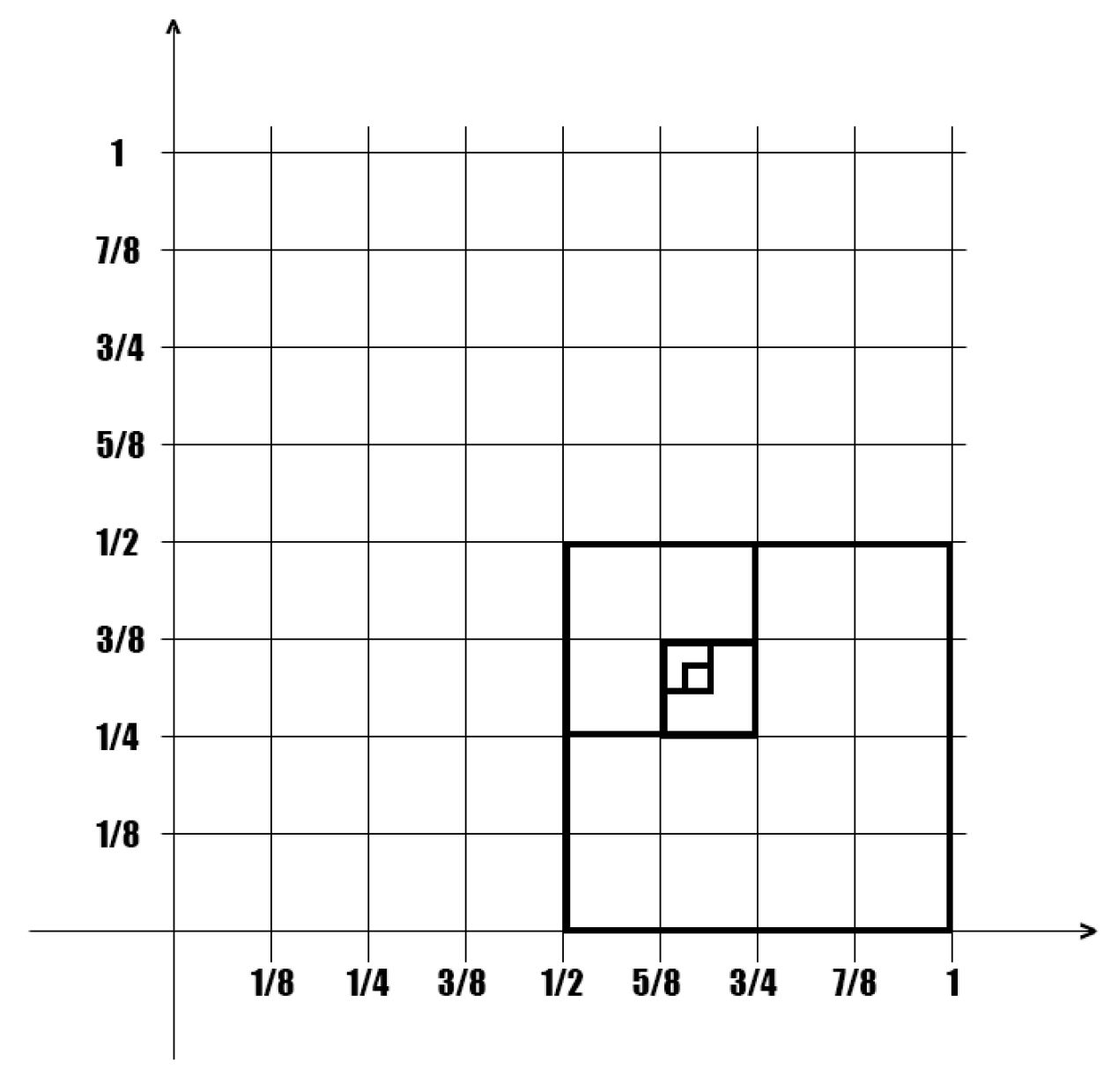
with $\alpha \ge 1$ and $0<\gamma \le 1$. We will also suppose that there are no columns with only zeros in any of the substitution matrices, which implies that there exists $ϵ>0$ such that $x_j>ϵ$. The parameters $\alpha$ and $\gamma$ will be chosen to satisfy certain conditions ahead. In order to define the random surface we take a partition of ${]0,1[}^2$ by a sequence of dyadic cells. A representation of a decreasing sequence of dyadic cells in ${]0,1[}^2$ is given in Figure 4.

In order to link the column random variables of the sequence ${\left(L_j\right)}_{j\ge 1}$ to the dyadic cells we consider for each decreasing sequence of dyadic cells such as:

$$C={\left(c(i_1,i_1{i}_2,i_1{i}_2{i}_3,\cdots ,i_1{i}_2{i}_3\cdots i_N)\right)}_{N\ge 1}$$

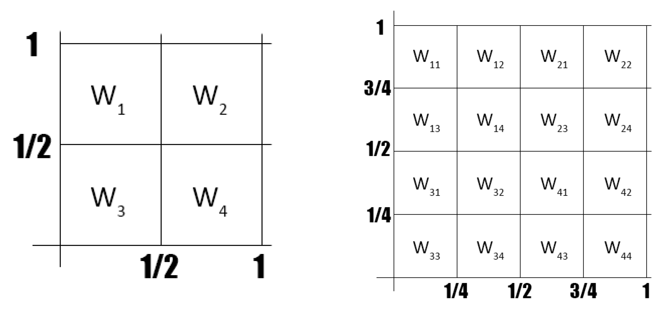
which is uniquely identified by the indexes identifying the decreasing sequence of dyadic cells $i_1$, $i_1{i}_2$, $i_1{i}_2{i}_3$, ⋯, $i_1{i}_2{i}_3\cdots i_N$, ⋯, $i_1,i_2,i_3,\cdots ,i_N,\cdots \in \{1,2,3,4\}$. We have the following algorithm to rename the column random variables of the sequence ${\left(L_j\right)}_{j\ge 1}\equiv {\left(L_j\left(\alpha \right)\right)}_{j\ge 1}$:

$$\begin{array}{cccc}{W}_1=L_1& W_2=L_2& W_3=L_3& W_4=L_4\\ W_{1,1}=L_5& W_{1,2}=L_6& W_{1,3}=L_7& W_{1,4}=L_8\\ W_{2,1}=L_9& W_{2,2}=L_{10}& W_{2,3}=L_{11}& W_{2,4}=L_{12}\\ W_{3,1}=L_{13}& W_{3,2}=L_{14}& W_{3,3}=L_{15}& W_{3,4}=L_{16}\\ W_{4,1}=L_{17}& W_{4,2}=L_{18}& W_{4,3}=L_{19}& W_{4,4}=L_{20}\cdots \end{array}$$

The linking algorithm of the column random variables to the dyadic cells of ${[0,1]}^2$ in its first step and second steps is as indicated in Figure 5.

We now detail the sequence of random variables that give the height of the random surface. For that purpose we define a sequence of random variables ${\left(M_N\right)}_{n\ge 1}$ uniquely associated with a decreasing sequence of dyadic cells in the following way:

$$M_N=M_N\left(c(i_1,i_1{i}_2,\cdots ,i_1{i}_2\cdots i_N)\right):=W_{i_1}·W_{i_1{i}_2}·W_{i_1{i}_2{i}_3}\cdots W_{i_1{i}_2{i}_3\cdots i_N}=\prod _{k=1}^N{W}_{i_1{i}_2{i}_3\cdots i_k},$$

(28)

observing that $M_N=M_N\left(c(i_1,i_1{i}_2,\cdots ,i_1{i}_2\cdots i_N)\right)$ with $c(i_1,i_1{i}_2,\cdots ,i_1{i}_2\cdots i_N)$ the finite sequence of dyadic cells that goes until the Nth step. We further observe that for every $(s,t)\in ]0,1[\times ]0,1[$ there exists an unique sequence $C(s,t)={\left(c(i_1,i_1{i}_2,\cdots ,i_1{i}_2\cdots i_N)\right)}_{N\ge 1}$ of decreasing dyadic cells such that:

$$\left\{(s,t)\right\}=\bigcap _{N\ge 1}c(i_1,i_1{i}_2,i_1{i}_2{i}_3,\cdots ,i_1{i}_2{i}_3\cdots i_N)$$

This decreasing sequence of dyadic cells of a given point allows, with an additional hypothesis, the definition of the random surface via the sequence ${\left(M_N\right)}_{N\ge 1}=(M_N{\left(C(s,t)\right)}_{N\ge 1}$.

Consider the left (negative) tail average for the distribution of $X_{i,j}^{m_{i,j}}$ given by:

$$a_{i,j}:=-{\int }_{-\infty }^{0}xd{F}_{X_{i,j}^{m_{i,j}}}\left(x\right).$$

We have the following result.

Theorem 7

(Existence of a nontrivial random field associated with a structured random matrix). Suppose that the following assumptions are verified:

(a) 

The left tail averages verify:

$$\sum _{i=1}^{\infty }\frac{a_{i,j}}{p^i}\le m<+\infty ,$$

for some constant m.

(b) 

The variances of the random variables $X_{i,j}^{m_{i,j}}$ verify $\mathbb{V}\left[X_{i,j}^{m_{i,j}}\right]=x_j^{2{\alpha }_0}·v_i$, for a certain ${\alpha }_0={\alpha }_0\left(m\right)$ to be determined later and with $v_i$ such that:

$$1<V:=\sum _{i=1}^{\infty }\frac{v_i}{p^{2i}}<+\infty .$$

Then, there is a combination of the parameters $\alpha ,\gamma$ such that, for each $(s,t)\in ]0,1[\times ]0,1[$ the sequence ${\left(M_N\right)}_{N\ge 1}=(M_N{\left(C(s,t)\right)}_{N\ge 1}$ is a supermartingale that converges almost surely to a random variable $X_{(s,t)}$ defining the random field ${\left(X_{(s,t)}\right)}_{(s,t)\in {]0,1[}^2}$, that is:

$$X_{(s,t)}:=\underset{N\to +\infty }{lim}{M}_N\left(c(i_1,i_1{i}_2,\cdots ,i_1{i}_2\cdots i_N)\right)a.s.,$$

(29)

and $\mathbb{E}\left[|X_{(s,t)}|\right]<+\infty$. Moreover, $\mathbb{V}\left[X_{(s,t)}\right]\ge 1$, that is, the random variable $X_{(s,t)}$ is not constant.

Proof. 

We first observe that since $x_j\ge ϵ$ we have:

$$\mathbb{E}\left[|L_j(\alpha ,\gamma )|\right]\le \frac{\gamma }{x_j^{\alpha }}\left(\sum _{i=1}^{+\infty }\frac{\mathbb{E}\left[|X_{i,j}^{m_{i,j}}|\right]}{p^i}\right)=\frac{\gamma }{x_j^{\alpha }}\left(\sum _{i=1}^{+\infty }\frac{m_{i,j}+a_{i,j}}{p^i}\right)\le \gamma \frac{1+m}{{ϵ}^{\alpha }}.$$

We now choose $\alpha ={\alpha }_0$ such that $(1+m)/{ϵ}^{\alpha }\le 1$. Due to the independence of the of the random variables $X_{i,j}^{m_{i,j}}$, we have that:

$$\mathbb{V}\left[L_j\right]=\frac{{\gamma }^2}{x_j^{2{\alpha }_0}}\sum _{i=1}^{+\infty }\frac{\mathbb{V}\left[X_{i,j}^{m_{i,j}}\right]}{p^{2i}}=\frac{{\gamma }^2}{x_j^{2{\alpha }_0}}\sum _{i=1}^{+\infty }\frac{x_j^{2{\alpha }_0}·v_i}{p^{2i}}={\gamma }^{2}V.$$

We now choose $\gamma ={\gamma }_0\le 1$ such that ${\gamma }_0^{2}V=1$. The random variables of the sequence ${(W_{i_1},W_{i_1{i}_2},W_{i_1{i}_2{i}_3},\cdots W_{i_1{i}_2{i}_3\cdots i_N})}_{N\ge 1}$ are, in fact, distinct random variables of the sequence ${\left(L_j({\alpha }_0,{\gamma }_0)\right)}_{j\ge 1}$ and so, are independent. It is well known that, since

$$0\le \mathbb{E}\left[L_j({\alpha }_0,{\gamma }_0)\right]=\left|\mathbb{E}\left[L_j({\alpha }_0,{\gamma }_0)\right]\right|\le \mathbb{E}\left[|L_j({\alpha }_0,{\gamma }_0)|\right]\le 1,$$

a sequence such as the one defined by Formula (28) is a supermartingale with respect to its natural filtration (see, for instance, ([58], p. 475)). Due to the independence we have that:

$$\begin{array}{cc}\hfill \mathbb{E}\left[|M_N|\right]& =\mathbb{E}\left[|W_{i_1}|\right]·\mathbb{E}\left[|W_{i_1{i}_2}|\right]·\mathbb{E}\left[|W_{i_1{i}_2{i}_3}|\right]\cdots \mathbb{E}\left[|W_{i_1{i}_2{i}_3\cdots i_N}|\right]\hfill \\ \hfill & =\prod _{k=1}^N\mathbb{E}\left[|W_{i_1{i}_2{i}_3\cdots i_k}|\right]\le 1,\hfill \end{array}$$

that is, ${sup}_{N\ge 1}\mathbb{E}\left[|M_N|\right]\le 1$, and so, due to a well known theorem of Doob (see, for instance, ([58], p. 508)) the first conclusion follows. Using the facts that $\mathbb{V}\left[L_j({\alpha }_0,{\gamma }_0)\right]=1$ and that the random variables $W_{i_1{i}_2{i}_3\cdots i_k}$ are distinct elements of the sequence ${\left(L_j({\alpha }_0,{\gamma }_0)\right)}_{j\ge 1}$, observing that for $k\ne l$ we have that,

$$\begin{array}{cc}\hfill \mathbb{V}\left[L_k·L_l\right]& =\mathbb{V}\left[L_k\right]·\mathbb{V}\left[L_l\right]+\mathbb{V}\left[L_k\right]·\mathbb{E}{\left[L_l\right]}^2\mathbb{V}\left[L_l\right]·\mathbb{E}{\left[L_k\right]}^2\hfill \\ \hfill & =1+\mathbb{E}{\left[L_l\right]}^2+\mathbb{E}{\left[L_k\right]}^2\ge 1,\hfill \end{array}$$

by induction, we now can state that:

$$\mathbb{V}\left[M_N\right]=\mathbb{V}\left[\prod _{k=1}^N{W}_{i_1{i}_2{i}_3\cdots i_k}\right]\ge 1,$$

and so the second conclusion also follows. □

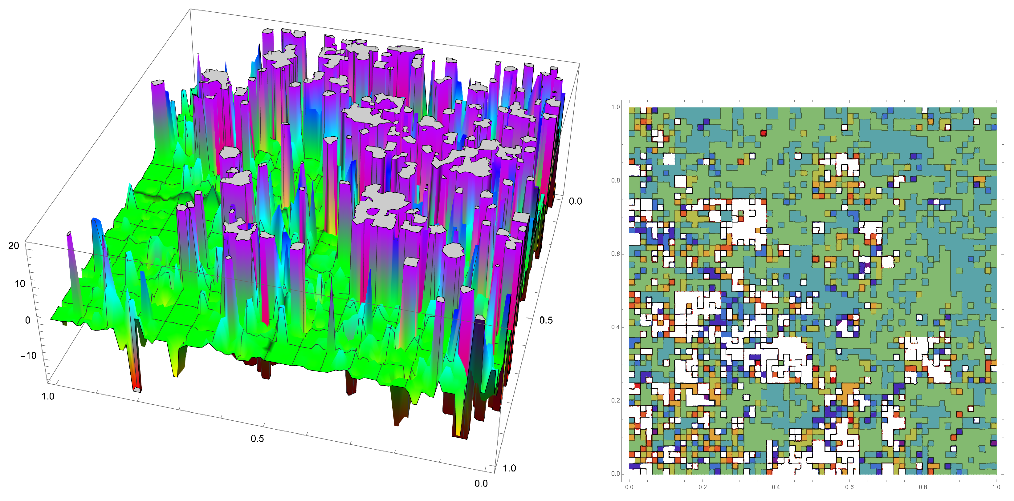
Let us give an idea of a random field built under the hypothesis of Theorem 7. In Figure 6, we present a low order approximation of the random surface associated with the example introduced by Formula (1) in Section 2.1. The skeleton for this approximation is the matrix $M_7$ a square matrix having around 43 million entries.

Remark 18

(On the covariance of the random field ${\left(X_{(s,t)}\right)}_{(s,t)\in {]0,1[}^2}$). Due to the general procedure considered in the construction of the random field it is possible to determine some interesting results on the covariance. In fact let, for two distinct points $(s,t),(s^{\prime },t^{\prime })\in {]0,1[}^2$, be the correspondent martingale sequences with elements $M_N\left(C(s,t)\right)$ and $M_{N+P}\left(C(s^{\prime },t^{\prime })\right)$ with $N,P\ge 1$. Let us suppose that the integer $0\le N_0<N$ is the largest integer such that the points $(s,t),(s^{\prime },t^{\prime })$ both belong to the same dyadic cell. It is then clear then that:

$$\begin{array}{cc}\hfill & Cov\left[M_N\left(C(s,t)\right),M_{N+P}\left(C(s^{\prime },t^{\prime })\right)\right]\hfill \\ \hfill & =\mathbb{E}\left[M_{N_0}{\left(C(s,t)\right)}^2\right]\mathbb{E}\left[\prod _{k=N_0+1}^N{W}_{i_1{i}_2{i}_3\cdots i_k}\left(C(s,t)\right)\right]\mathbb{E}\left[\prod _{k=N_0+1}^{N+P}{W}_{i_1{i}_2{i}_3\cdots i_k}\left(C(s^{\prime },t^{\prime })\right)\right]\hfill \\ \hfill & -\mathbb{E}\left[M_N\left(C(s,t)\right)\right]\mathbb{E}\left[M_{N+P}\left(C(s^{\prime },t^{\prime })\right)\right].\hfill \end{array}$$

If all the random variables of the sequence ${\left(L_j\right)}_{j\ge 1}$ have mean equal to 1 and then, forcefully, the absolute moment of second order is strictly larger than 1, for instance, equal to 2, then, again by Lebesgue convergence theorem we have that:

$$Cov\left[X_{(s,t)},X_{(s^{\prime },t^{\prime })}\right]=2^{N_0}-1,$$

where, as already said, $N_0\ge 0$ is the largest integer such that the points $(s,t),(s^{\prime },t^{\prime })$ both belong to the same dyadic cell. If the points do not belong to any common dyadic cell (see Figure 5), that is if $N_0=0$, the covariance is null. The closer the points are, the larger the integer $N_0$ is, and so, the larger the covariance.

5. Conclusions and Future Work

In this work, we introduced structured random matrices having a skeleton built from the a matrix substitution process with entries in a finite field. We showed that the iterated application of a particular kind of matrix substitution generates a sequence of matrices that admit a periodic point—that may be a fixed point—or a fixed point for the sequence of matrix principal parts of a given order. The random matrices, with independent entries, having as skeletons matrices derived from this matrix substitution process have remarkable properties whenever the random variables satisfy some uniform properties. It is showed, under adequate hypothesis, that:

• The existence of a particular type of structure of matrix substitution type is identifiable by simple statistical procedures;
• The convergence in law of a sequence of random matrices having as skeletons a sequence of matrices with entries in a finite field that, of matrix substitution type, converges to a fixed point;
• There is a generic result on the spectral analysis for the random matrices derived from a matrix substitution procedure;
• There is a canonical manner to associate a nontrivial random field with interesting properties to a random matrix having as a skeleton a matrix with entries in a finite field of matrix substitution type.

A more detailed analysis of the spectral properties of the random matrices here introduced is, for us, open to future work. Furthermore, matrices with a high percentage of zeros can be generated by considering special global matrix substitutions maps; the detailed properties of these matrices will be object of future work. Finally, a reciprocal problem to the one considered in this work is to determine if a large matrix is a fixed point of some global matrix substitution map. A reasonable conjecture is that for every large matrix there exists a global matrix substitution map admitting a fixed point that is close, in some sense, to the given matrix.

References

1. Liu, S.; McGree, J.; Ge, Z.; Xie, Y. Computational and Statistical Methods for Analysing Big Data with Applications; Elsevier: Amsterdam, The Netherlands; Academic Press: Cambridge, MA, USA, 2016; pp. 11 + 194. [Google Scholar]
2. Pytheas Fogg, N.; Berthé, V.; Ferenczi, S.; Mauduit, C.; Siegel, A. (Eds.) Substitutions in Dynamics, Arithmetics and Combinatorics; Springer: Berlin/Heidelberg, Germany, 2002; Volume 1794, pp. 15 + 402. [Google Scholar] [CrossRef]
3. Queffélec, M. Substitution Dynamical Systems. Spectral Analysis, 2nd ed.; Springer: Dordrecht, The Netherlands, 2010; Volume 1294, pp. 15 + 351. [Google Scholar] [CrossRef]
4. von Haeseler, F. Automatic Sequences; Walter de Gruyter: Berlin/Heidelberg, Germany, 2003; pp. 6 + 191. [Google Scholar]
5. Allouche, J.P.; Shallit, J. Automatic Sequences; Theory, Applications, Generalizations; Cambridge University Press: Cambridge, UK, 2003; pp. 16 + 571. [Google Scholar] [CrossRef]
6. Frank, N.P. Multidimensional constant-length substitution sequences. Topol. Its Appl. 2005, 152, 44–69. [Google Scholar] [CrossRef]
7. Bartlett, A. Spectral theory of Zd substitutions. Ergod. Theory Dyn. Syst. 2018, 38, 1289–1341. [Google Scholar] [CrossRef]
8. Jolivet, T.; Kari, J. Consistency of multidimensional combinatorial substitutions. Theor. Comput. Sci. 2012, 454, 178–188. [Google Scholar] [CrossRef]
9. Fogg, N.P.; Berthé, V.; Ferenczi, S.; Mauduit, C.; Siegel, A. (Eds.) Polynomial dynamical systems associated with substitutions. In Substitutions in Dynamics, Arithmetics and Combinatorics; Springer: Berlin/Heidelberg, Germany, 2002; pp. 321–342. [Google Scholar]
10. Ginibre, J. Statistical ensembles of complex, quaternion, and real matrices. J. Math. Phys. 1965, 6, 440–449. [Google Scholar] [CrossRef]
11. Girko, V. Theory of Random Determinants; Translated from the Russian; Kluwer Academic Publishers: Dordrecht, The Netherlands, 1988; pp. 25 + 677. [Google Scholar]
12. Girko, V. Statistical Analysis of Observations of Increasing Dimension; Translated from the Russian; Kluwer Academic Publishers: Dordrecht, The Netherlands, 1995; pp. 21 + 286. [Google Scholar]
13. Bai, Z.D. Methodologies in Spectral Analysis of Large Dimensional Random Matrices, a review. Stat. Sin. 1999, 9, 611–662. [Google Scholar]
14. Götze, F.; Tikhomirov, A. The circular law for random matrices. Ann. Probab. 2010, 38, 1444–1491. [Google Scholar] [CrossRef]
15. Alexeev, N.; Götze, F.; Tikhomirov, A. Asymptotic distribution of singular values of powers of random matrices. Lith. Math. J. 2010, 50, 121–132. [Google Scholar] [CrossRef]
16. Götze, F.; Naumov, A.; Tikhomirov, A. Distribution of linear statistics of singular values of the product of random matrices. Bernoulli 2017, 23, 3067–3113. [Google Scholar] [CrossRef]
17. Götze, F.; Naumov, A.; Tikhomirov, A.; Timushev, D. On the local semicircular law for Wigner ensembles. Bernoulli 2018, 24, 2358–2400. [Google Scholar] [CrossRef]
18. Götze, F.; Tikhomirov, A. Rate of convergence in probability to the Marchenko-Pastur law. Bernoulli 2004, 10, 503–548. [Google Scholar] [CrossRef]
19. Mehta, M.L. Random Matrices, 3rd ed.; Pure and Applied Mathematics (Amsterdam); Elsevier: Amsterdam, The Netherlands; Academic Press: Cambridge, MA, USA, 2004; Volume 142, pp. 18 + 688. [Google Scholar]
20. Anderson, G.W.; Guionnet, A.; Zeitouni, O. An Introduction to Random Matrices; Cambridge Studies in Advanced Mathematics; Cambridge University Press: Cambridge, UK, 2010; Volume 118, pp. 14 + 492. [Google Scholar]
21. Guionnet, A. Grandes matrices aléatoires et théorèmes d’universalité (d’après Erdos, Schlein, Tao, Vu et Yau). Astérisque 2011, 1, 203–237. [Google Scholar]
22. Tao, T. Topics in Random Matrix Theory; Graduate Studies in Mathematics; American Mathematical Society: Providence, RI, USA, 2012; Volume 132, pp. 10 + 282. [Google Scholar] [CrossRef]
23. Vu, V.H. (Ed.) Modern aspects of random matrix theory. In Proceedings of the Symposia in Applied Mathematics, San Diego, CA, USA, 6–7 January 2013; Papers from the AMS Short Course on Random Matrices. American Mathematical Society: Providence, RI, USA, 2014; Volume 72, pp. 8 + 174. [Google Scholar] [CrossRef]
24. Akemann, G.; Baik, J.; Di Francesco, P. (Eds.) The Oxford Handbook of Random Matrix Theory; Paperback edition of the 2011 original [MR2920518]; Oxford University Press: Oxford, UK, 2015; pp. 31 + 919. [Google Scholar]
25. Erdos, L.; Yau, H.T. A Dynamical Approach to Random Matrix Theory; Courant Lecture Notes in, Mathematics; Courant Institute of Mathematical Sciences: New York, NY, USA; American Mathematical Society: Providence, RI, USA, 2017; Volume 28, pp. 9 + 226. [Google Scholar]
26. Banerjee, D.; Bose, A. Patterned sparse random matrices: A moment approach. Random Matrices Theory Appl. 2017, 6, 1750011. [Google Scholar] [CrossRef]
27. Bose, A. Patterned Random Matrices; CRC Press: Boca Raton, FL, USA, 2018; pp. 21 + 267. [Google Scholar] [CrossRef]
28. Livshyts, G.V.; Tikhomirov, K.; Vershynin, R. The smallest singular value of inhomogeneous square random matrices. Ann. Probab. 2021, 49, 1286–1309. [Google Scholar] [CrossRef]
29. Jain, V.; Silwal, S. A note on the universality of ESDs of inhomogeneous random matrices. ALEA Lat. Am. J. Probab. Math. Stat. 2021, 18, 1047–1059. [Google Scholar] [CrossRef]
30. Tikhomirov, A.N. On the Wigner law for generalizided random graphs. Sib. Adv. Math. 2021, 31, 301–308. [Google Scholar] [CrossRef]
31. Liu, Y.; Chen, A.; Lin, F. Threshold function of ray nonsingularity for uniformly random ray pattern matrices. Linear Multilinear Algebra 2022, 70, 5708–5715. [Google Scholar] [CrossRef]
32. Ali, M.S.; Srivastava, S.C.L. Patterned random matrices: Deviations from universality. J. Phys. A 2022, 55, 495201. [Google Scholar] [CrossRef]
33. Bernkopf, M. A history of infinite matrices. A study of denumerably infinite linear systems as the first step in the history of operators defined on function spaces. Arch. History Exact Sci. 1968, 4, 308–358. [Google Scholar] [CrossRef]
34. Shivakumar, P.N.; Sivakumar, K.C. A review of infinite matrices and their applications. Linear Algebra Appl. 2009, 430, 976–998. [Google Scholar] [CrossRef]
35. Williams, J.J.; Ye, Q. Infinite matrices bounded on weighted 1 spaces. Linear Algebra Appl. 2013, 438, 4689–4700. [Google Scholar] [CrossRef]
36. Lindner, M. Infinite Matrices and Their Finite Sections; Frontiers in Mathematics; An introduction to the limit operator method; Birkhäuser Verlag: Basel, Switzerland, 2006; pp. 15 + 191. [Google Scholar]
37. Warusfel, A. Structures Algébriques Finies. Groupes, Anneaux, Corps; Collection Hachette Université, Librairie Hachette: Paris, France, 1971; p. 271. [Google Scholar]
38. Koan, V.K. Distributions, Analyse de Fourier, Opérateurs aux Dérivées Partielles; Number tome 1 in Cours et exercices résolus maîtrise de mathématiques: Certficat C2; Vuibert: Paris, France, 1972. [Google Scholar]
39. Schaefer, H.H. Topological Vector Spaces; Springer: New York, NY, USA, 1971; Volume 3. [Google Scholar]
40. Köthe, G. Topological Vector Spaces. I; Die Grundlehren der mathematischen Wissenschaften in Einzeldarstellungen. 159; Garling, D.J.H., Translator; Springer: Berlin/Heidelberg, Germany; New York, NY, USA, 1969; pp. 15, 456. [Google Scholar]
41. Skorohod, A.V. Random Linear Operators; Mathematics and its Applications (Soviet Series); Translated from the Russian; D. Reidel Publishing Co.: Dordrecht, The Netherlands, 1984; pp. 16 + 199. [Google Scholar] [CrossRef]
42. Guo, T.X. Extension theorems of continuous random linear operators on random domains. J. Math. Anal. Appl. 1995, 193, 15–27. [Google Scholar] [CrossRef]
43. Thang, D.H.; Thinh, N. Generalized random linear operators on a Hilbert space. Stochastics 2013, 85, 1040–1059. [Google Scholar] [CrossRef]
44. Quy, T.X.; Thang, D.H.; Thinh, N. Abstract random linear operators on probabilistic unitary spaces. J. Korean Math. Soc. 2016, 53, 347–362. [Google Scholar] [CrossRef]
45. Chiu, S.N.; Liu, K.I. Generalized Cramér-von Mises goodness-of-fit tests for multivariate distributions. Comput. Stat. Data Anal. 2009, 53, 3817–3834. [Google Scholar] [CrossRef]
46. Thas, O. Comparing Distributions; Springer: New York, NY, USA, 2010; pp. 18 + 353. [Google Scholar]
47. McAssey, M.P. An empirical goodness-of-fit test for multivariate distributions. J. Appl. Stat. 2013, 40, 1120–1131. [Google Scholar] [CrossRef]
48. Fan, Y. Goodness-of-Fit Tests for a Multivariate Distribution by the Empirical Characteristic Function. J. Multivar. Anal. 1997, 62, 36–63. [Google Scholar] [CrossRef]
49. Shiryaev, A.N. Probability. 1, 3rd ed.; Boas, R.P., Chibisov, D.M., Eds.; Graduate Texts in Mathematics; Translated from the fourth (2007) Russian; Springer: New York, NY, USA, 2016; Volume 95, pp. 17 + 486. [Google Scholar]
50. Kallenberg, O. Foundations of Modern Probability; Probability Theory and Stochastic Modelling; Third edition [of 1464694]; Springer: Cham, Switzerland, 2021; Volume 99, pp. 12 + 946. [Google Scholar] [CrossRef]
51. Gel’fand, I.M.; Vilenkin, N.Y. Generalized Functions. Vol. 4: Applications of Harmonic Analysis; Translated by Amiel Feinstein; Academic Press: New York, NY, USA; London, UK, 1964; pp. 14 + 384. [Google Scholar]
52. Gohberg, I.; Goldberg, S. Basic Operator Theory; Birkhäuser: Boston, MA, USA, 1980; pp. 13 + 285. [Google Scholar]
53. Billingsley, P. Probability and Measure, 3rd ed.; Wiley Series in Probability and Mathematical Statistics; A Wiley-Interscience Publication; John Wiley & Sons, Inc.: New York, NY, USA, 1995; pp. 14 + 593. [Google Scholar]
54. Kahane, J.P.; Peyrière, J. Sur certaines martingales de Benoit Mandelbrot. Adv. Math. 1976, 22, 131–145. [Google Scholar] [CrossRef]
55. Lévy, P. Esquisse d’une théorie de la multiplication des variables aléatoires. Ann. Sci. École Norm. Sup. 1959, 76, 59–82. [Google Scholar] [CrossRef]
56. Zolotarev, V.M. General theory of the multiplication of random variables. Dokl. Akad. Nauk SSSR 1962, 142, 788–791. [Google Scholar]
57. Simonelli, I. Convergence and symmetry of infinite products of independent random variables. Statist. Probab. Lett. 2001, 55, 45–52, Erratum in Statist. Probab. Lett. 2003, 62, 323. [Google Scholar] [CrossRef]
58. Shiryaev, A.N. Probability, 2nd ed.; Graduate Texts in Mathematics; Translated from the first (1980) Russian edition by R. P. Boas; Springer: New York, NY, USA, 1996; Volume 95, pp. 16 + 623. [Google Scholar] [CrossRef]
Figure 1. Histogram of absolute values of the eigenvalues of the structured matrices R 7 and M 7 .
Mathematics 11 02505 g001
Figure 2. Dispersion or real and imaginary parts of eigenvalues of R 7 and M 7 .
Mathematics 11 02505 g002
Figure 3. Eigenvalues distribution in C of a sample of 40 matrices with affine substitution induced structure and increasing variance.
Mathematics 11 02505 g003
Figure 4. A decreasing sequence of dyadic cells.
Mathematics 11 02505 g004
Figure 5. The placement of the first four random variables: first step (left); The placement of the next 16 random variables: second step (right).
Mathematics 11 02505 g005
Figure 6. An approximation of low order of the random surface, built upon the skeleton M 7 : surface plot (left); Contour plot: (right).
Mathematics 11 02505 g006
Disclaimer/Publisher’s Note: The statements, opinions and data contained in all publications are solely those of the individual author(s) and contributor(s) and not of MDPI and/or the editor(s). MDPI and/or the editor(s) disclaim responsibility for any injury to people or property resulting from any ideas, methods, instructions or products referred to in the content.