Development of CAVLAB—A Control-Oriented MATLAB Based Simulator for an Underground Coal Gasification Process

Abstract

The Cavity Simulation Model (CAVSIM) is a 3D, parameterisable simulator of the Underground Coal Gasification Process (UCG) that serves as a benchmark for UCG prediction. Despite yielding accurate outputs, CAVSIM has some limitations, which chiefly include inadequate graphical capabilities to visualise cavity geometry and gas production, time-ineffectiveness in terms of parametrisation, i.e., it involves editing, compiling multiple files and checking for errors, and lack of tools to synthesise a controller. Therefore, to compensate for these shortcomings, the services of third-party software, such as MATLAB, must be procured. CAVSIM was integrated with MATLAB to utilise its functionalities and toolboxes such as System Identification, Neural Network, and Optimization Toolbox etc. The integration was accomplished by designing C-mex files, and furthermore, the simulation results in both environments exhibit the same behaviour, demonstrating successful integration. Consequently, CAVSIM has also acquired a controllable structure, wherein parametrisation is now a single-click process; this is demonstrated by a case study outlining the implementation of Model Predictive Control (MPC) on a UCG plant. Moreover, the performance metrics, i.e., Mean Average Error (MAE) and Root Mean Square Error (RMSE) of 0.13, 0.23 for syngas heating value, and 0.012, 0.02 for flowrate quantitatively establishes the efficacy of CAVLAB in designing MPC for the UCG system. The novelty of this work lies in making the software package open-source with the aim of streamlining the research of multiple aspects of the UCG process.

1. Introduction

The Underground Coal Gasification (UCG) process is an in-situ procedure wherein the coal reserves that are buried deep inside the earth’s layers are accessed through specially drilled wells, cf. Figure 1. Furthermore, the 600 billion tonnes of underground coal reserves (most of which are un-minable) make it an appealing alternative energy source in a world that is rapidly depleting its natural resources and becoming increasingly conscious of its climate [1]. However, hurdles such as geo-physical, environmental, and controller design have impeded the UCG process from making significant contributions to the energy sector [2]. This work, thereby, aims to address a specific theoretical design constraint that is primarily related to UCG modelling, simulation and control.

1.1. Motivation

Mathematical modelling has a pivotal role in modern science and technology. A well-developed model can not only predict the system’s behaviour but also help control its output. Similarly, there has been a shift in the burden of calculation from the user’s end to the computer’s due to a boom in the emergence of computational software, such as ANSYS, COMSOL, and ANYLOGIC, to name a few. These software tools enable the user to simulate complex systems and scenarios with high accuracy and efficiency [3]. They also reduce the cost and time required for physical experiments and testing. Moreover, they allow the user to explore various parameters and optimize the system’s performance [4,5]. However, most of them are tailored to address the specific streams of science and technology, and there is no under-one-roof software to cater to all the needs of any design project. In this regard, the gap created by the lack of interaction between software has to be bridged by developing some sort of interface. In some instances, developers of high-end commercial software have provided a built-in interface or plugins to integrate two software, e.g., SOLIDWORKS-Simscape Multibody, ANSYS-MATLAB, and MSC Adams-MATLAB, the application of which is illustrated by [6]; however, at other instances, such functionalities are not natively available. In this work, we are going to introduce Cavity Laboratory (CAVLAB), which was engendered by integrating Cavity Simulation (CAVSIM) with MATLAB. CAVSIM is a 3D, parameterisable, multiphysics simulator of the Underground Coal Gasification (UCG) process that emulates and predicts the UCG plant’s outputs, such as syngas’s heating value and flowrate, and cavity growth with high accuracy [7]. It performs the UCG simulation by solving a set of partial differential equations that represent the changes in mass, momentum, and energy in the coal and the cavity. It also considers the different chemical reactions that take place during UCG, such as the decomposition, conversion,n and burning of coal. CAVSIM uses a numerical method with a finite difference approach and an implicit scheme to find the solutions to the equations. It also uses a technique that moves the boundary to follow the cavity expansion and adjusts the grid accordingly. However, despite yielding accurate results, as substantiated in our previous works [8,9], CAVSIM has certain shortcomings from the end-user’s perspective. Figure 1 holistically illustrates the simulation of the UCG process along with the shortcomings in CAVSIM. Moreover, an illustrative example, in the next paragraph outlining the CAVSIM’s workings and functionalities, is presented to fully comprehend the difficulties that a researcher may face when operating the simulator. Therefore, to streamline the process of simulating, system identification, and controller design for a UCG process using CAVSIM, it is imperative that it be integrated with third-party software.

Consider an open-loop UCG process that is described and simulated by CAVSIM as illustrated in part (a) of Figure 2. A control engineer might be interested in the following aspects: analysing the behaviour of the UCG process for various operating conditions, visually perceiving the system’s output at some specific design conditions, and designing a controller based on the system’s dynamics. The logical flow of the deployment of these steps in CAVSIM constitutes the following, as illustrated in part (b) of Figure 2: parametrisation and input signal design; simulation and data-logging for visualising the results; and designing and introducing controller in the simulation loop; wherein parametrisation means defining the UCG’s reactor properties, such as the coalbed’s chemical composition and its depth from the ground, etc., and the rest of the terms are self-explanatory. For this particular problem, all these steps take place in sequential order. However, due to notable limitations of the simulator and FORTRAN language, the deployment of these steps leads to severe difficulties. The reasons behind these limitations and the proposed solution are described as follows.

Firstly, to implement different design scenarios, as alluded to in the previous paragraph, a customised programming language or toolboxes are required, which are absent in CAVSIM. Although some design aspects, such as synthesising a classical controller, are possible, their implementation requires learning and gaining experience in FORTRAN, which is time-consuming and non-trivial considering the scant advantages it can yield, as demonstrated in our earlier works [10,11]. Thus, it is not well suited and equipped to tackle different design scenarios. Consequently, to add flexibility in UCG’s simulation pipeline and expand the scope of its research, it is recommended to integrate CAVSIM with third-party software, like MATLAB (the advantages of running CAVSIM in MATLAB are illustrated in Figure 1), whose functionalists can outright be utilised by invoking its toolboxes such as Neural Networks, Model Predictive Control (MPC) etc. [12,13].

1.2. Literature Review

Based on the theme of the current work, we have divided our literature overview into two themes: mathematical models available for UCG systems and a systematic review of works where integration between two software systems has been performed, the schemes used to perform integration, and the scope and limitations of the resulting integration.

The UCG process combines different physical domains, such as chemical kinetics, computational fluid dynamics, stress analysis, and thermodynamics. Therefore models derived are constrained by scope, assumptions, predictive capabilities, and physics; whilst simplifications include dimension and time response, heat transfer and fluid dynamics couplings, and predictive range, such as cavity evolution and environmental interaction. Based on these criteria, the UCG models can be categorized into the following groups: packed bed models [14,15,16,17], channel models [18,19,20], coal block models [21,22,23], resource recovery models [24,25], and CFD [26].

Packed bed, channel, and coal block models are suitable for lab experiments but lack the ability to simulate cavity shapes due to the absence of a thermo-mechanical failure module. Using numerical methods and data structures, computational fluid dynamics (CFD) is a branch of fluid mechanics that investigates and solves problems involving fluid flows. CFD can reveal the underlying transport phenomena in chemical and biochemical processes, such as heat, momentum, or mass transfer [27]. CFD can also assist in the design of various reactor types by providing insights on, for example, stirrer geometry or baffle shape, heat exchange area, or the required power input [28]. CFD models offer more realism and comprehensiveness, incorporating three-dimensional flow, heat/mass transfer, reactions, and cavity expansion in UCG. However, CFD models are complex and computationally intensive. CAVSIM, a resource recovery model, has advantages, such as modelling vertical and horizontal cavity expansion and accommodating various stratigraphy, coal properties, and overburden characteristics. Moreover, it has been validated through lab and field UCG experiments. Consequently, CAVSIM is a reliable and adaptable model for UCG simulation that must be integrated with MATLAB to lend it a controllable structure and access to toolboxes.

From this point onward, we are going to divert to the other theme of this work: integration between two software. Mahseredjian et al. [29] developed a programmed link between MATLAB and Electromagnetic Transient Program (EMTP) to utilise the former’s built-in functionalities. By using the MATLAB provided C and FORTRAN subroutines that externally allow access to its computational engine, MATLAB built-in functions were accessed. To start and stop MATLAB as an engine, an ‘engine control’ call was used. Despite the apparent advantage of versatility in types of data that can be exchanged, this method, however, has two obvious disadvantages: to gain access to discrete MATLAB functions, a separate user-defined m-file has to be written. There exists at least a unit-time delay whilst the data exchange takes place. Ahsan and Saramaki [30] implemented a Parks–McClellan (PM) algorithm, which is used to design a Finite-Impulse Response (FIR) filter. The original algorithm was written in FORTRAN, and the authors translated a part of it—Remez Multiple Exchange (RME)—into MATLAB’s code. Due to their faster operation speeds, vectors and matrices were used in the translated code, which displayed reduced execution time and reduced complexity than its FORTRAN counterpart. Bagal et al. [31] implemented a real-time control process by establishing an interface between MATLAB and SCADA. To achieve to and fro data transfer, KEPServerEX was used, which works as an Open Platform Communications Data Access (OPCDA) server working on a server-client architecture. The control problem was solved by first creating a Programmable Logic Controller (PLC) application. Second, programs in SCADA were integrated with processes via the OPC server. Finally, MATLAB/SIMULINK models were created to access and process data in run time. The test prototype was realised in hardware, and the results showed reliable data transfer among these packages: MATLAB, PLC, and SCADA. The obvious caveat to this and similar integration carried out by Ivan et al. [32] is the availability of a third-party connectivity platform, i.e., KEPServerEX, that can incur additional costs. Sokos et al. [33] developed a Graphical User Interface (GUI) in MATLAB for the ISOLA software package. The latter is the package developed for the inversion of local/regional seismograms of single and multi-point models by modelling an extended seismic source either as a point source or a collection of point sources. The package’s main computational routine is written in FORTRAN; however, to draw on the data-handling, graphics routine, and user-friendly capabilities of MATLAB, the authors incorporated the ISOLA package into MATLAB by developing a GUI. Moreover, they also demonstrated the package’s flexibility and adaptability in the integrated environment. Andersson et al. [34] have outlined the motivation, methodology, and working of Assimulo, which is a simulation framework for solving ODEs. At its core, Assimulo is the Python package, which is the amalgamation of various numerical solvers that solve the dynamical systems described by ODEs, DAEs, etc. To integrate solvers written in other programming languages with it, additional tools were used; for instance, for solvers written in C and FORTRAN, Cython, and F2PY that automatically invoke external codes into Python were used, respectively. Lee et al. [35] carried out the process of converting MT2DInv Magnetotelluric (MT) data into two dimensions using MT2DInvMatlab, an open-source MATLAB software suite. The package was created using a combination of MATLAB and FORTRAN. The main inversion takes place under MATLAB’s computation environment to visualise the inversion process, whereas some routines are written in FORTRAN to accelerate the computation process and re-use the pre-written FORTRAN legacy codes. Taking advantage of the mixed language environment afforded by MATLAB, they provided the FORTRAN code to generate MEX functions, providing an interface to integrate MATLAB with FORTRAN. Quaglia et al. [36] addressed the issue of the destabilisation of real-time systems that are interlinked with each other via packet networks. Such systems mostly destabilise due to packet losses and communication delays. To that end, they proposed a co-simulation framework comprising SystemC and MATLAB, wherein the former was used in protocol design and network simulation and later in controller synthesis. To build a channel between the two software, they used Kernel-based communication at SystemC’s end and wrapper function at MATLAB’s. Moreover, they demonstrated the efficacy of this framework by illustrating a case study of bilateral communication between the master device and a remotely operated slave robot. Hatledal et al. [37] developed a co-simulation platform called Vico that is based on the Entity-Component-System (ECS) architecture. Vico allows users to simulate and analyse complex systems by combining multiple simulation models and tools. The authors used the ECS architecture to represent the components and relationships within a system, which makes it easy to modify and extend the simulation. Vico also provides a GUI for building and running simulations, as well as a Python API for more advanced users. The authors conducted several case studies to demonstrate the capabilities and efficiency of Vico for co-simulating complex systems. In order to incorporate decision-making capability into the existing discrete-event simulators such as SIMIO, Dehghanimohammadabadi et al. [38] proposed integrating it with MATLAB. The intent was to deploy SIMIO as the simulation platform and MATLAB as the computational. To integrate, the API feature of SIMIO was used, wherein at each time instance, the simulation would pause, and MATLAB is invoked to leverage its toolboxes. In [39], authors aimed to assist researchers interested in simulating iron losses in electrical machines using COMSOL-Multiphysics and MATLAB. Their study demonstrated the feasibility of this approach by deriving model parameters from empirical data and applying them to COMSOL-Multiphysics and MATLAB through the use of MATLAB script code. Furthermore, they applied the method to various electric machine geometries and compared the results. However, it should be noted that this integration may lack scalability and is only an ad hoc solution for these specific problems and geometries.

The abovementioned literature review lays the motivational groundwork and sets the direction for building an interface between two programs, especially in situations where one of the programs’ routines is written in FORTRAN. The methodology, as construed from the literature review in its broad sense, boils down to three distinct ways: calling FORTRAN code from MATLAB, calling MATLAB from FORTRAN, and translating FORTRAN code into MATLAB m-file. Converting the FORTRAN code into MATLAB’s code is infeasible, particularly when the program spans thousands of lines of code. Moreover, this also requires an in-depth understanding of the data handling capabilities of both programming environments for a one-to-one mapping of the codes. Although there are open-source packages [40] that can perform the conversions, they have certain limitations in terms of dealing with complex read-and-write statements, derived-type variables, and equivalence statements and are not suitable for handling large codes. Regarding invoking MATLAB from FORTRAN, MATLAB Engine also enables programs in C, C++, or FORTRAN to interact with a separate MATLAB process through ActiveX on Windows. MATLAB Engine applications are independent programs that allow users to access MATLAB from their own FORTRAN programs, allowing them to use MATLAB as a computation engine. Since this method requires two processes running on a single machine, data transfer and computation become stagnant unless the user is working on a network and deploying other machines for computation.

Ultimately, calling FORTRAN from MATLAB requires creating MEX files. Compared to other methods, this is a fast mechanism as MATLAB treats the FORTRAN program as its m-file and does not rely on other processes. Moreover, unlike the Engine calling routine, this allows access to all MATLAB’s toolboxes. Though this path necessitates using third-party software, namely a FORTRAN compiler, the end-user product does not rely on any external software except MATLAB. Therefore, keeping in mind the ease of implementation and the subsequent use, we opted to perform the integration by this procedure.

1.3. Major Contributions and Overview

All in all, the major contributions of this work are enumerated as follows:

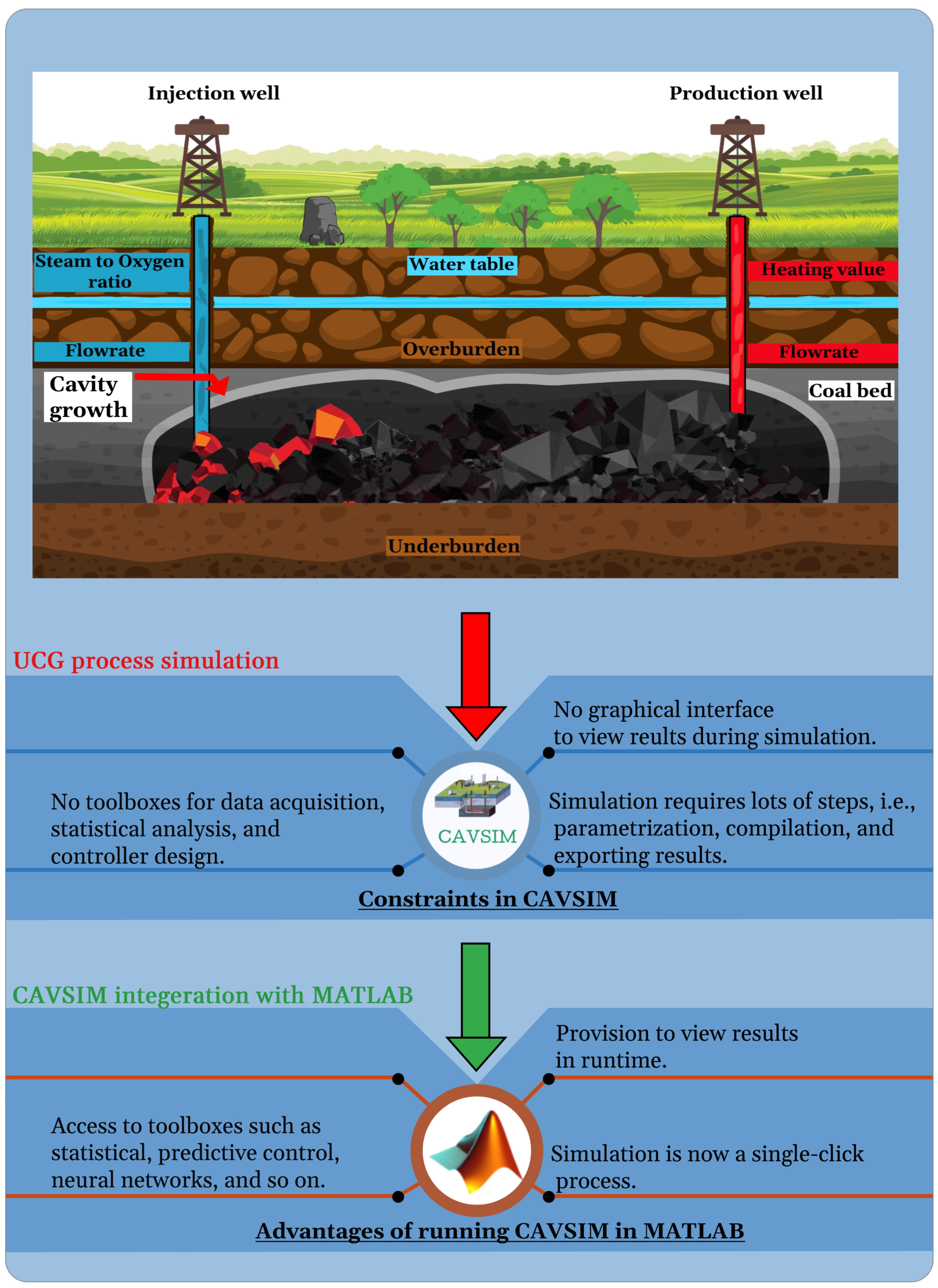
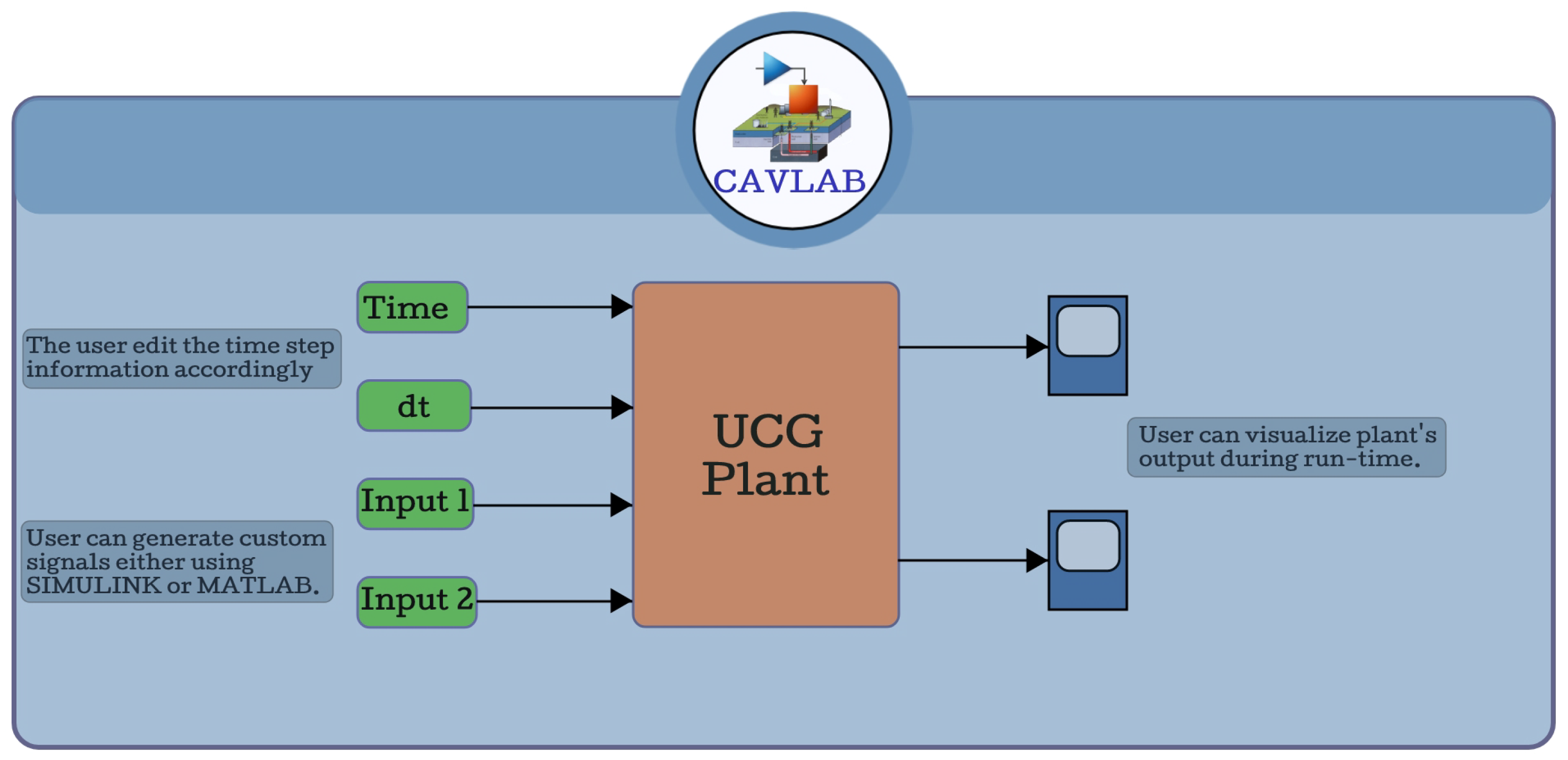
• The step-by-step development of CAVLAB—an augmented computational framework with a controllable structure for CAVSIM by integrating it with MATLAB. Beyond that, the additional structures appended to CAVSIM by virtue of integration constitute the following: ease of design and transmission of input signals; adjusting the plant’s parameters to simulate different variants of coal reactor is now just a one-click process; and provision to visualise the input and output data as the simulation is running.
• A case study of MPC design for UCG plant, demonstrating the ease of implementation and investigation of a UCG control design problem due to integration.
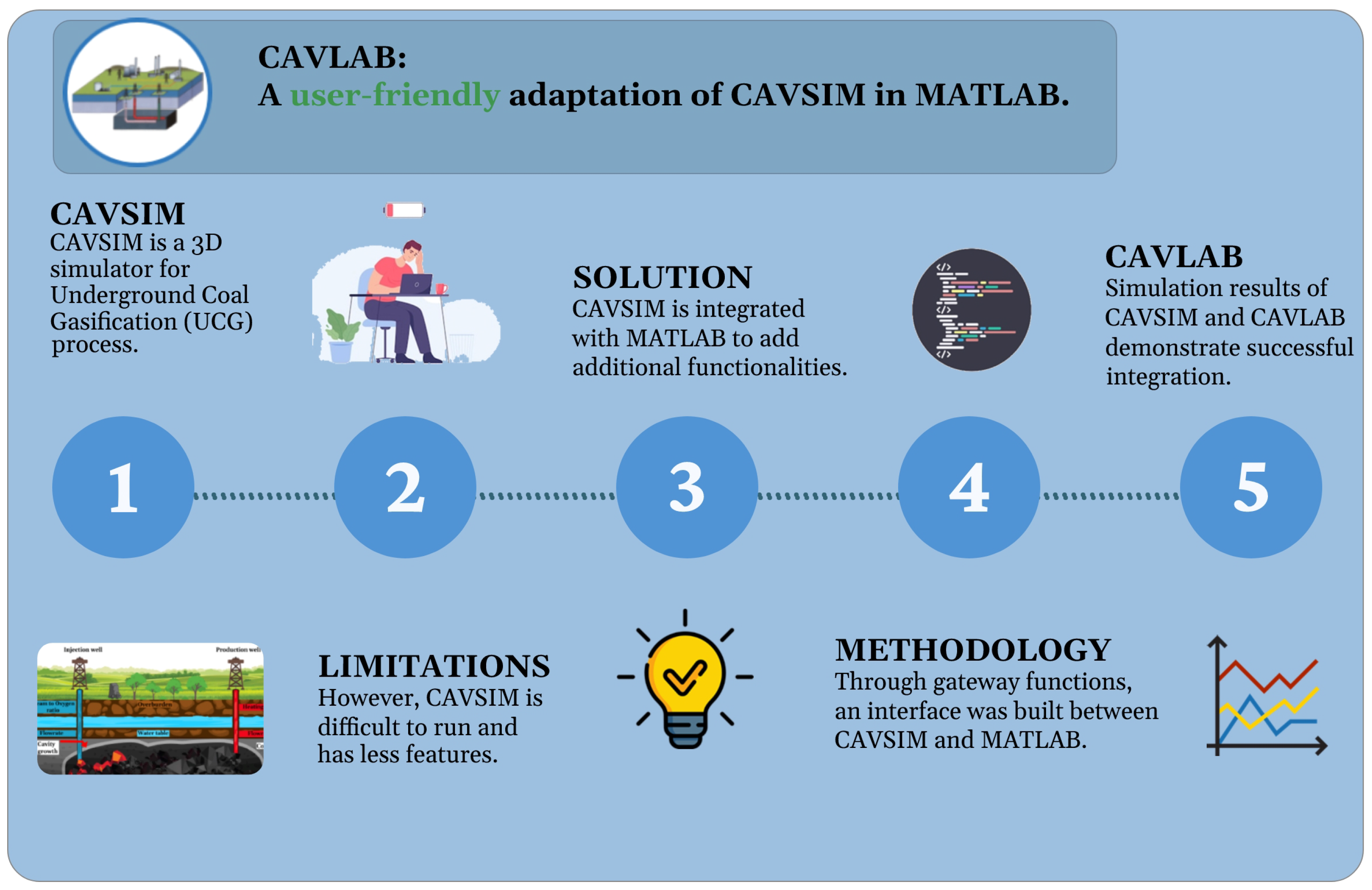
• CAVLAB has also been made available online, and to the best of our knowledge, this is the only software package that provides the capabilities of simulation, system identification, and optimal control of the UCG process.

To sum up, the objectives of the current work are as follows: CAVSIM is a UCG process that has limitations from the user’s perspective. It does not offer many features or options for modelling and simulation of underground coal gasification. To overcome this, CAVSIM was integrated with MATLAB, a powerful software for numerical computing and data analysis. By using MATLAB’s toolboxes, CAVSIM can benefit from advanced capabilities such as optimisation, visualisation, and parallel computing. Moreover, Figure 3 provides a graphical overview of the current work.

This article is arranged as follows: in Section 2 simulation framework and integration scheme are discussed. The working pipeline of CAVSIM integration with MATLAB is presented in Section 3, and challenges faced during integration and their solutions are elaborated in Section 4. The post-integration processing and testing of CAVLAB are demonstrated in Section 5 and Section 6, respectively. In Section 7, the case study of MPC design for the UCG process is illustrated, and Section 8 discusses the potential applications of CAVLAB in different design aspects of UCG. Finally, the article is concluded in Section 9.

2. Simulation Framework and Integration Scheme

In this section, we will discuss the simulation framework that underlies the UCG process simulation using a unified approach that combines CAVSIM and MATLAB. Moreover, we will briefly highlight MATLAB’s dominant features in the context of the current work, as well as the computational routines of CAVSIM.

2.1. Generalised Structure of UCG Simulation Framework

Though standalone, CAVSIM yields an accurate output of the UCG process for a range of UCG reactors across the globe. Like other research scenarios [41], it has also been validated with empirical results that warrant its application in real-time predictions. As a result, it is ideal for making predictions and comprehending the UCG process dynamics. However, when it comes to analysing different design scenarios, such as data analysis or controller design, the constraints on the simulator cause hindrances in the engineering design and analysis procedures. Therefore, to make this procedure streamlined and robust, CAVSIM integration with MATLAB is essential. Figure 4 represents a generalised framework of the augmented structure of CAVSIM along with the integration scheme, wherein it can fully utilise MATLAB’s functionalities and toolboxes. In this structure, MATLAB not only provides the computational platform to simulate the UCG process but also lends its built-in components.

In this simulation framework, S-function and C-mex files play a pivotal role in developing an interface between CAVSIM and MATLAB. Any computational block in SIMULINK is characterised by an S-function, which can be written in C, FORTRAN, or Ada. Apart from adding general-purpose blocks or representing mathematical equations in SIMULINK, S-functions can also be used to call externally written C, C++, and FORTRAN codes. They can be compiled into MEX files using a MEX program. Therefrom, MATLAB can treat FORTRAN codes as if they were the former’s native files.

2.2. Simulation Framework Components: MATLAB and CAVSIM

In this subsection, we will provide an overview of the prominent features of both MATLAB and CAVSIM, as well as the routines associated with the latter.

2.2.1. MATLAB: Computational Platform

MATLAB is a software tool that is widely used for scientific computing. It has a user-friendly environment that incorporates numerical analysis, matrix computing, and data visualisation and is applicable to a broad range of engineering applications. Due to native toolboxes, complex algorithm implementations such as neural networks, optimisation, and MPC are accessible even for beginners. Furthermore, because of the provisions of C-mex files, externally written computational routines in FORTRAN, C, and so on can be integrated with MATLAB. Following this integration, applications can run in MATLAB without the need for any other software packages. Thus, to analyse the different design scenarios for the UCG plant, MATLAB was selected as a computational platform to be integrated with CAVSIM.

2.2.2. CAVSIM: UCG Simulator

CAVSIM is a 3D, generalised simulator that can simulate the UCG process for a diversified set of coal beds having different parameterisable properties, such as overburden and stratigraphy. Similarly, simulations of lower-rank or sub-bituminous coals, wherein injected gases are kept stationary in the UCG reactor, are also realisable [7]. Moreover, it has the capability to predict the shape of the cavity and gas production resulting from the UCG process. In the following paragraph, the computational routines of CAVSIM are briefly described, and Figure 5 represents the flowchart of its working. Additionally, there is another commercially under-development UCG simulator [42], which incorporates additional modules such as Thermal-Hydrological Mode, Boundary Evolution Mode, and Simulator Manager. However, it is still in the beta phase, and to the best of the authors’ knowledge, there are no other commercially available simulators. Therefore, for these reasons, CAVSIM has been selected as a UCG simulator for this work. The following paragraph gives a holistic view of how CAVISM simulates the UCG process from a computational standpoint.

Prior to simulation, a user needs to parameterise the UCG plant’s parameters and define initial and boundary conditions in the “main” subroutine. After that, the simulator invokes the “water flux” sub-model to compute the composition, pressure, and flowrate of inlet gases. Moreover, this sub-model also determines the water influx into the cavity from the ground and nearby aquifers and the outflow channel. Similarly, the “flow” sub-model is called to simulate the flow of injected gases through the coal reactor. This flow of input gases induces the thermal rubblisation of the coal wall; therefore, the “wall” sub-model is invoked to calculate the temperature, thickness, and recession of the wall layer. Moreover, input gases initiate the chemical reactions, which give rise to heat flow and mechanical stress in the region covering the reactor, and to calculate the updated shape of the cavity, the “roof rubble” sub-model is called. Consequently, all of the previously invoked sub-models wind up the reaction of the coal bed and its subsequent effects; thus, to find the composition and flowrate of the output gases, the “outflow channel” sub-model is called. An acquaintance with the workings, scope, and subsequent interaction of a sub-model is paramount in the pre- and post-integration processes.

3. Working Pipeline of CAVSIM Integration with MATLAB

In MATLAB, the majority of program algorithms, commonly referred to as m-files, present a distinct interface, allowing for flexibility to run from its environment the FORTRAN and C routines (mex-files) that have been separately compiled and linked, treating them as the regular m-files [43]. This is a valuable feature for users who intend to use software packages built in FORTRAN. Mex-files are dynamically linked subroutines, sometimes known as ordinary MATLAB functions.

However, writing a mex-file is a challenging task. Special gateway functions are required that allow for smooth data transfer or function parameter exchange between MATLAB and FORTRAN. This, in turn, necessitates an in-depth familiarity with storage allocation and parameter passing techniques, and for best results, unique undocumented tricks are required. Moreover, a special compiler was developed by W. Renes et al. [44] that automatically creates a MATLAB gateway function for almost any FORTRAN subroutine or function. Keeping in mind the motivations of this work, the steps toward integration are presented in a generalised manner.

1.

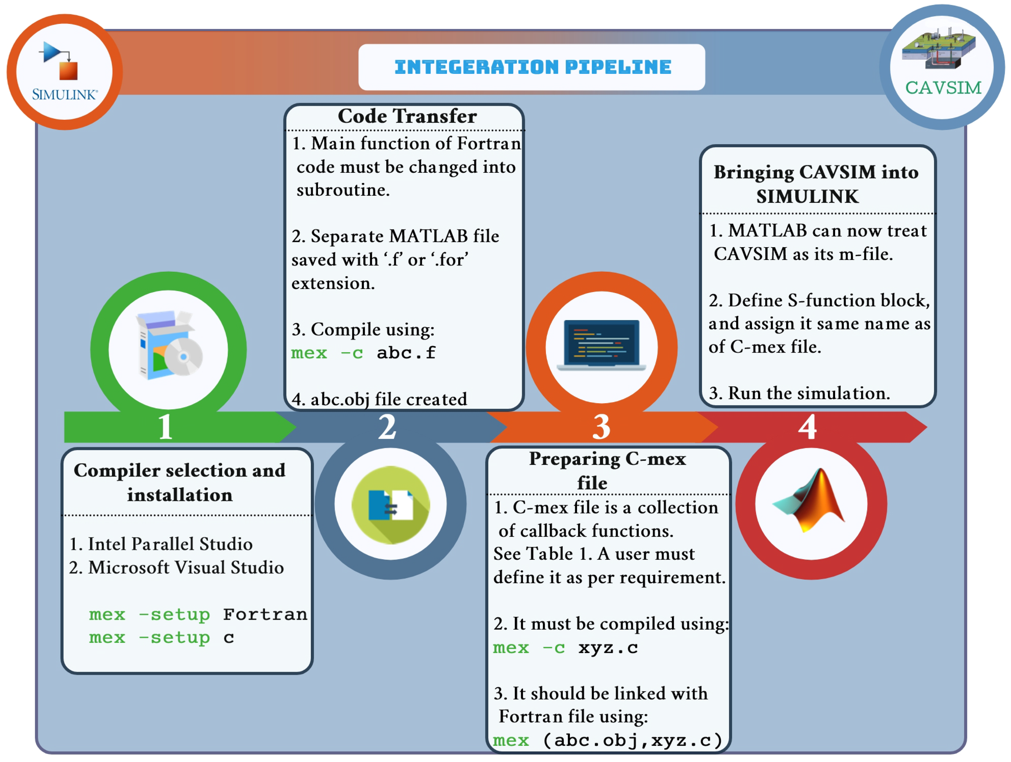
Compiler selection and Installation:

(a)

Two compilers need to be installed on the workstation:

i.

Intel parallel studio (IP) to compile FORTRAN files.

ii.

Microsoft visual studio (VS) to compile C/C++ files.

(b)

To make sure that compilers are correctly installed and detectable by MATLAB, use the following commands in the MATLAB command window:

mex -setup Fortran % detects the IP

mex -setup c % detects the VS

2.

Code Transfer:

(a)

Since MATLAB can only call FORTRAN’s subroutines, any main function in FORTRAN’s files must be changed into a subroutine. Any input/output variables that MATLAB needs to send or receive from FORTRAN must be declared as the functional parameters of that subroutine.

(b)

Every FORTRAN file must be transferred to a separate file in MATLAB’s editor and should either be saved as a ’.f ’ or ’.for’ extension.

(c)

Every ’.f’ or ’.for’ file transferred in MATLAB in 2b should be compiled using the following command in the MATLAB command window:

mex -c abc.f

i.

Where ’abc.f’ is the pseudonym of the FORTRAN file in MATLAB.

ii.

Additionally, ’c’ is the additional flag to force the compiler to only compile and not link with C-mex file; otherwise, MATLAB expects the name of C-mex file to be given.

iii.

Running the command in 2c should generate an ’abc.obj’ file that should have been saved in MATLAB’s working directory.

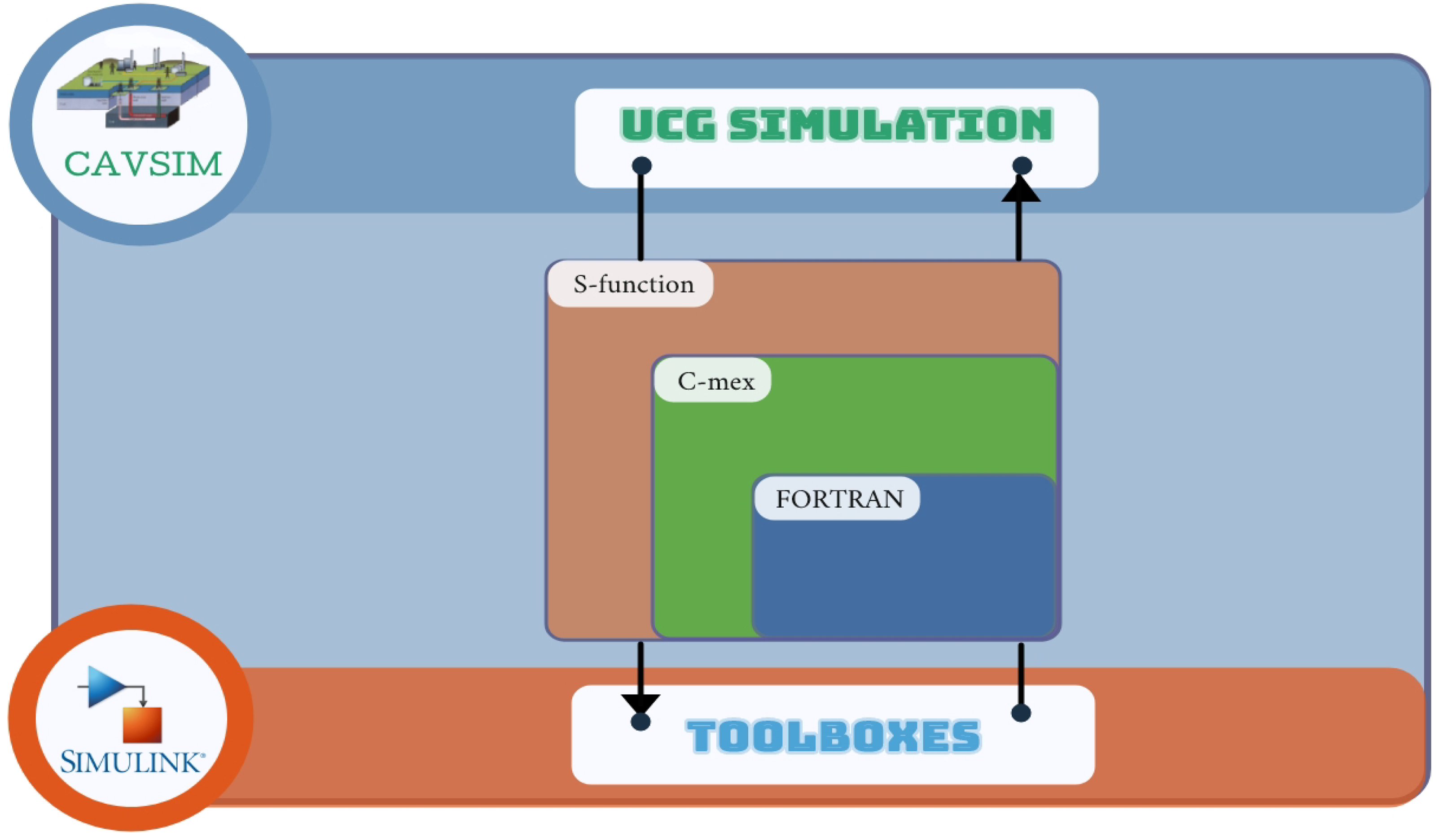
Once all the computational routines are successfully transferred and compiled, they need to be linked with the S-function via special gateway functions using ’.obj’ files.

3.

C-mex file preparation and compilation:

A C-mex file is a collection of callback functions that SIMULINK invokes at each simulation timestep.

Table 1. Important callback functions used by S-function.

Callback Function	Description
mdlInitializeSizes	Allocates the total number of input and output ports, their sizes, and other parameters of the S-function.
mdlInitializeSampleTimes	Specifies the time samples at which the S-function is invoked.
mdlOutputs	Calls and runs the FORTRAN computational subroutine.
mdlTerminate	Perform any actions required at termination of the simulation.

outlines the basic functionalities of the most important callback routines.

(a)

As gleaned from Table 1, the C-mex file should be edited according to the user’s specific needs, i.e., the total number of plant’s inputs and outputs, their sizes, and data types should be appropriately declared to avoid compatability issues.

(b)

Once the C-file has been prepared, it must be saved with a ’.c’ extension, i.e., ’xyz.c’, and compiled using the following command in MATLAB’s command window:

mex -c xyz.c

(c)

The ’abc.obj’ file generated in 2(c)iii is used to link the FORTRAN’s computational routines with the C-mex file compiled in 3b using the following command:

mex(abc.obj,xyz.c)

i.

If there is more than one FORTRAN computational routine, they can be compiled in a similar fashion using the following command:

mex(abc1.obj,abc2.obj,xyz.c)

Figure 6 summarises the steps taken to integrate CAVSIM with MATLAB.

4. Challenges and Solutions

The aim of this section is to present and generalise the challenges faced in this work. Moreover, any foreseen issues and their potential solutions are also introduced. Keeping in mind the methodology pipeline, the challenges are categorised into two types: pre- and post-integration.

4.1. Pre-Integration Challenges

The first and most trivial yet frequent issue that is bound to arise under such a type of integration is that of formatting. FORTRAN code, like most other programming languages, must adhere to a specific structure; failing to stick by those rules results in a compilation error. Since FORTRAN is not a free-format language, thus it imposes rigorous column position rules.

• Col. 1: Blank, or a ’c’ or ’*’ for comments.
• Col. 1–5: Statement label.
• Col. 6: Continuation of the previous line.
• Col. 7–72: Statement.
• Col. 73–80: Sequence number.

Therefore, in a situation where a bulk of code is being transferred to MATLAB’s editor via copy-pasting technique, care should be exercised that all the lines are landed on their respective columns. In the event of a compiler issuing the following error, which suggests a formatting issue, a user should simply indent back the block of code to its designated column. An interested reader may refer to the FORTRAN user manual for an exhaustive list of formatting instructions.

A partially similar and less frequent type of error is as follows:

“unrecognized error 5078 token”

Such an error type can be misleading as they have ambiguous sources. One possible cause is the presence of an unwanted ASCII character, which may have snuck into the code during code transfer. In such a case, a user may want to scan the binary file of the code to detect the presence of unwarranted ASCII characters. There are freely available online tools that can convert and scan the code file into its binary file.

Another possibility is anchored on the fact that modern versions of compilers are incompatible with older ones. For instance, in the earlier version, a programmer could concatenate two lines of code with the following combinations of ’/’ and ’&’ characters without passing additional instructions to the compiler.

format (/$‘$ This is line 1$’$\

&        /$‘$   This is line 2.$’$)

However, this is not possible in the later versions of the compiler since backslash edit descriptors are not enabled by default. To manually turn on such descriptors, additional flags need to be sent to the compiler. For the descriptor stated above, a program must be compiled using the following command:

mex -c COMPFLAGS=$‘$$COMPFLAGS -fpscomp:ioformat$’$ abc.f

For an additional list of flags and their description, see [45].

4.2. Post-integration Challenges

Even after successfully compiling and linking the program and defining it as an S-function block, errors may still crop up. Such errors are rather tricky to identify and tedious to rectify. This is due to the fact that MATLAB does not direct towards the error source and, in the worst-case scenario, comes crashing down without dispatching any warning.

Nonetheless, under these circumstances, the origin of the errors can be traced back to the following points: computational routine and C-mex. In the former case, either there is a presence of built-in libraries, internal functions, or computational routines that are not compatible with SIMULINK. In the latter, there might be a mismatch in the data types that are used by C-mex to link with FORTRAN, or, similarly, C-mex is not adequately defined according to the system parameters as illustrated in Section 3. Both of these issues and their proposed solutions are discussed in the following paragraphs.

FORTRAN has a bundle of built-in packages that are updated with each new release. However, the new compilers may not interrupt the old packages or libraries properly. As a consequence, a compiler does convert the program into an executable file; however, whilst running the code, garbage values are spawned due to the compiler’s un-interpretability. Unfortunately, under these conditions, there is no clear-cut way in MATLAB to locate the position in the program where garbage values are being introduced. However, the way out would be to write the input-output data in the text file wherever a sub-routine, function or library is invoked; and compare those variables against the standard program. Proceeding in this linear fashion, a user will ultimately ferret out the block of code, causing inconsistencies. As previously stated, when MATLAB is integrated with third-party software, the user is unable to interact with the program during run-time and receives no error messages. Therefore, unlike the error handling in their conventional software, MATLAB simply does not know how to react and proceed to shut down. This unnecessarily delays and hinders the debugging process. It is recommended that while in debugging mode, all the error-handling functions in the program be temporarily disabled and should be restored upon finishing the process.

There are a set of not-so-trivial errors or obstructions that may arise under special circumstances. This sub-section will briefly discuss them and offer solutions without indulging in details.

Missing Libraries

If the standard procedure for linking the FORTRAN routines and the C-mex gateway function, as illustrated in Figure 6 does not work, or if MATLAB issues the following error:

Error using mex

LINK: fatal error LNK1104: cannot open file $‘$ifconsol.lib$’$

This implies that VS is having trouble locating the library packages. To explicitly inform MATLAB of the libraries’ path, use the following command instead

fortranRoot = getenv( $‘$IFORTCOMPILERX$’$);

mex($‘$abc.F$’$, [$‘$-L$’$; fullfile(fortranRoot, $‘$compiler$’$,$‘$lib$’$, $‘$int el64win$’$) ]);

Where the variable IFORT COMPILERX is the system’s environment variable and points to the Intel Parallel Studio XE X root folder, which may vary from system to system, and X is the compiler’s version.

5. Post-Integration Processing

This section will focus on post-integration development, which was necessary to make CAVSIM completely autonomous from its environment—that is to say, that any control parameters can be edited directly in SIMULINK.

5.1. Asynchronous Clocks

The purpose was to make MATLAB a computational stage where it can run and manipulate the simulator’s outcome in run-time. Therefore, some tweaking was required before bringing in the controller. In this regard, the asynchronism in clocks had to be dealt with first. The following paragraph will highlight what asynchronism means in the context of current work and why it is necessary to remove it.

SIMULINK calls the S-function call-back functions at each of its time steps over the span of the complete simulation. However, at each instant when CAVSIM is invoked via the S-function, it does not give control back to SIMULINK until it has completed its own simulation. To illustrate, let $T_s$, $T_c$, $O\left(T_s\right)$ and $O\left(T_c\right)$ denote SIMULINK’s time, CAVSIM’s time, the S-function’s output at $T_s$, and CAVSIM’s output at $T_c$, respectively. At $T_s=0$, SIMULINK calls CAVSIM, which initialises the UCG simulation at $T_c=0$ and iterates it till $T_c$ becomes equal to the value defined by the user—let it be 3600 s—before relinquishing control back to SIMULINK. However, by that time, $T_c=3600$ s but $T_s=0$ s. This, in turn, implies that $\forall T_s,O\left(T_s\right)\ne O\left(T_c\right)$, indicating two asynchronous clocks running in loop. However, for the controller to be implemented in real-time, the output of the S-function at $T_s=0$ should be equal to the output of CAVSIM at $T_c=0$, i.e., $O\left(T_s\right)=O\left(T_c\right),\forall T_s$. Therefore, it was indispensable that CAVSIM’s clock be removed to accord it a controllable structure. Figure 7 demonstrates that at step 1 and $T_s=0$, SIMULINK makes a call to CAVSIM via the S-function interfaced through C-mex and gives control to CAVSIM, which initiates $T_c=0$. In step 2, the UCG simulation begins, and the value of $T_c$ starts incrementing to 3600 while $T_s$ remains constant. Finally, in step 3, upon ending the UCG simulation at $T_c=3600$, CAVSIM gives control back to SIMULINK via the same channel.

CAVSIM’s clock is a pseudo clock, i.e., it is not directly linked with the system’s clock. It is implemented by a computational routine embedded in a ‘for’ loop. However, since CAVSIM is a massive program spread over multiple files, finding the command incrementing the ‘for’ loop was a laborious task. It required scrutinising the values of variables after executing each command line. In this regard, the debugging feature of Power-station (PS)− a compiler for running CAVSIM− came in handy. It allows the user to inspect those values serially once the program has been compiled. The steps taken in Section 5.2 illustrate the process of attaching SIMULINK’s clock to CAVSIM along with further post-processing steps.

5.2. Input Output In-Dependency

The second step towards autonomy was to make CAVSIM parameters updatable, visually inspectable, and manipulatable directly from the SIMULINK without tinkering with CAVSIM. Steps illustrated in the following paragraph outline the whole post-prepossessing scheme, with Figure 8 giving the summary of those steps.

1.

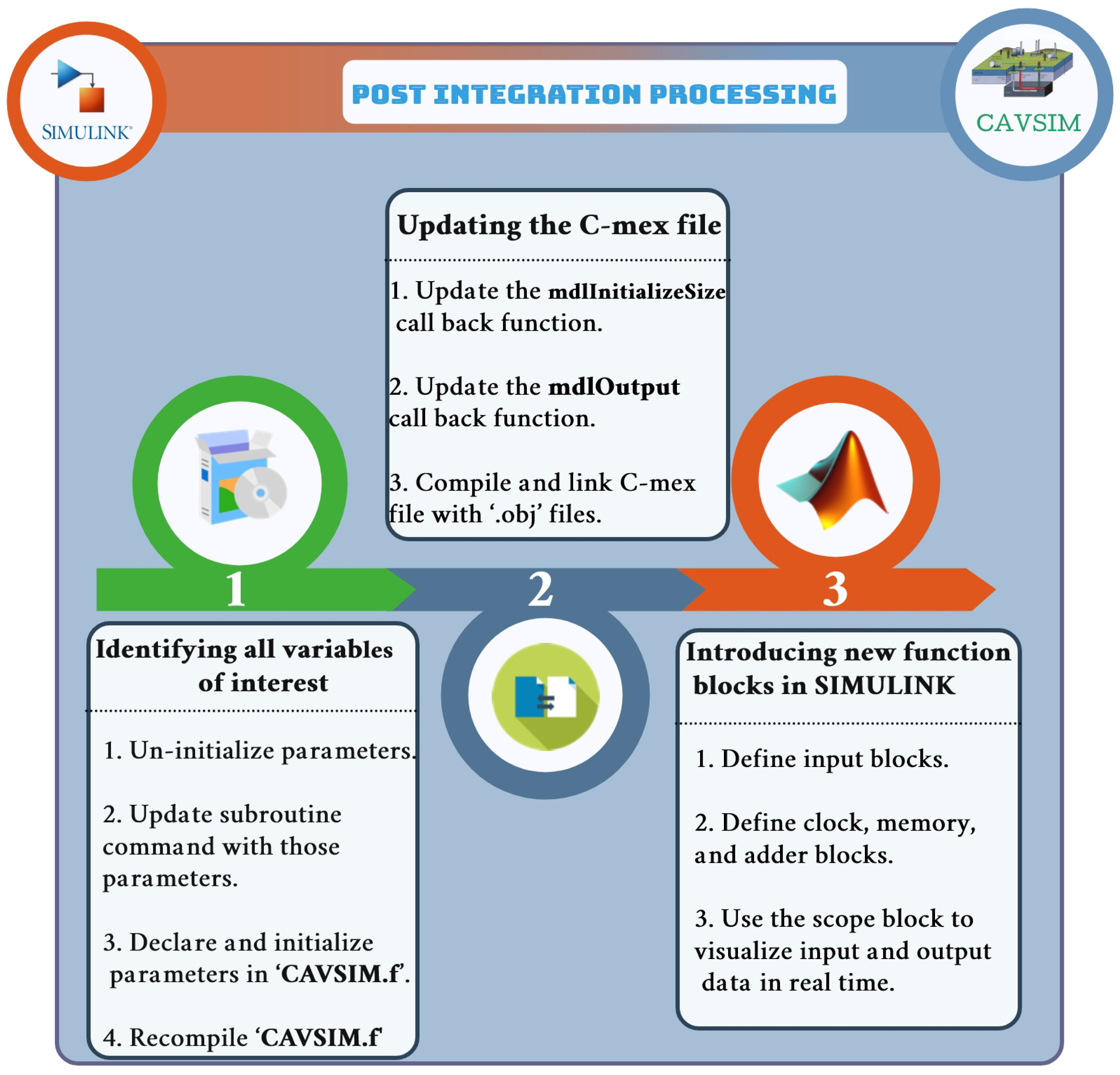
Identifying all the variables of interest:

(a)

This step involves (1) figuring out the parameterisable quantities that define the coal bed properties, process inputs, and outputs defined in CAVSIM; (2) locating their positions in the computational routine, and (3) initialising them. This step strips the CAVSIM of the capacity to initialise or update the variables from within.

(b)

Adding as many function parameters to the CAVSIM.f file’s subroutine command as the number of variables uninitialised in 1a. Doing so allows the user to give input to and retrieve output from CAVSIM using MATLAB.

(c)

Declaring new variables that are to be taken in from MATLAB via a subroutine command in the CAVSIM.f file

(d)

Re-initialising all the variables from 1a to the corresponding function parameters as newly defined in the subroutine command. This makes sure that all variables taken in now from MATLAB are mapped to their corresponding variables in CAVSIM.

(e)

Re-compiling the cavsim.f file as illustrated in 2c.

2.

Updating the C-mex file:

The following updates are necessary for the C-mex file to create a bi-directional channel for the data to be transferred between MATLAB and CAVSIM.

(a)

Updating the mdlInitializeSize call back function by declaring as many variables as identified in 1a. This step not only declares the new variables but also sets the data type, dimension, etc. Therefore, care must be exercised that all features defined here should be identical to 1d to avoid compatibility issues.

(b)

Updating the mdlOutput callback function by introducing as many variables as identified in 1a. This is a callback method that calls the main subroutine whilst transferring the input and output data.

(c)

Compiling and linking the newly updated C-mex file with all other ”.obj” files as illustrated in 3. This results in the upgrading of the S-function block with the associated input and output ports. The order of the input and the output channels of the S-function block is similar to the order of the variables defined in the C-mex and CAVSIM.f files, which must be the same as well.

3.

Introducing new function blocks in SIMULINK:

The previous steps taken have developed the desired interface between CAVSIM and MATLAB through which data from MATLAB can be mapped onto the corresponding variables in CAVSIM. However, for plant parameters to be directly updatable from SIMULINK, some additional blocks need to be introduced.

(a)

Define input blocks

i

The input can either be generated using SIMULINK’s source block or be imported from the workspace as a MATLAB timeseries object.

(b)

Define clock, memory, and adder blocks to give simulation time and time-step information from SIMULINK.

(c)

Use the scope block to visualise input and output data in real time.

(d)

Attach all these blocks to their respective ports of S-function as identified in 2c.

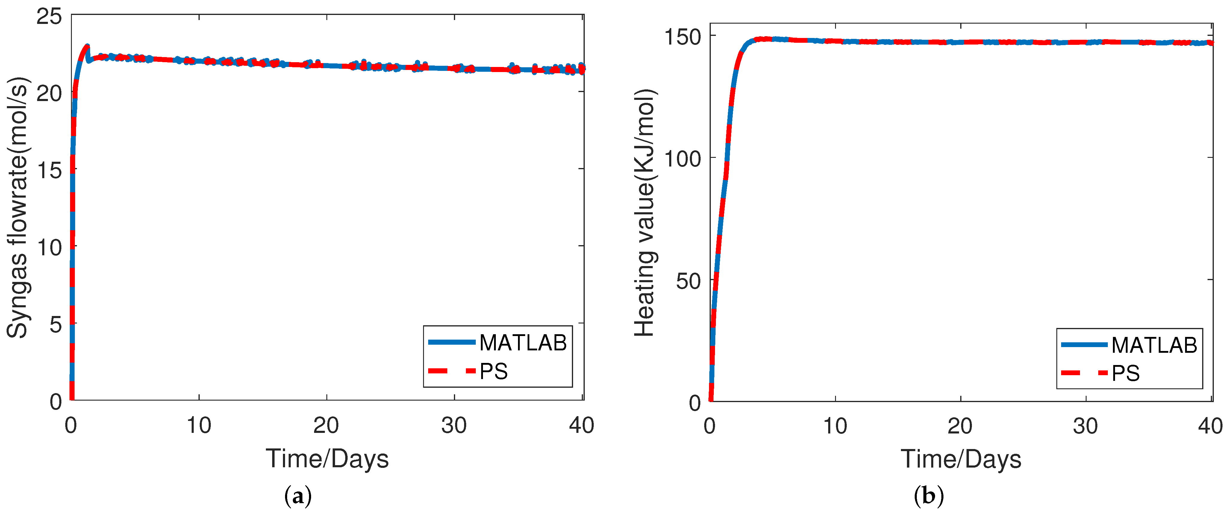
All in all, exercising the above yielded the desired controllable structure of CAVSIM in MATLAB. Upon these modifications, any process and parametrisable variables previously defined in CAVSIM are now updateable from MATLAB. Furthermore, turning off CAVSIM’s clock allows the user to access, visualise, and manipulate the plant’s output at each iteration of the simulation, thereby completing the development phase of CAVSIM into CAVLAB. Figure 9 represents the block-diagram, controllable structure of CAVLAB, wherein the user can either give built-in SIMULINK functions or custom-made MATLAB functions as input to the UCG system; similarly, the ’dt’ block allows the user to define the step-size information for the numerical solver; moreover, attaching the scope allows the user to perceive the simulation’s results in run-time. Moreover,

Table 2. Pre-integration and post-integration challenges.

Pre-Integration Challenges	Post-Integration Challenges	Remarks
Choosing the right MATLAB API to interface with FORTRAN subroutines	Optimising the performance and accuracy of the integration	Different MATLAB APIs have varying pros and cons depending on the problem type and complexity. For instance, the FORTRAN MEX API enables FORTRAN subroutines to be accessed by MATLAB functions, while the FORTRAN Engine API allows running and evaluating MATLAB functions from FORTRAN programs.
Writing a MEX file to call FORTRAN routines from MATLAB	Debugging and testing the integrated code	Creating a MEX file involves adhering to some specific rules and conventions for compiling and linking the FORTRAN code with MATLAB. External tools or libraries, such as gdb or f2py, may be needed for debugging and testing the integrated code.
Converting MATLAB data types to FORTRAN data types	Updating and maintaining the code for compatibility and functionality	MATLAB and FORTRAN differ in data types and memory layouts, which may lead to errors or inefficiencies if not managed properly. For instance, MATLAB uses column-major order for matrices, while FORTRAN uses row-major order. The code may need to be updated and maintained according to changes in MATLAB or FORTRAN versions, libraries, or platforms.
Learning the syntax and features of FORTRAN	Comparing the advantages and disadvantages of MATLAB and FORTRAN	FORTRAN is a lower-level language than MATLAB, which may offer more control over memory management, data structures, loops, etc. However, it may also lack built-in functions, libraries, or tools for matrix computations, symbolic manipulations, or visualisation.
Finding reliable and compatible FORTRAN libraries or routines	Dealing with potential errors or bugs in FORTRAN libraries or routines	FORTRAN has a long history and legacy of numerical software development, which means there may be many available libraries or routines for various problems. However, some of them may be outdated, incompatible, or poorly documented. Some of them may also have errors or bugs that are hard to detect or fix.

provides a comprehensive summary of important pre- and post-integration challenges that occurred in methodology pipeline.

6. CAVLAB Testing

Due to differences in data-handling capabilities, such as floating point precision, and incompatibility among data types of MATLAB and FORTRAN, the same computational routine may yield different results, as demonstrated by [46]. Therefore, to make sure that the CAVLAB and CAVSIM yield the same result in their respective environments, comparing their outputs under the same setting was imperative. In spite of the availability of a range of variables, the geometry of the cavity [8], which is the cumulative outcome of all the varying underlying processes, was selected as one of the process variables, with others being the heating value and flowrate of syngas for comparison and validation. A final check was performed to ensure that both computing environments were functioning under identical conditions; inputs, total simulation time, step size, and other variables were all set to the same values.

Both plants were run for a total simulation time of 40 days, with a step-size of 1 h, enough time for the reactor to execute important dynamics, and the output variables from CAVSIM were copied to an Excel sheet. An m-file, which was written in advance to read the CSV file and plot the geometry, generated the plots.

Table 3. Inputs and Outputs of the UCG plant.

Plant Inputs	Plant Outputs
Steam to oxygen ratio $({\mathrm{H}}_2\mathrm{O}/{\mathrm{O}}_2)$	Heating value (KJ/mol)
Inlet gas flowrate (mol/s)	Flowrate (mol/s)

highlights the inputs and outputs against which both software are validated.

Figure 10a,b shows the cavity’s shape as it was predicted by MATLAB and PS on days 20 and 35, respectively. As expected, as the days go by, the cavity moves upwardly towards the overburden, and the shapes predicted by the two simulation environments for different days conform with one another, demonstrating that both software packages handled computation similarly.

Similarly, Figure 11a,b shows the flowrate and heating value, respectively, as simulated by CAVSIM and CAVLAB for the following values of the input: Table 3. It can be observed that for the total span of the simulation, the simulated outputs by both packages yield the same numeric values. Likewise, both simulators exhibited the same consistent behaviour across various inputs, parameters, and numeric conditions, indicating successful integration: a standardized procedure of validation for such scenarios [47,48].

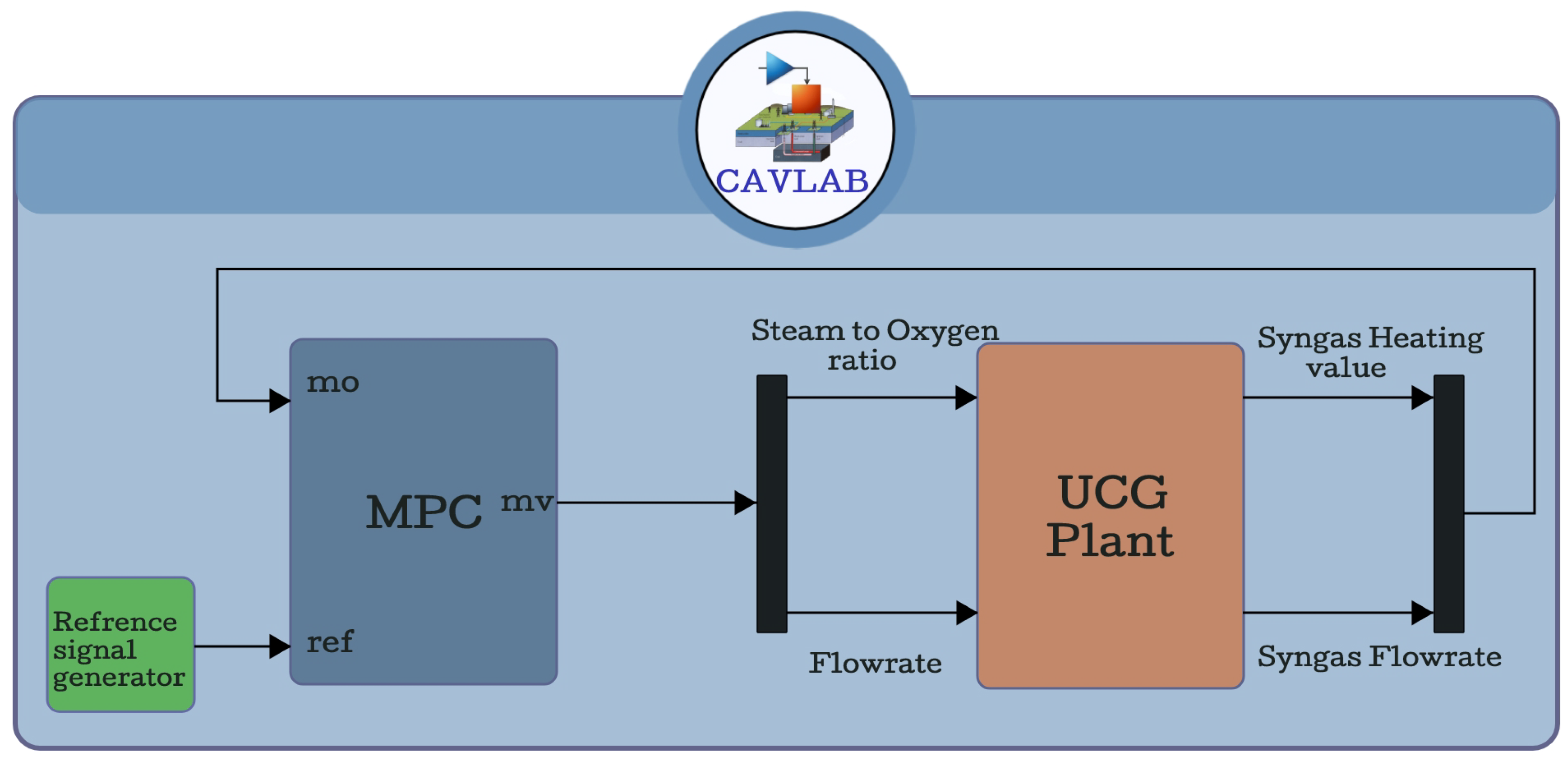
7. Case Study: MPC Design for UCG Plant Using MATLAB’s Toolbox

Affording CAVSIM a controllable structure in MATLAB implies that it can now exploit all of the latter’s toolboxes. In this case study, a demonstration of one of the design aspects of the UCG process is provided: synthesising an optimal controller using MATLAB’s MPC toolbox. In this section, a brief introduction of MPC is provided that is followed by an illustrative procedure of its design and deployment on CAVSIM, and consequently, the results of the plant’s and controller’s outputs are provided.

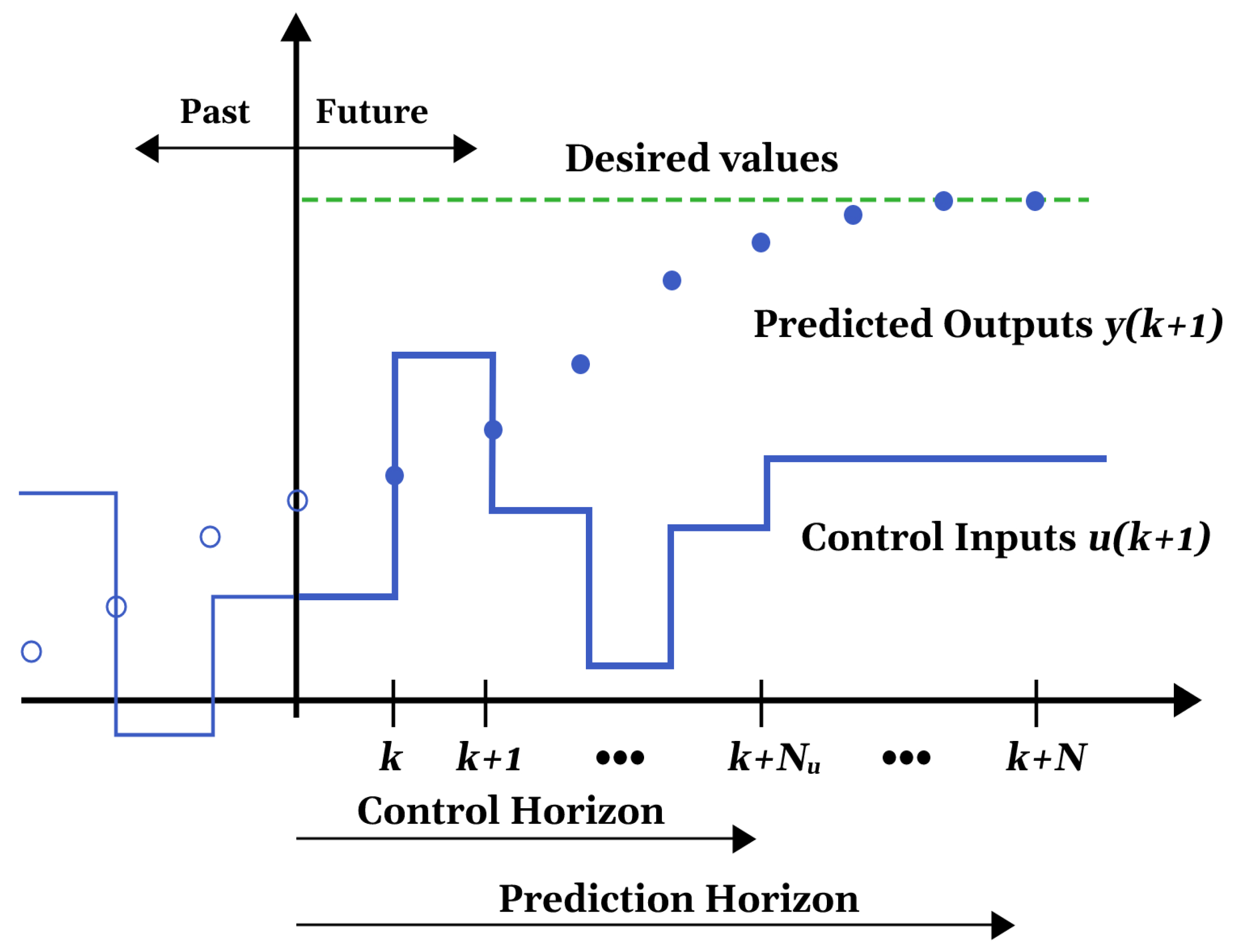
7.1. MPC Problem Formulation

MPC gained momentum in the 1970s, with a particular interest in chemical-based industry processes. These processes have operational constraints in terms of inputs, outputs, and states, such as valve saturation or temperature of a catalyst. Therefrom, MPC has widely been adopted for complex multi-variables industrial scaled processes that have constraints in them [49].

MPC is an optimal control strategy that generates a set of optimal control steps based on the system’s and controller’s current output [50]. MPC achieves this by using a plant model to predict the plant’s output for some p points into the future, where $T_p$ is known as prediction horizon. The plant, coupled with an optimiser generates a set of optimal controller outputs for some points ch into the future; where $T_{ch}$ is known as the control horizon, and $T_{ch}\le T_p$ generally—see Figure 12. The optimiser achieves the desired results by solving the following optimisation problem:

$$\begin{array}{cc}\hfill & \underset{{\mathit{u}}_{\mathit{0}},{\mathit{u}}_{\mathit{1}},...,{\mathit{u}}_{\mathit{N}-\mathit{1}}}{min}J=\sum _{k=0}^{N-1}\left({{\mathit{x}}_{\mathit{k}}}^T\mathit{Q}{\mathit{x}}_{\mathit{k}}+{{\mathit{u}}_{\mathit{k}}}^T\mathit{R}{\mathit{u}}_{\mathit{k}}\right)+{{\mathit{x}}_{\mathit{N}}}^T\mathit{P}{\mathit{x}}_{\mathit{N}},\hfill \\ \hfill & \mathrm{subject}\mathrm{to}:\hfill \\ \hfill & {\mathit{x}}_{\mathit{0}}={\mathit{x}}_{\mathrm{current}},\hfill \\ \hfill & {\mathit{x}}_{\mathit{k}+\mathit{1}}=\mathit{A}{\mathit{x}}_{\mathit{k}}+\mathit{B}{\mathit{u}}_{\mathit{k}},\hfill \\ \hfill & {\mathit{x}}_{\mathit{k}}\in \mathcal{X},\hfill \\ \hfill & {\mathit{u}}_{\mathit{k}}\in \mathcal{U},\hfill \\ \hfill & k=0,1,...,N-1,\hfill \end{array}$$

where ${\mathit{x}}_{\mathit{k}}$ and ${\mathit{u}}_{\mathit{k}}$ are predicted state and input, respectively, at time step k. $\mathit{A}$ is the system matrix, and $\mathit{B}$ is the input matrix that relates the inputs to the states. At the same time, $\mathit{Q}$, $\mathit{R}$, and $\mathit{S}$ are weighting matrices for states, inputs, and terminal states, respectively, to penalise them. $\mathcal{X}$ and $\mathcal{U}$ are set of constraints on states and inputs, and N is the prediction horizon.

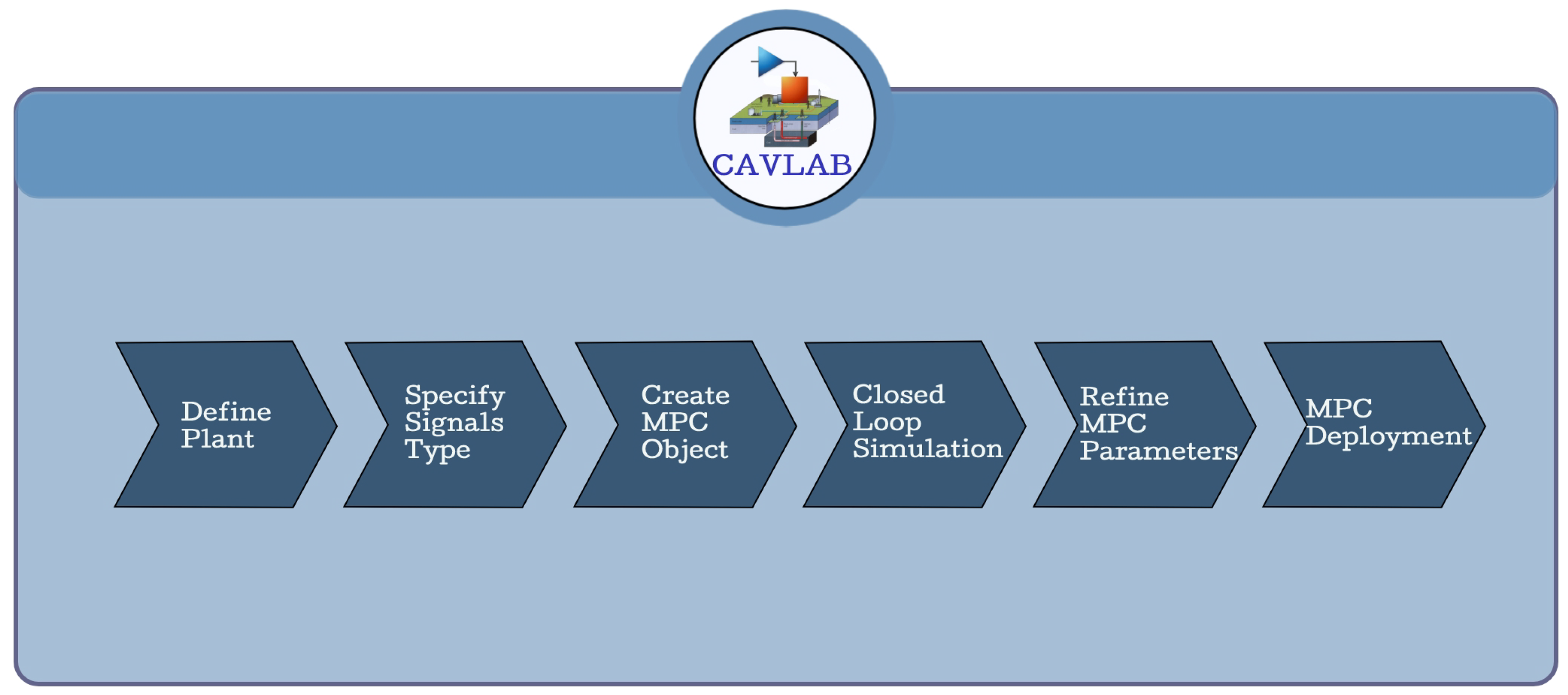
7.2. MPC Implementation

This study considers a data-driven Multiple Input Multiple Output, Non-linear Autoregressive with Exogenous Inputs model for UCG, previously derived in our work- which, at the time of writing, is under submission wherein the inputs and outputs are taken the same as given by Table 3. The task of the controller is to track the desired trajectory under actuator constraints. Figure 13 shows the schematic of the UCG plant with MPC as implemented in MATLAB.

The design steps to synthesise and implement an MPC in MATLAB are given in Figure 14 and are listed below:

1.

The first step in designing an MPC controller in MATLAB is to define the plant, which is the mathematical model of the system that is to be controlled. This can be done by creating a SIMULINK model or using system identification techniques to obtain a mathematical model from input-output data. The plant model should capture the dynamic behaviour of the system to be controlled.

2.

The second step is to specify the type of input signals that will be used in the MPC controller, such as setpoints, disturbances, and measured outputs.

3.

This step involves defining the prediction and control horizons, constraints on the input and output signals, and the cost function.

4.

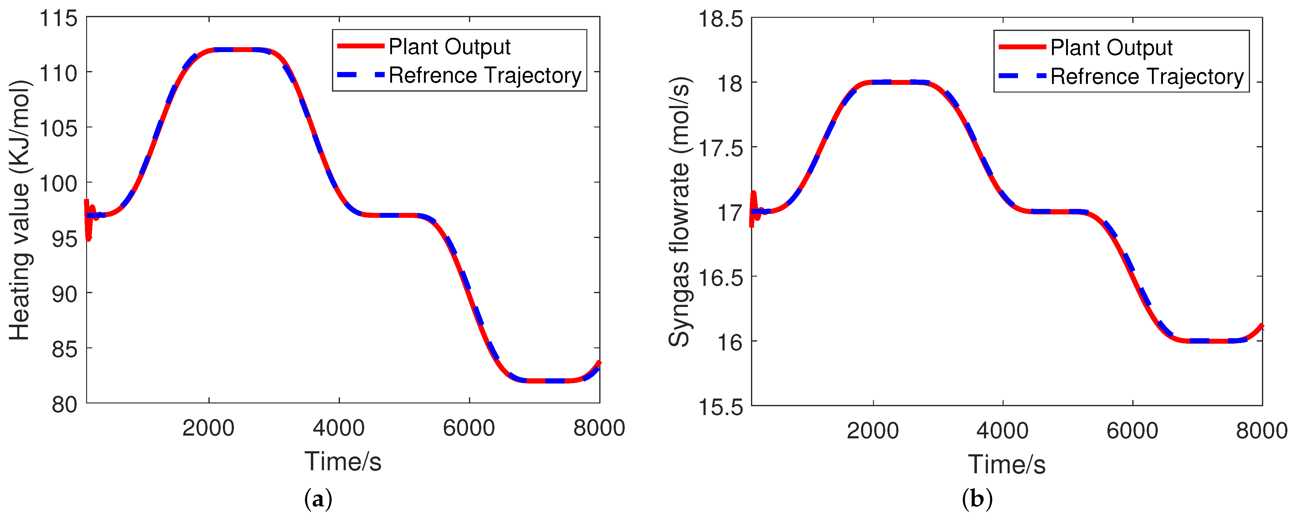
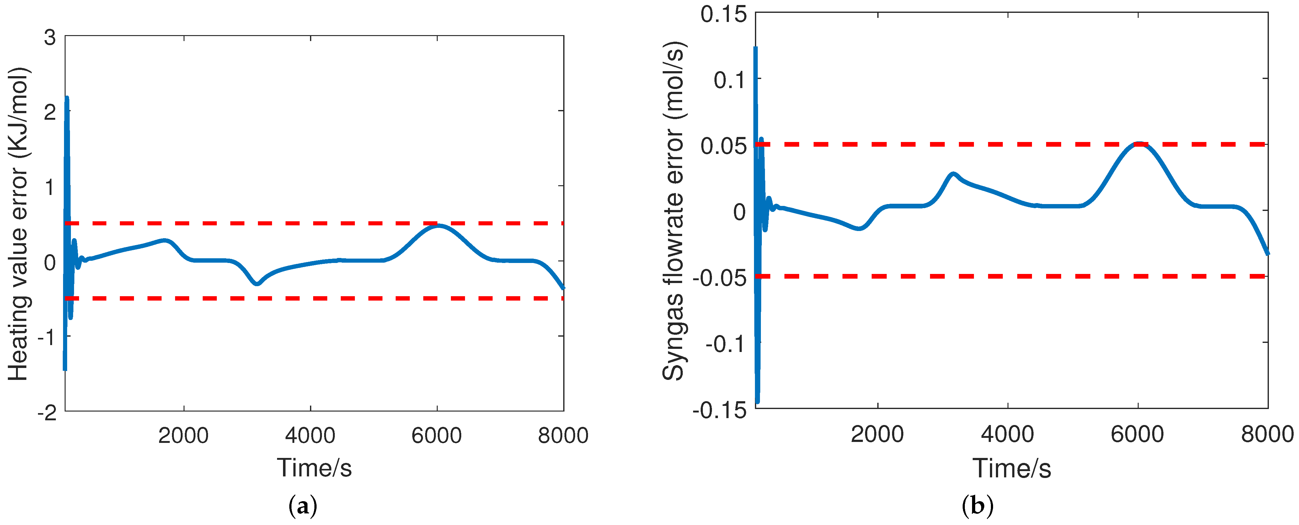
Once the MPC object is created, a closed-loop simulation is performed to evaluate the performance of the MPC controller. This involves simulating the system’s response to different input signals and comparing it with the desired response.

5.

This step involves adjusting the tuning parameters of the MPC controller, such as the weights in the cost function and the prediction horizon. The simulation results are used to evaluate the controller’s performance, and the tuning parameters are adjusted iteratively until the desired performance is achieved.

6.

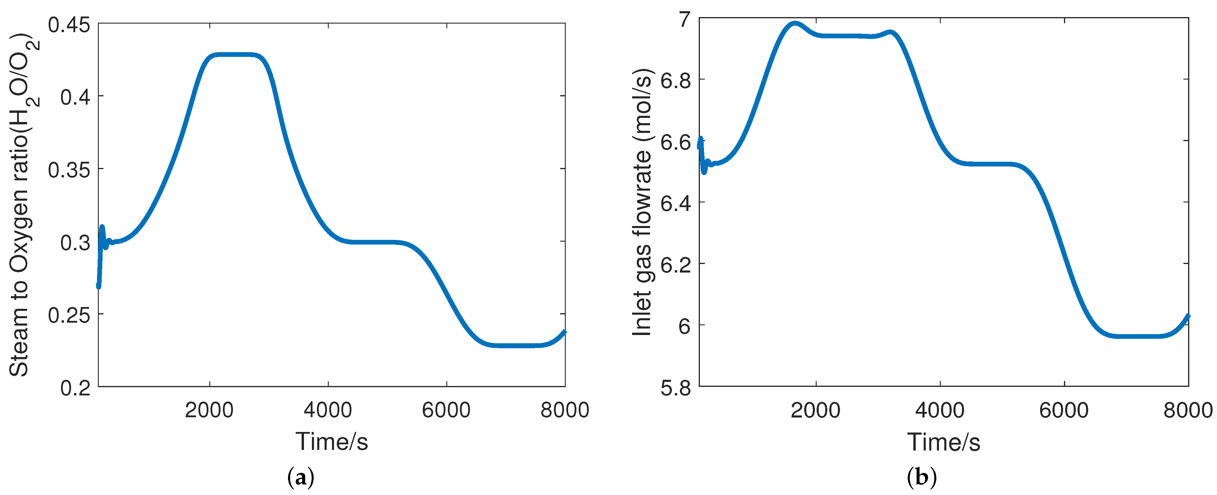
The controller takes measurements from the plant model and calculates the control inputs that optimize the system’s performance. The simulation results are used to evaluate the controller’s performance, and the tuning parameters are adjusted if necessary to maintain optimal performance.

Figure 15a,b show the graphs of the desired trajectory and the actual outputs of the heating value, and flowrate, respectively; similarly, Figure 16a,b show the graphs of tracking errors for heating value and flowrate, respectively. Moreover, Figure 17a,b shows the controller’s output for each input of the UCG plant. The statistical metrics to quantify the controller’s performance are Mean Absolute Error (MAE), Root Mean Square Error (RMSE), and Controller Effort (CE) and are defined in

Table 4. Performance measures and criteria.

Tool	Formulas	Values
RMSE	$\sqrt{\frac{1}{n}{\sum }_{i=1}^n{(r_i-y_i)}^2}$	heating value = 0.23 flowrate = 0.02
MAE	$\frac{1}{n}{\sum }_{i=1}^n|r_i-y_i|$	heating value = 0.13 flowrate = 0.012
CE	${\parallel u\parallel }_2=\sqrt{{\sum }_{i=1}^n{u}_i^2}$	heating value = 28.48 flowrate = 580.26

along with their values against respected outputs.

A closer inspection of Figure 15a,b reveals that the maximum deviation of the plant’s output—heating value, and flowrate—are 2.17 KJ/mol and −0.15 mol/s, respectively; moreover, apart from the initial discrepancy, the tracking errors are within the bounds of ±0.5 KJ/mol and ±0.05 mol/s for heating value and flowrate, respectively. Similarly, the MAE and RMSE scores demonstrate a good performance of the controller in terms of tracking.

8. Extension in Research Scope of UCG

The controller design is one of the determining factors underlying the operational feasibility of any UCG plant. Moreover, the integration of CAVSIM with MATLAB opens up the opportunity to analyse different design scenarios, as illustrated in the following sub-sections. However, it is worth emphasising that no single simulator can encapsulate all aspects of nature due to obvious constraints in computational resources and mathematical analysis [51]. In this respect, CAVLAB is no exception; for instance, the STARS module of the Computer Modelling Group (CMG) offers additional features such as geological structure, porosity/permeability variation, etc. [52]. On the same grounds, Cav3d [42] has more capabilities than CAVLAB in modelling cavity evolution and growth during UCG. Although CAVLAB simplifies the wall and roof surface growth and assumes an axisymmetric cavity shape, Cav3d accounts for the thermo-mechanical failure of coal and rock and the effects of complex cavity shapes, heterogeneous coal seams, and dynamic gas source locations on the gasification process. Similarly, the CFD-based models can also predict the cavity growth of small-core gasification [53,54]. However, implementing these models requires expertise in specific software such as ANSYS, COMSOL-MULTIPHYSICS, etc., which is time-consuming and computationally more expensive [55] than CAVLAB.

8.1. Optimal Resource Utilisation

For any given UCG reactor, the amount of coal has some fixed value, which implies that only as much of the syngas’ heating value can be recovered from the reactor’s natural lifespan. However, due to chemical kinetics and other structural phenomena such as cavity development and roof rubblisation, not all of the coal is utilised as the reactor draws near its end, thus indicating the residual heating value that could potentially have been relinquished. It turns out that if the reactor is driven in a certain trajectory along its dynamics, maximum coal, thus maximum heating value, can be recovered. Since the plant’s input is the only control we have at our disposal to drive the reactor, the problem of optimal resource utilisation can be formulated as finding the optimal input trajectory such that the yield of heating value is maximised. Thus, an optimal input can be found by parametrising the input functions using Fourier decomposition, and optimal Fourier coefficients can be searched using metaheuristic search techniques such as genetic algorithms. In this respect, MATLAB has built-in functions that help users conveniently formulate and solve optimisation problems.

8.2. Data-Driven Modelling

The paradigm of mathematical modelling lies on a continuous spectrum, with first-principle models on one extreme and data-driven models on the other. Regarding the latter approach, it is a principled procedure for determining a mathematical map between a set of inputs and outputs for any system. Data-driven modelling is an active research area for any general dynamical system. However, unlike the first-principle-based modelling of the UCG, which abounds in the literature, data-driven or system identification is still in the seminal stage. This, we believe, is largely due to the lack of a generalised framework wherein all the steps of the system identification procedure can be carried out. Due to the integrated structure of CAVLAB, the design of experiments (DoE) in system identification, which constitutes model selection and synthesis of the excitation signal, collecting simulation data, and training and validating the identified model, can all be done in the same software, thus making the whole process streamlined and efficient.

9. Conclusions

CAVSIM is a standalone UCG process software package that can simulate the cavity growth of a parametrisable coal reactor. CAVSIM is integrated with MATLAB to benefit from its superior data-handling capabilities, built-in toolboxes, and ease of visualisation. Additionally, a thorough discussion of the integration’s underlying process and methodology is provided. Moreover, the results of the simulation of a UCG process for different operating conditions in both software are shown, which demonstrate identical behaviour. Lastly, a walk-through of the user operation of CAVLAB has also been touched upon.

CAVLAB extends the scope of its preceding version by putting forth the UCG system in a controllable structure, wherein the user has the autonomy of parameterising the plant against the diversified set of UCG reactors across the globe; the flexibility of designing custom-defined inputs; the advantage of visualising the plant’s output whilst the simulation is running; and accessibility to the full range of built-in toolboxes of MATLAB. All of these added functionalities were demonstrated in a case study wherein an MPC controller was designed for a UCG plant. In the same vein, the applications of other research areas for UCG as a consequence of integration have also been discussed.

Computer code availability

The simulator is available as a SIMULINK/MATLAB file under an MIT license.

• Name of simulator: CAVLAB.slx
• Software used: MATLAB 2019b
• Availability: The whole package, along with instructions, is available at github (accessed on 1 March 2023): https://github.com/Hilberto-inf/CAVLAB–UCG-process-simulator.

References

1. Jiang, L.; Chen, S.; Chen, Y.; Chen, Z.; Sun, F.; Dong, X.; Wu, K. Underground coal gasification modelling in deep coal seams and its implications to carbon storage in a climate-conscious world. Fuel 2023, 332, 126016. [Google Scholar] [CrossRef]
2. Klebingat, S.; Kempka, T.; Schulten, M.; Azzam, R.; Fernández-Steeger, T.M. Innovative thermodynamic underground coal gasification model for coupled synthesis gas quality and tar production analyses. Fuel 2016, 183, 680–686. [Google Scholar] [CrossRef]
3. Ammarullah, M.I.; Hartono, R.; Supriyono, T.; Santoso, G.; Sugiharto, S.; Permana, M.S. Polycrystalline Diamond as a Potential Material for the Hard-on-Hard Bearing of Total Hip Prosthesis: Von Mises Stress Analysis. Biomedicines 2023, 11, 951. [Google Scholar] [CrossRef] [PubMed]
4. Ammarullah, M.I.; Santoso, G.; Sugiharto, S.; Supriyono, T.; Wibowo, D.B.; Kurdi, O.; Tauviqirrahman, M.; Jamari, J. Minimizing Risk of Failure from Ceramic-on-Ceramic Total Hip Prosthesis by Selecting Ceramic Materials Based on Tresca Stress. Sustainability 2022, 14, 13413. [Google Scholar] [CrossRef]
5. Ammarullah, M.I.; Afif, I.Y.; Maula, M.I.; Winarni, T.I.; Tauviqirrahman, M.; Akbar, I.; Basri, H.; van der Heide, E.; Jamari, J. Tresca Stress Simulation of Metal-on-Metal Total Hip Arthroplasty during Normal Walking Activity. Materials 2021, 14, 7554. [Google Scholar] [CrossRef]
6. Xu, H.; Li, X.; Li, Y.; Meng, D.; Wang, X. Stiffness Modeling and Dynamics Co-Modeling for Space Cable-Driven Linkage Continuous Manipulators. Mathematics 2023, 11, 1874. [Google Scholar] [CrossRef]
7. Thorsness, C.B.; Britten, J.A. CAVISM User Manual. 1989. Available online: https://doi.org/10.2172/6307133 (accessed on 27 April 2023).
8. Javed, S.B.; Uppal, A.A.; Bhatti, A.I.; Samar, R. Prediction and parametric analysis of cavity growth for the underground coal gasification project Thar. Energy 2019, 172, 1277–1290. [Google Scholar] [CrossRef]
9. Javed, S.B. Cavity Prediction and Multi-variable Control of Underground Coal Gasification Process. Ph.D. Thesis, Capital University of Science and Technology, Islamabad. Available online: https://cust.edu.pk/static/uploads/2021/09/PhD-EE-Thesis-Syed-Bilal-Javed.pdf (accessed on 24 May 2023).
10. Javed, S.B.; Uppal, A.A.; Samar, R.; Bhatti, A.I. Design and implementation of multi-variable H robust control for the underground coal gasification project Thar. Energy 2021, 216, 119000. [Google Scholar] [CrossRef]
11. Javed, S.B.; Utkin, V.I.; Uppal, A.A.; Samar, R.; Bhatti, A.I. Data-Driven Modeling and Design of Multivariable Dynamic Sliding Mode Control for the Underground Coal Gasification Project Thar. IEEE Trans. Control Syst. Technol. 2021, 30, 153–165. [Google Scholar] [CrossRef]
12. Prakoso, A.T.; Basri, H.; Adanta, D.; Yani, I.; Ammarullah, M.I.; Akbar, I.; Ghazali, F.A.; Syahrom, A.; Kamarul, T. The Effect of Tortuosity on Permeability of Porous Scaffold. Biomedicines 2023, 11, 427. [Google Scholar] [CrossRef]
13. Jamari, J.; Ammarullah, M.I.; Santoso, G.; Sugiharto, S.; Supriyono, T.; Permana, M.S.; Winarni, T.I.; van der Heide, E. Adopted walking condition for computational simulation approach on bearing of hip joint prosthesis: Review over the past 30 years. Heliyon 2022, 8, e12050. [Google Scholar] [CrossRef] [PubMed]
14. Thorsness, C.B.; Rozsa, R.B. In-Situ Coal Gasification: Model Calculations and Laboratory Experiments. SPE J. 1978, 18, 105–116. [Google Scholar] [CrossRef]
15. Abdel-Hadi, E.A.A.; Hsu, T.R. Computer Modeling of Fixed Bed Underground Coal Gasification Using the Permeation Method. J. Energy Res. Technol. 1987, 109, 11–20. [Google Scholar] [CrossRef]
16. Uppal, A.A.; Bhatti, A.I.; Aamir, E.; Samar, R.; Khan, S.A. Control oriented modeling and optimization of one dimensional packed bed model of underground coal gasification. J. Process Control 2014, 24, 269–277. [Google Scholar] [CrossRef]
17. Żogała, A. Critical Analysis of Underground Coal Gasification Models. Part I: Equilibrium Models – Literary Studies. J. Sustain. Min. 2014, 13, 22–28. [Google Scholar] [CrossRef]
18. Perkins, G.; Sahajwalla, V. Steady-State Model for Estimating Gas Production from Underground Coal Gasification. Energy Fuels 2008, 22, 3902–3914. [Google Scholar] [CrossRef]
19. 2009. Available online: https://www.cfd.com.au/cfd_conf09/PDFs/196LUO.pdf (accessed on 2 September 2022).
20. Seifi, M.; Abedi, J.; Chen, Z. The Analytical Modeling of Underground Coal Gasification through the Application of a Channel Method. Energy Sources Part A 2013, 35, 1717–1727. [Google Scholar] [CrossRef]
21. Massaquoi, J.G.M.; Riggs, J.B. Mathematical modeling of combustion and gasification of a wet coal slab—I: Model development and verification. Chem. Eng. Sci. 1983, 38, 1747–1756. [Google Scholar] [CrossRef]
22. Perkins, G.; Sahajwalla, V. A Mathematical Model for the Chemical Reaction of a Semi-infinite Block of Coal in Underground Coal Gasification. Energy Fuels 2005, 19, 1679–1692. [Google Scholar] [CrossRef]
23. Samdani, G.; Aghalayam, P.; Ganesh, A.; Sapru, R.K.; Lohar, B.L.; Mahajani, S. A process model for underground coal gasification—Part-II growth of outflow channel. Fuel 2016, 181, 587–599. [Google Scholar] [CrossRef]
24. Biezen, E.N.J.; Bruining, J.; Molenaar, J. An Integrated 3D Model for Underground Coal Gasification. In Proceedings of the SPE Annual Technical Conference and Exhibition, Dallas, TX, USA, 22 October 1995. [Google Scholar] [CrossRef]
25. Nitao, J.J.; Buscheck, T.A.; Ezzedine, S.M.; Friedmann, S.J.; Camp, D.W. An Integrated 3-D UCG Model for Predicting Cavity Growth, Product Gas, and Interactions with the Host Environment. 2017. Available online: https://www.osti.gov/servlets/purl/1573942 (accessed on 27 April 2023).
26. Hasse, C.; Debiagi, P.; Wen, X.; Hildebrandt, K.; Vascellari, M.; Faravelli, T. Advanced modeling approaches for CFD simulations of coal combustion and gasification. Prog. Energy Combust. Sci. 2021, 86, 100938. [Google Scholar] [CrossRef]
27. Tauviqirrahman, M.; Jamari, J.; Susilowati, S.; Pujiastuti, C.; Setiyana, B.; Pasaribu, A.H.; Ammarullah, M.I. Performance Comparison of Newtonian and Non-Newtonian Fluid on a Heterogeneous Slip/No-Slip Journal Bearing System Based on CFD-FSI Method. Fluids 2022, 7, 225. [Google Scholar] [CrossRef]
28. Putra, R.U.; Basri, H.; Prakoso, A.T.; Chandra, H.; Ammarullah, M.I.; Akbar, I.; Syahrom, A.; Kamarul, T. Level of Activity Changes Increases the Fatigue Life of the Porous Magnesium Scaffold, as Observed in Dynamic Immersion Tests, over Time. Sustainability 2023, 15, 823. [Google Scholar] [CrossRef]
29. Mahseredjian, J.; Benmouyal, G.; Lombard, X.; Zouiti, M.; Bressac, B.; Gerin-Lajoie, L. A link between EMTP and MATLAB for user-defined modeling. IEEE Trans. Power Deliv. 1998, 13, 667–674. [Google Scholar] [CrossRef]
30. Ahsan, M.; Saramaki, T. Significant improvements in translating the Parks-McClellan Algorithm from its FORTRAN code to its corresponding MATLAB code. In Proceedings of the 2009 IEEE International Symposium on Circuits and Systems, Taipei, Taiwan, 24–27 May 2009; pp. 289–292. [Google Scholar] [CrossRef]
31. Bagal, K.; Kadu, C.; Parvat, B.; Vikhe, P. PLC Based Real Time Process Control Using SCADA and MATLAB. In Proceedings of the 2018 Fourth International Conference on Computing Communication Control and Automation (ICCUBEA), Pune, India, 16–18 August 2018; pp. 1–5. [Google Scholar] [CrossRef]
32. Ivan, G.; Nikolay, S.; Vladislav, L.; Andrei, P. Solving of Mathematical Problems in the C# Based on Integration with MATLAB. In Proceedings of the 2020 Ural Symposium on Biomedical Engineering, Radioelectronics and Information Technology (USBEREIT), Yekaterinburg, Russia, 14–15 May 2020; pp. 432–435. [Google Scholar] [CrossRef]
33. Sokos, E.N.; Zahradnik, J. ISOLA a Fortran code and a Matlab GUI to perform multiple-point source inversion of seismic data. Comput. Geosci. 2008, 34, 967–977. [Google Scholar] [CrossRef]
34. Andersson, C.; Führer, C.; Åkesson, J. Assimulo: A unified framework for ODE solvers. Math. Comput. Simul. 2015, 116, 26–43. [Google Scholar] [CrossRef]
35. Lee, S.K.; Kim, H.J.; Song, Y.; Lee, C.K. MT2DInvMatlab—A program in MATLAB and FORTRAN for two-dimensional magnetotelluric inversion. Comput. Geosci. 2009, 35, 1722–1734. [Google Scholar] [CrossRef]
36. Quaglia, D.; Muradore, R.; Bragantini, R.; Fiorini, P. A SystemC/Matlab co-simulation tool for networked control systems. Simul. Model. Pract. Theory 2012, 23, 71–86. [Google Scholar] [CrossRef]
37. Hatledal, L.I.; Chu, Y.; Styve, A.; Zhang, H. Vico: An entity-component-system based co-simulation framework. Simul. Model. Pract. Theory 2021, 108, 102243. [Google Scholar] [CrossRef]
38. Dehghanimohammadabadi, M.; Keyser, T.K. Intelligent simulation: Integration of SIMIO and MATLAB to deploy decision support systems to simulation environment. Simul. Model. Pract. Theory 2017, 71, 45–60. [Google Scholar] [CrossRef]
39. Wallmark, O.; Bitsi, K. Iron-Loss Computation Using Matlab and Comsol Multiphysics. In Proceedings of the 2020 International Conference on Electrical Machines (ICEM), Gothenburg, Sweden, 23–26 August 2020; Volume 1, pp. 916–920. [Google Scholar] [CrossRef]
40. Benbarrowes. f2matlab. 2022. Available online: https://github.com/benbarrowes/f2matlab (accessed on 27 April 2023).
41. Tauviqirrahman, M.; Ammarullah, M.I.; Jamari, J.; Saputra, E.; Winarni, T.I.; Kurniawan, F.D.; Shiddiq, S.A.; van der Heide, E. Analysis of contact pressure in a 3D model of dual-mobility hip joint prosthesis under a gait cycle. Sci. Rep. 2023, 13, 3564. [Google Scholar] [CrossRef] [PubMed]
42. Nitao, J.J.; Camp, D.W.; Buscheck, T.A.; White, J.A.; Burton, G.C.; Wagoner, J.L.; Chen, M. Progress on a New Integrated 3-D UCG Simulator and its Initial Application. In Proceedings of the International Pittsburgh Coal Conference, Pittsburgh, PA, USA, 13–15 September 2011. [Google Scholar]
43. Varga, A. A Descriptor Systems Toolbox for MATLAB. In Proceedings of the CACSD, Conference Proceedings, IEEE International Symposium on Computer-Aided Control System Design (Cat. No.00TH8537), Anchorage, AK, USA, 25–27 September 2000; pp. 150–155. [Google Scholar] [CrossRef]
44. Renes, W.; Vanbegin, M.; Van Dooren, P.; Beckers, J. The MATLAB Gateway Compiler. A Tool For Automatic Linking of Fortran Routines to MATLAB. IFAC Proc. Vol. 1991, 24, 95–100. [Google Scholar] [CrossRef]
45. fpscomp. 2022. Available online: https://www.intel.com/content/www/us/en/develop/documentation/fortran-compiler-oneapi-dev-guide-and-reference/top/compiler-reference/compiler-options/compatibility-options/fpscomp.html (accessed on 27 April 2023).
46. Nordli, A.S.; Khawaja, H. Comparison of Explicit Method of Solution for CFD Euler Problems using MATLAB® and FORTRAN 77. Int. J. Multiphys. 2019, 13, 203–214. [Google Scholar]
47. Jamari, J.; Ammarullah, M.I.; Saad, A.P.M.; Syahrom, A.; Uddin, M.; van der Heide, E.; Basri, H. The Effect of Bottom Profile Dimples on the Femoral Head on Wear in Metal-on-Metal Total Hip Arthroplasty. J. Funct. Biomater. 2021, 12, 38. [Google Scholar] [CrossRef] [PubMed]
48. Jamari, J.; Ammarullah, M.I.; Santoso, G.; Sugiharto, S.; Supriyono, T.; Prakoso, A.T.; Basri, H.; van der Heide, E. Computational Contact Pressure Prediction of CoCrMo, SS 316L and Ti6Al4V Femoral Head against UHMWPE Acetabular Cup under Gait Cycle. J. Funct. Biomater. 2022, 13, 64. [Google Scholar] [CrossRef]
49. Kumar, A.S.; Ahmad, Z. Model Predictive Control (MPC) and Its Current Issues in Chemical Engineering. Chem. Eng. Commun. 2012, 199, 472–511. [Google Scholar] [CrossRef]
50. Ali, S.U.; Waqar, A.; Aamir, M.; Qaisar, S.M.; Iqbal, J. Model predictive control of consensus-based energy management system for DC microgrid. PLoS ONE 2023, 18, e0278110. [Google Scholar] [CrossRef]
51. Ullo, J. Computational challenges in the search for and production of hydrocarbons. Sci. Model. Simul. 2008, 15, 313–337. [Google Scholar] [CrossRef]
52. Nourozieh, H.; Kariznovi, M.; Chen, Z.; Abedi, J. Simulation Study of Underground Coal Gasification in Alberta Reservoirs: Geological Structure and Process Modeling. Energy Fuels 2010, 24, 3540–3550. [Google Scholar] [CrossRef]
53. Jowkar, A.; Sereshki, F.; Najafi, M. Numerical simulation of UCG process with the aim of increasing calorific value of syngas. Int. J. Coal Sci. Technol. 2020, 7, 196–207. [Google Scholar] [CrossRef]
54. Żogała, A.; Janoszek, T. CFD simulations of influence of steam in gasification agent on parameters of UCG process. J. Sustain. Min. 2015, 14, 2–11. [Google Scholar] [CrossRef]
55. Haddadi, B.; Jordan, C.; Harasek, M. Cost efficient CFD simulations: Proper selection of domain partitioning strategies. Comput. Phys. Commun. 2017, 219, 121–134. [Google Scholar] [CrossRef]
Figure 1. Holistic overview of UCG simulation in CAVSIM.
Mathematics 11 02493 g001
Figure 2. Procedural steps and implementation of UCG simulation in CAVSIM.
Mathematics 11 02493 g002
Figure 3. Overview of current work.
Mathematics 11 02493 g003
Figure 4. Simulation framework of CAVSIM-MATLAB integration.
Mathematics 11 02493 g004
Figure 5. CAVSIM working.
Mathematics 11 02493 g005
Figure 6. Pipeline of CAVSIM-MATLAB integration.
Mathematics 11 02493 g006
Figure 7. Illustration of clock issues.
Mathematics 11 02493 g007
Figure 8. Pipeline of post-integration processing.
Mathematics 11 02493 g008
Figure 9. Generic structure of CAVLAB.
Mathematics 11 02493 g009
Figure 10. Simulation results of cavity evolution. (a) Cavity evolution at Day 20. (b) Cavity evolution at Day 35.
Mathematics 11 02493 g010
Figure 11. Simulation results of UCG outputs. (a) The flowrate of output gases. (b) The heating value of output gases.
Mathematics 11 02493 g011
Figure 12. Illustration of Prediction and Control Horizon.
Mathematics 11 02493 g012
Figure 13. Setup for running simulation of MPC.
Mathematics 11 02493 g013
Figure 14. Steps for implementing MPC in CAVLAB.
Mathematics 11 02493 g014
Figure 15. Plant’s outputs with MPC implemented. (a) Heating value. (b) Syngas flowrate.
Mathematics 11 02493 g015
Figure 16. Tracking error. (a) Heating value error. (b) Syngas flowrate error.
Mathematics 11 02493 g016
Figure 17. MPC’s outputs. (a) Steam to oxygen ratio. (b) Flowrate.
Mathematics 11 02493 g017