A Multi-Scaling Reinforcement Learning Trading System Based on Multi-Scaling Convolutional Neural Networks

Abstract

Advancements in machine learning have led to an increased interest in applying deep reinforcement learning techniques to investment decision-making problems. Despite this, existing approaches often rely solely on single-scaling daily data, neglecting the importance of multi-scaling information, such as weekly or monthly data, in decision-making processes. To address this limitation, a multi-scaling convolutional neural network for reinforcement learning-based stock trading, termed multi-scaling convolutional neural network SARSA (state, action, reward, state, action), is proposed. Our method utilizes a multi-scaling convolutional neural network to obtain multi-scaling features of daily and weekly financial data automatically. This involves using a convolutional neural network with several filter sizes to perform a multi-scaling extraction of temporal features. Multiple-scaling feature mining allows agents to operate over longer time scaling, identifying low stock positions on the weekly line and avoiding daily fluctuations during continuous declines. This mimics the human approach of considering information at varying temporal and spatial scaling during stock trading. We further enhance the network’s robustness by adding an average pooling layer to the backbone convolutional neural network, reducing overfitting. State, action, reward, state, action, as an on-policy reinforcement learning method, generates dynamic trading strategies that combine multi-scaling information across different time scaling, while avoiding dangerous strategies. We evaluate the effectiveness of our proposed method on four real-world datasets (Dow Jones, NASDAQ, General Electric, and AAPLE) spanning from 1 January 2007 to 31 December 2020, and demonstrate its superior profits compared to several baseline methods. In addition, we perform various comparative and ablation tests in order to demonstrate the superiority of the proposed network architecture. Through these experiments, our proposed multi-scaling module yields better results compared to the single-scaling module.

1. Introduction

With the rapid development of artificial intelligence, artificial intelligence techniques are used to deal with issues such as fraud detection and financial asset investment and have attracted more and more attention. However, algorithmic trading is performed by computer programs that follow a predetermined trading strategy, generate trading signals, and execute orders. Automated trading systems have several advantages over human traders, such as faster order execution and independence from emotional factors.

Over the past decades, most of the research on trading strategies has emphasized using classical methods borrowed from the financial field. Methods of technical analysis that look for ideal indicators usually use hand-crafted financial features, such as moving averages or stochastic technical indicators. Nevertheless, a widely known weakness of technical analysis is its poor generalization ability. For instance, the moving average feature is sufficient to describe market trends but can suffer from significant losses in mean-reversal markets [1]. In recent years, there has been a lot of interest in deep reinforcement learning algorithms, which combine the strengths of deep learning and reinforcement learning. However, the problem of algorithmic trading can be described as a Markov decision process that can be computed using a deep reinforcement learning framework to obtain the optimal strategy.

In most of the previous studies, the agent only learns features from single-scaling daily data without taking full advantage of other information, such as weekly or monthly data. In fact, a sophisticated investor would have an objective and reasonable investment strategy at different time scaling. Several research works have emphasized the retrieval of information at different scaling from financial time series. They have proposed techniques that merge the characteristics of the market in the short term with those of the long term to accurately grasp the significant information present in the time series.

Motivated by the above works, we proposed a new trading algorithm, MS-CNN-SARSA, which integrates state, action, reward, state, action (SARSA), convolutional neural networks (CNN), and multi-scaling feature fusion to solve the problem of determining the optimal position (long or short) in algorithmic trading. To begin with, a new policy network, called MS-CNN architecture, was designed to learn multi-scaling data automatically from stock data. This network was composed of several layers of CNN, which used various kernel sizes to capture the hidden relationships of trading data across different scaling. Secondly, SARSA was used to develop adaptable trading strategies for the stock market. The combination of the multi-scaling feature extraction network and the SARSA algorithm permitted the agents to consider both short- and long-term states when making decisions. We find that the proposed MS-CNN can significantly improve the performance of our trading system and lead to higher profits. In summary, the major contributions of this paper can be concluded as follows:

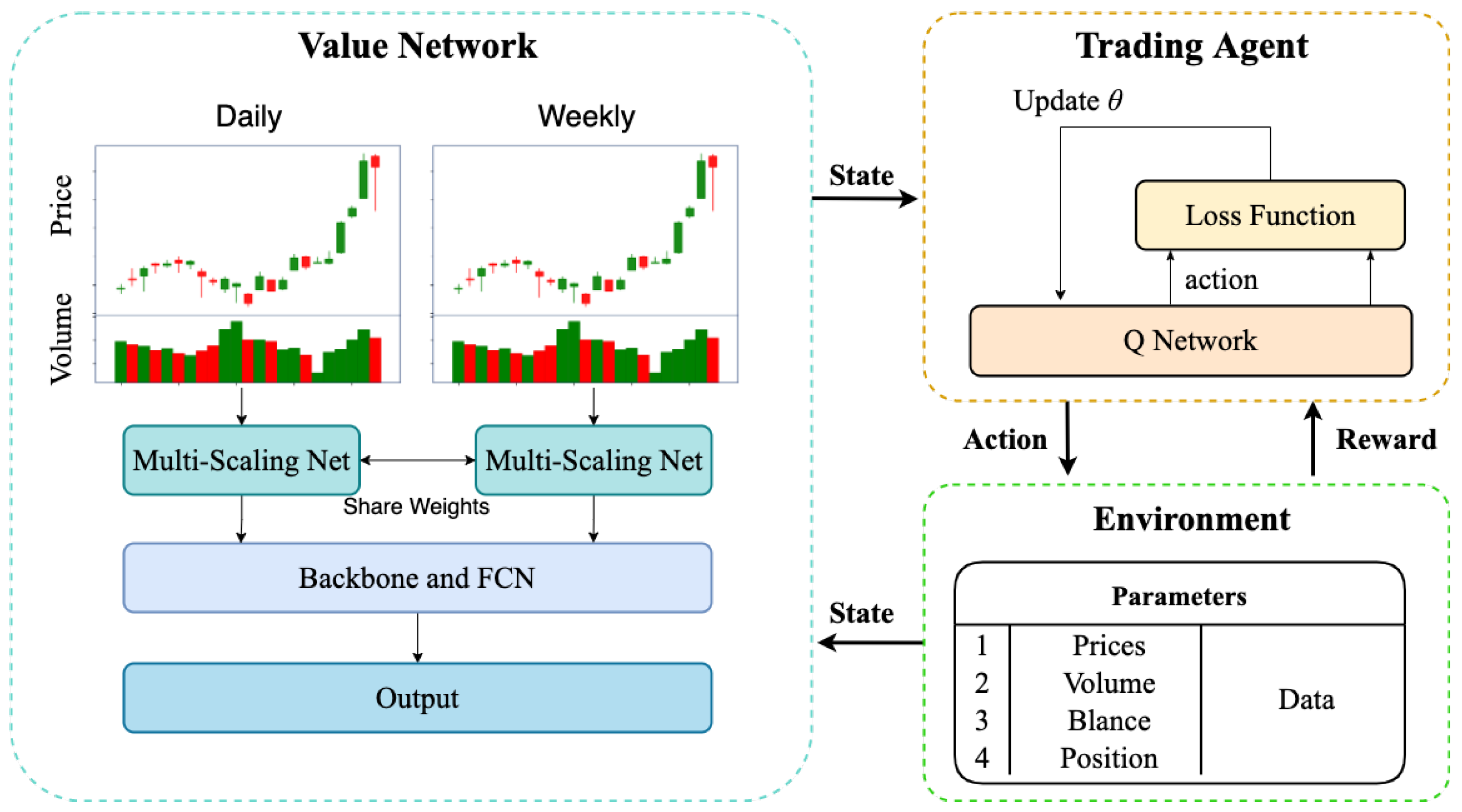
• Our research presents a new network structure, MS-CNN, for extracting multi-scaling features for studying financial markets. This network can automatically explore multi-scaling features of daily and weekly trading data through multi-scaling CNN, similar to the attention humans pay to information at different temporal and spatial scaling during stock trading. Additionally, we employ a backbone CNN to extract stock features and introduce an average pooling layer to prevent overfitting and enhance the network’s robustness. Our findings demonstrate that a multi-scaling CNN can detect more reliable information in this task.
• By taking advantage of the multi-scaling CNN, we propose the MS-CNN-SARSA model using an on-policy reinforcement learning algorithm, namely SARSA, which tends to avoid dangerous strategies in the presence of a large number of negative rewards when close to the optimal path. In this way, the agent is able to generate dynamic trading strategies by learning multi-scaling information on different time scaling on the stock market.
• Our experimental results on four real datasets demonstrate the significant performance of the proposed model. By extracting multi-scaling features, the agent can act over longer time scaling. To be more specific, the agent identifies a weekly low for a stock and buys at that point without being swayed by the daily fluctuations of the stock during successive declines. In addition, we performed several experiments of comparison and ablation to validate the excellent network structure. This includes comparing the performance of MS-CNN-SARSA using modules of different sizes and network structures with different activation functions.

The structure of this paper is outlined as follows. In Section 2, we discuss previous research on the topic. Section 3 provides a general formalization of the stock trading problem. Section 4 explains our proposed model in detail. The experimental results are presented and analyzed in Section 5. Finally, Section 6 summarizes our findings and outlines potential future research areas.

2. Literature Review

In this section, two bodies of literature are reviewed: research on reinforcement learning in finance and time series-based multi-scaling learning.

2.1. Reinforcement Learning in a Trading System

As artificial intelligence advances rapidly, an increasing number of researchers are focusing on automated financial trading systems to substitute human operators’ expertise, skills, and intuition in making investment decisions in financial markets. Among the various approaches, reinforcement learning has been utilized in single-asset trading systems, starting with Moody’s initial application of recurrent reinforcement learning to single stocks in 1999 [2]. Previous methods can be divided into two categories: value-based reinforcement learning [3,4,5] and policy-based reinforcement learning [2,6,7,8,9]. Value-based methods use the state value to indirectly approximate the optimal policy. For example, Corazza et al. applied Q-learning and SARSA to a simulated trading environment and evaluated their performance based on various metrics, including return on investment and the Sharpe ratio [4]. Policy-based methods directly approximate the optimal policy using the objective function. Recently, researchers have improved these techniques by combining reinforcement learning methods with deep learning. These methods can be divided into policy-based deep reinforcement learning [10,11,12,13,14] and value-based deep reinforcement learning [15,16,17,18,19,20,21,22,23,24]. For example, Corazza et al. compared the results obtained considering different policy-based (SARSA) and off-policy-based (Q-Learning, Greedy-GQ) reinforcement learning algorithms applied to daily transactions in the Italian stock market [19]. Cheng et al. combined long short-term memory and the deep Q-Network (DQN) to determine trading signals and the size of trading positions using price data from the Taiwan stock market, including daily opening and closing prices, high and low prices, and trading volume [23]. Recently, some researchers have combined various reinforcement learning techniques to address the more general problem of algorithmic trading. For example, Zhang et al. employed the DQN, policy gradient, and advantage actor critic to develop strategies for trading future contracts and modify transaction positions according to market fluctuations [25]. Jiang et al. combined long- and short-term risk (LSTR) control with the twin delayed deep deterministic policy gradient algorithm to build a portfolio model with risk management capabilities using Chinese stock data from the Shanghai Stock Exchange [26]. Li et al. used a long short-term memory and convolutional neural network combination to extract features from candlestick chart and raw trading data and applied Dueling DQN and Double DQN methods to generate the best strategy [27]. Wang et al. proposed a novel stock trading strategy consisting of two steps: turning point classification using LightGBM and reinforcement learning using DQN and related models. The strategy aimed to help investors make better decisions by effectively controlling risks and obtaining higher returns. Transaction trigger conditions were set to combine the two parts. In experiments, the proposed strategy outperformed long-term holding, reinforcement learning alone, and the actor-critic strategy in terms of returns [28]. Furthermore, some researchers have started expanding the usage of single-agent reinforcement learning to multi-agent reinforcement learning. Carta et al. proposed a multi-layer and multi-ensemble stock trader that pre-processes data with deep neural networks and used a reward-based classifier as a meta-learner to generate stock signals. The approach used several trading agents to make a final decision [29]. Shavandi et al. proposed a multi-agent deep reinforcement learning framework for algorithmic trading that was hierarchical in structure and robust to noise in financial time series. Each agent in a specific time frame was trained using the DQN algorithm [30].

2.2. Time Series-Based Multi-Scaling Learning

Multi-scaling learning is a novel approach in the realm of machine learning, where models gather and process data at multiple scaling [31]. Deep convolutional neural network models, such as AlexNet [32], oxford visual geometry group [33], faster-regions with CNN features [34], residual network [35], and you only live once [36,37,38,39], were often used as visual feature extractors for various tasks, such as object detection, object segmentation, and image classification. In financial series data, Kirisci used a CNN-based forecasting model for financial time series that preserved the time sequence effect and avoided information loss. The model was composed of three convolutional layers and five fully connected layers with rectified linear unit and exponential linear unit activation functions [40]. Although these methods are commonly used, they mostly consider single-scaling input and do not focus on multi-scaling processing. By extracting feature maps with various scaling, the convolutional neural networks can enhance their representation ability. U-Net was a symmetric encoder–decoder structure proposed by Ronneberger et al. that incorporated high-level and low-level features to extract more abundant multi-scaling features [41]. The inception family of convolutional neural networks was proposed by Szegedy et al., which improved performance by learning each block of multi-scaling features using various scaling of convolutional computations [42,43,44]. A novel multi-scaling convolutional network was introduced by Yang et al. that utilized the attention mechanism in the Res2-block structure to improve image feature extraction [45].

However, numerous research efforts have focused on extracting multi-scaling information from financial series [46]. Some approaches used different network capabilities for different scaling to generate more powerful multi-scaling features by fusing at multiple levels of the network model. The effectiveness of multi-scaling neural network architectures for time series prediction of nonlinear dynamic systems was investigated by Geva et al. The architectures decompose the time series into different scaling using wavelet transforms and extract features from each scaling using multiple neural networks [47]. Cui et al. introduced a multi-scaling convolutional neural network to extract features at various scaling and frequencies automatically, which resulted in more effective feature representation [48]. Liu et al. proposed a method for extracting multiple data features based on single and multiple time steps that combines the short- and long-time features to improve the prediction accuracy. These methods brought significant improvements in using multi-scaling information in comparison to single-scaling techniques [49]. Teng et al. introduced multi-scale local cues and a hierarchical attention-based LSTM model to catch potential price tendency patterns to maximize stock investment returns [50].

Based on the literature review, previous studies on reinforcement learning in the financial domain have mainly focused on single-scaling data without using sliding windows to analyze stock data at different scaling. This means that other types of data, such as weekly data, have been overlooked. However, combining reinforcement learning with time series analysis and multi-scaling feature fusion can help agents consider information at higher scaling and provide better trading strategies according to the present market conditions. Additionally, no prior research has combined multi-scaling learning and reinforcement learning in finance. This study proposes the MS-CNN-SARSA model, which employs the SARSA framework and a multi-scaling deep convolutional neural network to extract short-term and long-term trends from stock data at two time units. This approach aims to develop more effective transaction strategies.

3. The Formulation of Problem

The problem of algorithmic trading as a sequential decision process is framed in this section as a Markov decision process in reinforcement learning.

State Space: The present state of a stock could be described by a set of features that typically included information such as historical prices and transaction volumes. Taghian et al. [51] compared the effect of window sizes of 3–75 on the extraction of appropriate patterns for each asset from the input candlesticks. According to the experiments, it had been observed that the most appropriate pattern extraction could be achieved with a window length of 10 to 20 for each asset using a sequence of candlesticks. In our study, we used the opening, highest, lowest, and closing prices and transaction volume of the past m = 20 days and weeks for the current state with time step t. Figure 1 shows two continuous states.

Action Space: The available actions for agents were defined in a discrete action space where the policy involved opening, holding, or closing a position in a single asset. This policy assumes the buying and selling of a stock, and the position information is represented by an integer scalar ${\mathrm{POS}}_t$, which indicates the value of the current position at time t.

$$\begin{array}{c}\hfill {\mathrm{POS}}_t=\left\{\begin{array}{cc}1,\hfill & \hfill \mathrm{opening}\mathrm{a}\mathrm{long}\mathrm{position},\\ 0,\hfill & \hfill \mathrm{no}\mathrm{position},\\ -1,\hfill & \hfill \mathrm{opening}\mathrm{a}\mathrm{short}\mathrm{position}.\end{array}\right.\end{array}$$

(1)

In this paper, we assumed that the action taken by the agent would not affect the financial market. ${\mathrm{POS}}_0=0$ implied that the agent had no position from the start. ${\mathrm{POS}}_t=1$ represented that the agent held the long position. ${\mathrm{POS}}_t=-1$ represented that the agent held the short position. Moreover, we obtained the final action $a_t\in A=\{-1,0,1\}=\{\mathrm{Sell},\mathrm{Hold},\mathrm{Buy}\}$.

Reward: Every action that the agent takes has a corresponding reward, and the agent’s goal is to maximize cumulative returns. In this paper, we designed a reward function based on risk-adjusted returns, which could be considered by combining risk and return metrics, such as the Sharpe ratio [52]. The Sharpe ratio is a widely used measurement in finance that evaluates the risk-adjusted performance of an investment strategy by considering the return and risk involved. In addition, the Sharpe ratio was also used as a reward function in [4,19,27]. Therefore, the reward function chosen was the short-term Sharpe ratio, which took into account future information for n days and emphasized information about the agent’s position. It should be noted that our reward function did not take into account the transaction costs, which could lead to high turnover rates and thus affect the profitability of the trading strategy. The sum of the Sharpe ratios for a given period represented the cumulative risk-adjusted returns achieved by the trading system for that particular period. Since rewards were random variables, summing these Sharpe ratios helped reduce the effects of randomness and provided an approximation of the expected value of the cumulative rewards. The reward function was represented by this choice.

$$SS{R}_t={\mathrm{POS}}_t\ast S{R}_t,$$

(2)

where

$$\begin{array}{cc}\hfill S{R}_t& =\frac{\mathrm{mean}\left(R_t^n\right)}{\mathrm{std}\left(R_t^n\right)},\hfill \\ \hfill R_t^n& =[\frac{p_{t+1}-p_t}{p_t},\frac{p_{t+2}-p_t}{p_t},\cdots ,\frac{p_{t+n}-p_t}{p_t}].\hfill \end{array}$$

where $p_t$ referred to the closing price during t.

4. Methodology

The specific details of the introduced trading system with multi-scaling enhancements are discussed in this section. Firstly, the framework of MS-CNN-SARSA is described. Although SARSA is useful in solving reinforcement learning problems, it has limitations in its feature extraction capability. We designed the MS-CNN model to solve the mentioned problem. Secondly, weekly prices and trading volume information as multi-scaling features are introduced into the DCNN model. Finally, the multi-scaling CNN (MS-CNN) model is presented.

4.1. System Overview

This section briefly introduces our multi-scaling reinforcement trading system, including the SARSA and the multi-scaling convolutional network. Compared with the proposed trading system in the previous study, our proposed system combined data from multi-scaling of stock data to construct a multi-scaling reinforcement learning framework. Our proposed trading system was composed of two parts. In the first part, data at different multi-scaling, including daily and weekly trading data, were extracted and processed by independent neural networks. In the second part, the reinforcement learning algorithm was performed. The agent first perceived the state, then performed the actions determined by its policy, and received rewards based on its performance. Finally, interacting with the environment in a reinforcement learning framework generated the best trading strategy. A great trading strategy is not focused on maximizing profits from individual trades but on achieving sustainable profits over time. A framework diagram of a multi-scaling CNN reinforcement learning trading system can be seen in Figure 2.

As illustrated in Figure 2, during each step t, the agent executed a series of trades with corresponding rewards $\{r_1,\cdots ,r_t,\cdots ,r_T\}$. By considering the observed transactions, the expected value of $U_t\left(s_t\right)$ can be estimated as follows:

$$\begin{array}{cc}\hfill Q_{\pi }(s_t,a_t)& =\mathbb{E}[U_t\mid S_t=s_t,A_t=a_t]\hfill \\ \hfill & =\mathbb{E}[r_t+\gamma U_{t+1}\mid S_t=s_t,A_t=a_t]\hfill \\ \hfill & =\mathbb{E}[r_t+\gamma Q_{\pi }(S_{t+1},A_{t+1})\mid S_t=s_t,A_t=a_t].\hfill \end{array}$$

(3)

where $U_t$ refers to the discounted return, which indicates the agent’s expected return, and is defined as follows:

$$U_t=r_t+\gamma r_{t+1}+\cdots +{\gamma }^{T-t}{r}_T,$$

(4)

where $\gamma$ refers to the discount factor, $\gamma \in [0,1]$.

$Q_{\pi }(s_t,a_t)$ represents the expected benefit of taking an action $a_t$ at the present state $s_t$. For updating the action value function in the present state, we applied the following state-action value function as an estimate. Herein, we employed the on-policy value-based approach, SARSA (state, action, reward, state, action), to attain the best state-action value function [53]. Consequently, the equation is updated as:

$$Q_{\pi }(s_t,a_t)\leftarrow Q_{\pi }(s_t,a_t)-\alpha [r_t+\gamma Q_{\pi }(s_{t+1},a_{t+1})-Q_{\pi }(s_t,a_t)].$$

(5)

The temporal-difference value was calculated using the present state’s action value and the next state’s action value. This implies that the next action generated by the policy must be known to execute the update step. Given the abundance of market states, we transformed the task of updating the Q-value table into a function approximation problem.

4.2. The Structure of Q-Network Based on Multi-Scaling CNN

This study put forward a framework, named MS-CNN, which is illustrated in Figure 3. The MS-CNN model was trained on both daily and weekly stock data.

Inspired by computer vision networks, our network was composed of three parts. Each part had a different function, eventually linking each part together to achieve stock price prediction in multiple time perspectives.

Multi-Scaling Net: By mimicking human stock trading behavior, our network considered daily trading data and weekly stock charts to make decisions on a global scaling. Considering that, in the image task, the image was composed of three-color channels, R, G, and B, the prediction result was determined by these three channels simultaneously. We decided to use a network that combined daily data sessions and weekly data into a single feature map. Furthermore, considering that human behavior combines five stock indicators to think about, we used different scaling of convolution in our design to mimic human multi-scaling considerations.

The multi-scaling network was composed of three feature extraction modules at different scaling. The first module was a single-scaling feature extractor, which extracted time-domain features with five parameters using a one-dimensional convolution technique to stack into five-dimensional features. The second module was the medium-scaling feature extractors, which viewed the data for the single channel two-dimensional image and applied two-dimensional convolution using $3\times 3$ convolution kernel size. The third module was the global-scaling feature extractors, which considered single-channel image data and performed global feature extraction using a convolution kernel size of $5\times 5$. Then, these three modules’ outputs were concatenated into an eight-channel, two-dimensional feature layer to be considered the multi-scaling net output. It is worth mentioning that the daily and weekly nets shared the same weight parameters. Specifically, we shared the same multi-scaling network for both weekly and daily data to ensure that the same parameters were used in the weekly and daily stock data modules; that is, they use the same convolution kernel and pooling window size when performing convolution and pooling operations. The purpose of our model is to make judgments on both the weekly and daily scaling at the same time, so the two should not be independent. At the same time, the weekly and daily charts should be similar in terms of the characteristics of the stock. Sharing weights could increase the number of samples in the multi-scaling net and increase the generalization of the network. Figure 3 shows the overall architecture of the multi-scaling net.

Backbone: We used the backbone convolutional neural network to extract stock features and added an average pooling layer to the backbone network to prevent overfitting and increase the robustness of the network. The attention module has also been widely shown to improve model performance in image tasks, so we added the attention module to the network backbone.

Fully Connected Net: As the final output part of our network model, we obtained the final output representing the three trading action (buy, hold, and sell) scores using two fully connected layers.

The objective of this neural network was to calculate an approximation of the action value function $Q(s,a;w)$ for the market environment, where w represented the network weights and biases. While the state space was continuous or large, it was beneficial to use function approximations. In order to acquire the present best state-action value, this network followed the $ϵ-$greedy method, where it selected one action $a_t$ according to the current state $s_t$, and subsequently observed the next state $s^{\prime }$ and the associated reward $r_t$. The resulting current state-action value was $Q(s_t,a_t)$:

$$Q^{*}(s_t,a_t)=\mathbb{E}[r_t+\gamma Q(S_{t+1},A_{t+1})\mid S_t=s_t,A_t=a_t],$$

(6)

where $a_{t+1}$ represents the action that would be chosen at the next time step according to the $ϵ-$greedy.

4.3. MS-CNN-SARSA Algorithm

State, action, reward, state, action (SARSA), as part of the reinforcement learning algorithm, was an on-policy method. The SARSA algorithm was a small variant of the popular Q-Learning algorithm. Here, the SARSA algorithm was used to develop the best trading strategy through interaction with the environment. During the trading procedure, the agent would receive positive rewards if it chose profitable trading actions and negative rewards if it made losses. Such rewards acted as incentives for the agent to make appropriate choices during future trading actions.

Given the state $s_t$, the SARSA network needed to have three outputs that represented three distinct state-action values. The policy network, MS-CNN, processed the present state $s_t$ and produced a three-dimensional vector Q as the current state-action value. Then, the $ϵ-$greedy algorithm was used to select the current action a. Subsequently, it was observed for the reward $r_t$ and the next state $s_{t+1}$. To estimate the present $Q(s_t,a_t)$, the next state action value $Q(s_{t+1},a_{t+1})$ was obtained according to Equation (5). The training procedure for MS-CNN-SARSA is described in detail in Algorithm 1.

Algorithm 1 MS-CNN-SARSA Algorithm

Input: opening, high, low, closing prices, and transaction volume; 1: Initialize data stack D with a size of N; 2: Initialize the policy network (MS-CNN) with random weights w; 3: for episode = 1 to N do 4:     Initialize sequence $s_1=\left\{x_1\right\}$ and pre-process state ${\varphi }_1=\varphi \left(s_1\right)$; 5:     Select $a_1$ with $ϵ-$greedy method; 6:     for t=1 to T do 7:         Execute the action $a_t$ in the environment and get reward $r_t$ and observe next state $s_{t+1}$, ${\varphi }_{t+1}=\varphi \left(s_{t+1}\right)$; 8:         Store the transition $({\varphi }_t,a_t,r_t,{\varphi }_{t+1},a_{t+1})$ into stack D; 9:         Sample data from stack D; 10:         Select $a_{t+1}$ with $ϵ-$greedy method; 11:         Set: $$\begin{array}{c}\hfill y_i=\left\{\begin{array}{cc}{r}_i,\hfill & \hfill \mathrm{if}\mathrm{the}\mathrm{end}\mathrm{of}\mathrm{step}i+1,\\ r_i+\gamma Q({\varphi }_{t+1},a_{t+1};w)),\hfill & \hfill \mathrm{otherwise}.\end{array}\right.\end{array}$$ 12:         Training networks by loss functions $L\left(w\right)=\mathbb{E}\left[{(y_i-Q({\varphi }_i,a_i;w))}^2\right]$; 13:         $s_t\leftarrow s_{t+1};a_t\leftarrow a_{t+1}$; 14:     end for 15: end for

5. Experiments and Results

5.1. Dataset

The evaluation was performed on four real-world stock datasets, Dow Jones (DJIA), NASDAQ, General Electric (GE), and AAPLE (AAPL), collected from Yahoo Finance. The historical price data ranged from 1 January 2007 to 31 December 2017. Our experiment divided these data into two groups: the training set was composed of data from 1 January 2007 to 31 December 2017, while the test set contained data from 1 January 2018 to 31 December 2020.

Figure 4 presents the close price variations in DJIA, NASDAQ, AAPL, and GE. The orange line represents the training period, and the blue line represents the testing period. It could be observed that NASDAQ and AAPL kept rising while GE fell and DJIA exhibited irregular fluctuations.

5.2. Evaluation Indicators

In order to conduct a thorough and unbiased evaluation of a trading strategy’s performance, we chose three evaluation metrics, as outlined below.

• Profit: The profit of trading activities is a measure of the capital that has been gained or lost. To determine the profit at each time step t, we utilized Equation (7), which involved calculating the profit using the present amount $C_t$ and the initial amount $C_0$.

  $${\mathrm{Profit}}_t=C_t-C_0.$$

  (7)
• Sharpe ratio (SR): This ratio shows the average return earned per unit of total risk over the risk-free rate, which is computed in Equation (8), where $r_f$ refers to the risk-free asset return and $E\left\{r_p\right\}$ refers to the expected value of the portfolio value. We assumed $r_f=0$ in this study.

  $$\mathrm{SR}=\frac{\mathbb{E}\left\{r_p\right\}-r_f}{{\sigma }_p}.$$

  (8)
• Annualized return (AR): AR represents an investment’s average percentage of profits and losses generated through trading activity over a one-year period.

  $$\mathrm{AR}=({(1+\mathrm{CR})}^{\frac{365}{\mathrm{Days}\mathrm{Held}}}-1)\ast 100.$$

  (9)

  where CR is calculated by ${\sum }_{t=1}^T\frac{C_t-C_{t-1}}{C_{t-1}}$.

5.3. Baseline Methods

In order to assess the performance of our proposed method, we compared the proposed MS-CNN-SARSA algorithm with value-based reinforcement learning methods, such as DQN-Pattern and DQN-Vanilla, and some traditional trading strategies, such as buy and hold and sell and hold.

• Buy and hold: This involves the investor choosing an investment asset with a long position in the initial investment phase. Once the asset is purchased, it is held until the end of the period, regardless of any changes in its price.
• Sell and hold: This involves the investor choosing an investment asset with a short position in the initial investment phase. Once the asset is purchased, it is held until the end of the period, regardless of any changes in its price.
• DQN-Pattern: This learns suitable trading patterns according to candlestick patterns for a specific stock. More details can be seen in [24].
• DQN-Vanilla: This involves using raw candlestick data to train a fitted learning algorithm to create trading rules. More details can be seen in [24].

5.4. Experimental Setup

We evaluated the proposed approach against four baseline approaches, namely the DQN-Pattern, DQN-Vanilla, buy and hold, and sell and hold strategies. The initial capital was fixed at USD 500,000. In the U.S. stock market, the transaction fees are typically calculated as a fixed amount per trade or a percentage of the trade amount. The exact amount of transaction fees could vary depending on factors such as the broker, the exchange, and the size of the transaction. In general, trading fees are relatively low in the U.S. stock market, especially for the average retail investor. Competition among broker-dealers has also led to declining trading fees. In this paper, we used 0.01% as the percentage of transaction costs that reflected true transaction costs to a certain extent. However, it was important to note that transaction costs in real-world markets could vary and include factors such as spreads, fees, and commissions. Herein, we chose to use a relatively small cost term as a simplification and focus primarily on evaluating the performance of our proposed reinforcement learning trading system. The discounter factor was set at 0.9, and the exploration probability gradually decreased from 0.9 to 0.05. Window lengths were set to 20 for daily and weekly. Notably, we removed the marginal data from the dataset to avoid the extreme problem of the Sharpe ratio since its reward requires data from the next 5 days.

In order to keep the data inputs within a rational range, we utilized data normalization techniques. The Adam algorithm, with a fixed learning rate of 0.001, was used to optimize all models. All models from the Pytorch library were implemented by terminating the training after 100 iterations. The DQN-Pattern and DQN-Vanilla approaches were implemented using the code provided by [24].

5.5. Experimental Results

In this section, we structure our work into three main parts. Firstly, we enhance the comparison with existing methods by conducting a comprehensive evaluation of our proposed approach against well-established and widely recognized trading strategies. We incorporate additional performance metrics, such as profit, Sharpe ratio, and annualized return, to provide a more comprehensive assessment of the effectiveness of our method. Secondly, we conducted experiments to compare the performance of our method using features extracted solely from daily financial data with features extracted from both daily and weekly financial data. This comparative analysis allows us to demonstrate the superiority of our proposed method over single-scaling methods. Lastly, we conducted experiments using different activation functions and compared their performance. Through this analysis, we provide empirical evidence supporting the selection of the Tanh activation function in our method.

Several experiments were conducted in the U.S. stock market to demonstrate the efficacy of the proposed MS-CNN-SARSA algorithm. First, we conducted a performance comparison of our proposed method with a baseline on stock indices, such as DJIA, NASDAQ, AAPL, and GE, separately. Second, we selected individual stocks in each of the two categories of bullish and bearish markets, such as AAPL and GE. The performance of the MS-CNN-SARSA algorithm and several baseline algorithms are presented in

Table 1. The performance of various trading approaches on four datasets.

Datasets	Indicators	Buy and Hold	Sell and Hold	DQN-Pattern	DQN-Vanilla	SARSA
DJIA	Profit	53,608	−53,608	59,233	83,737	299,740
	SR	0.304	−0.079	0.325	0.414	0.996
	AR	11.34	−2.88	12.16	13.97	32.66
NASDAQ	Profit	239,668	−239,668	234,454	283,431	394,018
	SR	0.803	−0.744	0.787	1.000	1.245
	AR	28.92	−39.82	28.49	31.03	38.60
AAPL	Profit	679,847	−679,847	640,594	766,268	1,341,994
	SR	1.271	−0.234	1.230	1.563	2.061
	AR	57.80	−100.00	55.95	59.22	78.41
GE	Profit	−273,017	273,017	31,425	794,302	950,557
	SR	−0.425	0.918	0.673	1.831	1.301
	AR	−35.55	30.71	4.09	58.84	72.26

, and the change in total capital with different assets is depicted in Figure 5, Figure 6, Figure 7 and Figure 8. Based on these findings, it could be inferred that the cumulative return ratio of the MS-CNN-SARSA algorithm outperformed the other baseline algorithms for most stocks. Additionally, the annualized return of the MS-CNN-SARSA algorithm was significantly higher than that of the other baseline algorithms. The Sharpe ratio also increased significantly, which meant that investors could have a higher return for each unit of risk. The results for various assets demonstrated the efficacy of the MS-CNN-SARSA algorithm. Overall, the findings in Table 1 suggest that the proposed MS-CNN-SARSA algorithm could enhance the performance of agents and generate more consistent benefits.

In addition, Figure 5, Figure 6, Figure 7 and Figure 8 show the performance of several models, where the initial cash was set at USD 500,000 and the purple lines represent the proposed MS-CNN-SARSA algorithm. Among all of the assets, the purple line of the proposed algorithm consistently outperformed the other curves. The purple curves tended to maintain an upward trend even when there were significant price fluctuations, indicating the MS-CNN-SARSA algorithm’s robustness and superior performance compared to other baseline methods, particularly in a bearish market. Additionally, the results of the GE stock showed that the proposed method could generate higher profits than the other benchmarks during price declines. These findings further support the effectiveness of the MS-CNN-SARSA algorithm in achieving steady profits, regardless of market fluctuations.

Figure 9, Figure 10, Figure 11 and Figure 12 present the trading signals of the MS-CNN-SARSA algorithms. We found that agents could generate correct trading signals in positions where market trends changed. It could be seen that the MS-CNN-SARSA strategy could accurately detect the market trend and hedge the risk by changing the position direction at times when the market fluctuates drastically. For example, the agent learned that it was more profitable to open a short position than other actions and chose to hold a short position in GE stock. That was because the market was mostly bearish. As we observed, such as in the markets of DJIA, NASDAQ, and AAPL, the agent understood that it was more profitable to open a long position than other actions and chose to hold a long position. The reason for this was that the market was bullish most of the time.

The results indicate that making profits in a market that was experiencing a bullish trend was relatively simple, but it could be challenging to achieve consistent profits or avoid losses when the market was experiencing a bearish or consolidation trend. However, the results obtained from the experiments demonstrate that the proposed MS-CNN-SARSA algorithm could consistently generate profits, regardless of the market state.

Table 2. The comparison on different time scaling.

Dataset	Indicators	Single-Scaling	Multi-Scaling
DJIA	Profit	140,750	299,740
	SR	0.570	0.996
	AR	20.22	32.66
NASDAQ	Profit	337,034	394,018
	SR	1.073	1.245
	AR	35.3	38.60
AAPL	Profit	763,222	1,341,994
	SR	1.439	2.061
	AR	60.3	78.41
GE	Profit	518,108	950,557
	SR	0.931	1.301
	AR	54.85	72.26

presents the results of comparing the single-scaling and multi-scaling modules in the proposed MS-CNN-SARSA algorithm. The single-scaling module used only daily data and had the same structure as the multi-scaling module, except for the feature extraction method. The multi-scaling module, on the other hand, utilized daily and weekly data to extract features. The results clearly show that the multi-scaling modules outperform the single-scaling modules, with the GE dataset achieving a Sharpe ratio of $1.301$ and an annualized return of $72.26\%$. The main difference between the two modules was the feature extraction method, with the multi-scaling module using both daily and weekly data to capture both local and global features, while the single-scaling module only used daily data to focus on local features. The results highlighted the importance of incorporating multi-scaling information in the algorithm, demonstrating the effectiveness of the multi-scaling feature.

Table 3. The comparison of SARSA to various activation functions.

Dataset	Indicators	Tanh	ELU	ReLU	SiLU
DJIA	Profit	299,740	82,890	293,075	124,262
	SR	0.996	0.395	0.996	0.533
	AR	32.66	14.33	31.82	17.96
NASDAQ	Profit	394,018	371,022	330,909	952,494
	SR	1.245	1.121	1.075	2.246
	AR	38.60	37.68	34.75	64.12
AAPL	Profit	1,341,994	1,356,284	999,571	1,239,528
	SR	2.061	2.064	1.699	1.893
	AR	78.41	78.83	68.74	76.17
GE	Profit	950,557	240,908	156,689	15,065
	SR	1.301	0.626	0.498	0.262
	AR	72.26	36.41	33.63	16.93
Mean	Profit	746,577.25	512,776.00	445,061.00	582,837.25
	SR	1.401	1.052	1.067	1.234
	AR	55.48	41.81	42.24	43.08

displays the performance comparison of various activation functions, namely ELU, ReLU, SiLU, and Tanh, in the MS-CNN-SARSA algorithm. The other parameters were set as the corresponding settings in the MS-CNN-SARSA method. Based on the results of the different activation functions, it was observed that the Tanh activation function was better suited for the proposed model than the other activation functions. Tanh could take any real value as the input and produce output values in the range of $-1$ to 1. If the input was more positive, the output value was closer to 1, and if the input was more negative, the output value was closer to $-1$.

6. Conclusions and Future Work

Inspired by the multi-scaling feature fusion in vision tasks, we propose a novel trading system called the multi-scaling CNN SARSA (MS-CNN-SARSA). This trading system integrates SARSA, convolutional neural networks, and multi-scaling feature fusion to extract features from daily and weekly financial data to generate trading strategies. In this way, the agent not only makes decisions based on daily trading data but also takes the weekly stock charts into consideration to make decisions on a global scaling. Experimental results in the U.S. stock market show that the proposed MS-CNN-SARSA algorithm can achieve excess returns when the stock market has high volatility and change the direction of positions in time to capture market trends accurately. It can gain more profit and take less risk in both bearish and bullish markets. In particular, the comparison results of both single-scaling and multi-scaling modules show that the multi-scaling performance is better than the single-scaling one.

In this paper, we propose a new trading algorithm based on the deep reinforcement learning algorithm that is better than the other existing models. However, some other studies can still be extended in the future. Firstly, introducing more time scaling, such as hour and minute data. Secondly, it is important for the agent to identify the current market state by considering other market information, such as news and macroeconomics. However, the proposed MS-CNN-SARSA algorithm only considers raw trading data. Furthermore, while the algorithm shows good performance in trading a single stock, more research is needed to explore its application in portfolio management. Finally, the proposed new trading algorithm should consider the legal costs and risks of data protection in the U.S. and other legal regimes. For instance, informed consent by the users of stock exchanges is needed for the use of personal data. This may undermine the efficiency and accuracy of the operation of the new trading algorithm. The new method should also be able to ensure data security during the processing of the algorithm. Further studies may take these risks and costs into consideration.

References

1. Poterba, J.M.; Summers, L.H. Mean Reversion in Stock Prices: Evidence and Implications; Social Science Electronic Publishing: London, UK, 1988. [Google Scholar]
2. Moody, J.E.; Saffell, M.J. Reinforcement learning for trading. In Proceedings of the NIPS’98: 11th International Conference on Neural Information Processing Systems, Denver, CO, USA, 30 November–5 December 1998; Volume 17, pp. 917–923. [Google Scholar]
3. Neuneier, R. Enhancing Q-learning for optimal asset allocation. In Proceedings of the NIPS’98: 11th International Conference on Neural Information Processing Systems, Denver, CO, USA, 30 November–5 December 1998; pp. 936–942. [Google Scholar]
4. Corazza, M.; Sangalli, A. Q-Learning and SARSA: A Comparison between Two Intelligent Stochastic Control Approaches for Financial Trading. SSRN Electron. J. 2015. [Google Scholar] [CrossRef]
5. Yan, C.; Mabu, S.; Hirasawa, K. Genetic network programming with sarsa learning and its application to creating stock trading rules. In Proceedings of the 2007 IEEE Congress on Evolutionary Computation, Singapore, 25–28 September 2007; pp. 220–227. [Google Scholar]
6. Moody, J.; Saffell, M. Learning to trade via direct reinforcement. IEEE Trans. Neural Netw. 2001, 12, 875–889. [Google Scholar] [CrossRef] [PubMed]
7. Gold, C. FX trading via recurrent reinforcement learning. In Proceedings of the 2003 IEEE International Conference on Computational Intelligence for Financial Engineering, Hong Kong, China, 20–23 March 2003; pp. 363–370. [Google Scholar]
8. Zhang, J.; Maringer, D. Indicator selection for daily equity trading with recurrent reinforcement learning. In Proceedings of the 15th Annual Conference Companion on Genetic and Evolutionary Computation, Amsterdam, The Netherlands, 6–10 July 2013; pp. 1757–1758. [Google Scholar]
9. Zhang, J.; Maringer, D. Using a genetic algorithm to improve recurrent reinforcement learning for equity trading. Comput. Econ. 2016, 47, 551–567. [Google Scholar] [CrossRef]
10. Yue, D.; Feng, B.; Kong, Y.; Ren, Z.; Dai, Q. Deep Direct Reinforcement Learning for Financial Signal Representation and Trading. IEEE Trans. Neural Netw. Learn. Syst. 2016, 28, 653–664. [Google Scholar]
11. Liu, F.; Li, Y.; Li, B.; Li, J.; Xie, H. Bitcoin transaction strategy construction based on deep reinforcement learning. Appl. Soft Comput. 2021, 113, 107952. [Google Scholar] [CrossRef]
12. Mahayana, D.; Shan, E.; Fadhl’Abbas, M. Deep Reinforcement Learning to Automate Cryptocurrency Trading. In Proceedings of the 2022 12th International Conference on System Engineering and Technology (ICSET), Bandung, Indonesia, 3–4 October 2022; pp. 36–41. [Google Scholar]
13. Tsai, Y.-C.; Szu, F.-M.; Chen, J.-H.; Chen, S.Y.-C. Financial Vision-Based Reinforcement Learning Trading Strategy. Analytics 2022, 1, 35–53. [Google Scholar] [CrossRef]
14. Xiao, X. Quantitative Investment Decision Model Based on PPO Algorithm. Highlights Sci. Eng. Technol. 2023, 34, 16–24. [Google Scholar] [CrossRef]
15. Si, W.; Li, J.; Ding, P.; Rao, R. A multi-objective deep reinforcement learning approach for stock index future’s intraday trading. In Proceedings of the 2017 10th International Symposium on Computational Intelligence and Design (ISCID), Hangzhou, China, 9–10 December 2017; Volume 2, pp. 431–436. [Google Scholar]
16. Huang, C.Y. Financial trading as a game: A deep reinforcement learning approach. arXiv 2018, arXiv:1807.02787. [Google Scholar]
17. Chen, L.; Gao, Q. Application of Deep Reinforcement Learning on Automated Stock Trading. In Proceedings of the 2019 IEEE 10th International Conference on Software Engineering and Service Science (ICSESS), Beijing, China, 18–20 October 2019; pp. 29–33. [Google Scholar]
18. Chakraborty, S. Capturing financial markets to apply deep reinforcement learning. arXiv 2019, arXiv:1907.04373. [Google Scholar]
19. Corazza, M.; Fasano, G.; Gusso, R.; Pesenti, R. A Comparison among Reinforcement Learning Algorithms in Financial Trading Systems; Research Paper Series No. 33; University Ca’Foscari of Venice, Department of Economics: Venice, Italy, 2019. [Google Scholar]
20. Li, Y.; Ni, P.; Chang, V. Application of deep reinforcement learning in stock trading strategies and stock forecasting. Computing 2020, 102, 1305–1322. [Google Scholar] [CrossRef]
21. Wu, X.; Chen, H.; Wang, J.; Troiano, L.; Fujita, H. Adaptive Stock Trading Strategies with Deep Reinforcement Learning Methods. Inf. Sci. 2020, 538, 142–158. [Google Scholar] [CrossRef]
22. Shi, Y.; Li, W.; Zhu, L.; Guo, K.; Cambria, E. Stock trading rule discovery with double deep Q-network. Appl. Soft Comput. 2021, 107, 107320. [Google Scholar] [CrossRef]
23. Cheng, L.C.; Huang, Y.H.; Hsieh, M.H.; Wu, M.E. A novel trading strategy framework based on reinforcement deep learning for financial market predictions. Mathematics 2021, 9, 3094. [Google Scholar] [CrossRef]
24. Taghian, M.; Asadi, A.; Safabakhsh, R. Learning financial asset-specific trading rules via deep reinforcement learning. Expert Syst. Appl. 2022, 195, 116523. [Google Scholar] [CrossRef]
25. Zhang, Z.; Zohren, S.; Roberts, S. Deep reinforcement learning for trading. J. Financ. Data Sci. 2020, 2, 25–40. [Google Scholar] [CrossRef]
26. Jiang, C.; Wang, J. A Portfolio Model with Risk Control Policy Based on Deep Reinforcement Learning. Mathematics 2022, 11, 19. [Google Scholar] [CrossRef]
27. Li, Y.; Liu, P.; Wang, Z. Stock Trading Strategies Based on Deep Reinforcement Learning. Sci. Program. 2022, 2022, 4698656. [Google Scholar] [CrossRef]
28. Wang, J.; Jing, F.; He, M. Stock Trading Strategy of Reinforcement Learning Driven by Turning Point Classification. Neural Process. Lett. 2022, 1–20. [Google Scholar] [CrossRef]
29. Carta, S. A multi-layer and multi-ensemble stock trader using deep learning and deep reinforcement learning. Appl. Intell. Int. J. Artif. Intell. Neural Netw. Complex Probl. Solving Technol. 2021, 51, 889–905. [Google Scholar] [CrossRef]
30. Shavandi, A.; Khedmati, M. A multi-agent deep reinforcement learning framework for algorithmic trading in financial markets. Expert Syst. Appl. 2022, 208, 118124. [Google Scholar] [CrossRef]
31. Wang, Y.; Wun Cheung, S.; Chung, E.T.; Efendiev, Y.; Wang, M. Deep Multiscale Model Learning. J. Comput. Phys. 2018, 406, 109071. [Google Scholar] [CrossRef]
32. Krizhevsky, A.; Sutskever, I.; Hinton, G.E. ImageNet Classification with Deep Convolutional Neural Networks. In Proceedings of the Annual Conference on Neural Information Processing Systems, Lake Tahoe, NV, USA, 3–8 December 2012. [Google Scholar]
33. Simonyan, K.; Zisserman, A. Very Deep Convolutional Networks for Large-Scale Image Recognition. arXiv 2014, arXiv:1409.1556. [Google Scholar]
34. Ren, S.; He, K.; Girshick, R.B.; Sun, J. Faster R-CNN: Towards Real-Time Object Detection with Region Proposal Networks. In Proceedings of the Annual Conference on Neural Information Processing Systems, Montreal, QC, Canada, 7–12 December 2015; Volume 28. [Google Scholar]
35. He, K.; Zhang, X.; Ren, S.; Sun, J. Deep Residual Learning for Image Recognition. In Proceedings of the 2016 IEEE Conference on Computer Vision and Pattern Recognition (CVPR), Las Vegas, NV, USA, 27–30 June 2016; pp. 770–778. [Google Scholar]
36. Redmon, J.; Divvala, S.K.; Girshick, R.B.; Farhadi, A. You Only Look Once: Unified, Real-Time Object Detection. In Proceedings of the 2016 IEEE Conference on Computer Vision and Pattern Recognition (CVPR), Las Vegas, NV, USA, 27–30 June 2016; pp. 779–788. [Google Scholar]
37. Redmon, S.; Farhadi, A. YOLO9000: Better, Faster, Stronger. In Proceedings of the 2017 IEEE Conference on Computer Vision and Pattern Recognition (CVPR), Honolulu, HI, USA, 21–26 July 2017; pp. 6517–6525. [Google Scholar]
38. Redmon, S.; Farhadi, A. YOLOv3: An Incremental Improvement. arXiv 2018, arXiv:1804.02767. [Google Scholar]
39. Bochkovskiy, A.; Wang, C.; Liao, H.M. YOLOv4: Optimal Speed and Accuracy of Object Detection. arXiv 2020, arXiv:2004.10934. [Google Scholar]
40. Kirisci, M.; Yolcu, O.C. A New CNN-Based Model for Financial Time Series: TAIEX and FTSE Stocks Forecasting. Neural Process. Lett. 2022, 54, 3357–3374. [Google Scholar] [CrossRef]
41. Ronneberger, O.; Fischer, P.; Brox, T. U-Net: Convolutional Networks for Biomedical Image Segmentation. In Proceedings of the International Conference on Medical Image Computing and Computer-Assisted Intervention, Munich, Germany, 5–9 October 2015; pp. 234–241. [Google Scholar]
42. Szegedy, C.; Liu, W.; Jia, Y.; Sermanet, P.; Reed, S.; Anguelov, D.; Erhan, D.; Vanhoucke, V.; Rabinovich, A. Going deeper with convolutions. In Proceedings of the 2015 IEEE Conference on Computer Vision and Pattern Recognition (CVPR), Boston, MA, USA, 7–12 June 2015; pp. 1–9. [Google Scholar]
43. Szegedy, C.; Vanhoucke, V.; Ioffe, S.; Shlens, J.; Wojna, Z. Rethinking the Inception Architecture for Computer Vision. In Proceedings of the 2016 IEEE Conference on Computer Vision and Pattern Recognition (CVPR), Las Vegas, NV, USA, 27–30 June 2016; pp. 2818–2826. [Google Scholar]
44. Szegedy, C.; Ioffe, S.; Vanhoucke, V.; Alemi, A.A. Inception-v4, Inception-ResNet and the Impact of Residual Connections on Learning. In Proceedings of the AAAI Conference on Artificial Intelligence, San Francisco, CA, USA, 4–9 February 2017; pp. 4278–4284. [Google Scholar]
45. Yang, Y.; Xu, C.; Dong, F.; Wang, X. A New Multi-Scale Convolutional Model Based on Multiple Attention for Image Classification. Appl. Sci. 2020, 10, 101. [Google Scholar] [CrossRef]
46. Dacorogna, M.M.; Gauvreau, C.L.; Müller, U.A.; Olsen, R.B.; Pictet, O.V. Changing time scale for short-term forecasting in financial markets. J. Forecast. 1996, 15, 203–227. [Google Scholar] [CrossRef]
47. Geva, A.B. ScaleNet-multiscale neural-network architecture for time series prediction. IEEE Trans. Neural Netw. 1998, 9, 1471–1482. [Google Scholar] [CrossRef]
48. Cui, Z.; Chen, W.; Chen, Y. Multi-Scale Convolutional Neural Networks for Time Series Classification. arXiv 2016, arXiv:1603.06995. [Google Scholar]
49. Liu, G.; Mao, Y.; Sun, Q.; Huang, H.; Gao, W.; Li, X.; Shen, J.; Li, R.; Wang, X. Multi-scale Two-way Deep Neural Network for Stock Trend Prediction. In Proceedings of the International Joint Conference on Artificial Intelligence, Yokohama, Japan, 7–15 January 2021; pp. 4555–4561. [Google Scholar]
50. Teng, X.; Zhang, X.; Luo, Z. Multi-scale local cues and hierarchical attention-based LSTM for stock price trend prediction. Neurocomputing 2022, 505, 92–100. [Google Scholar] [CrossRef]
51. Taghian, M.; Asadi, A.; Safabakhsh, R. A Reinforcement Learning Based Encoder-Decoder Framework for Learning Stock Trading Rules. arXiv 2021, arXiv:2101.03867. [Google Scholar]
52. Sharpe, W.F. The Sharpe Ratio. J. Portf. Manag. 1994, 21, 49–58. [Google Scholar] [CrossRef]
53. Sutton, R.; Barto, A. Reinforcement Learning:An Introduction; MIT Press: Cambridge, MA, USA, 2018. [Google Scholar]
Figure 1. Two examples of continuous states.
Mathematics 11 02467 g001
Figure 2. The architecture of an MS-CNN reinforcement learning trading system.
Mathematics 11 02467 g002
Figure 3. The framework of multi-scaling convolutional neural network.
Mathematics 11 02467 g003
Figure 4. The price trend of four assets (the training set in orange (1 January 2007 to 31 December 2017) and the test set in blue (1 January 2018 to 31 December 2020)). (a) DJIA. (b) NASDAQ. (c) AAPL. (d) GE.
Mathematics 11 02467 g004
Figure 5. The profits of the various approaches to the DJIA test set are compared.
Mathematics 11 02467 g005
Figure 6. The profits of the various approaches to the NASDAQ test set are compared.
Mathematics 11 02467 g006
Figure 7. The profits of the various approaches to the AAPL test set are compared.
Mathematics 11 02467 g007
Figure 8. The profits of the various approaches to the GE test set are compared.
Mathematics 11 02467 g008
Figure 9. The trading signals for DJIA based on MS-CNN-SARSA algorithm.
Mathematics 11 02467 g009
Figure 10. The trading signals for NASDAQ based on MS-CNN-SARSA algorithm.
Mathematics 11 02467 g010
Figure 11. The trading signals for AAPL based on MS-CNN-SARSA algorithm.
Mathematics 11 02467 g011
Figure 12. The trading signals for GE based on MS-CNN-SARSA algorithm.
Mathematics 11 02467 g012