
An Excess Entropy Approach to Classify Long-Term and Short-Term Memory Stationary Time Series

1
School of Mathematics and Physics Science, Hunan University of Arts and Science, Changde 415000, China
2
College of Mathematics and Statistics, Hunan Normal University, Changsha 410081, China
*
Author to whom correspondence should be addressed.
Mathematics 2023, 11(11), 2448; https://doi.org/10.3390/math11112448
Submission received: 20 April 2023
/
Revised: 22 May 2023
/
Accepted: 22 May 2023
/
Published: 25 May 2023
(This article belongs to the Special Issue Time Series Analysis)
Abstract
:Long-term memory behavior is one of the most important phenomena that has appeared in the time series analysis. Different from most definitions of second-order properties, an excess entropy approach is developed for stationary time series to classify long-term and short-term memory. A stationary sequence with finite block entropy is long-term memory if its excess entropy is infinite. The simulation results are graphically demonstrated after some theoretical results are simply presented by various stochastic sequences. Such an approach has advantages over the traditional ways that the excess entropy of stationary sequence with finite block entropy is invariant under instantaneous one-to-one transformation, and that it only requires very weak moment conditions rather than second-order moment conditions and thus can be applied to distinguish the LTM behavior of stationary sequences with unbounded second moment (e.g., heavy tail distribution). Finally, several applications on real data are exhibited.
Keywords:
block entropy; mutual information; excess entropy; stationary time series; long-term memoryMSC:
60G10; 62M10; 94A171. Introduction
Long-term memory (abbreviated as LTM) or long-range dependency behavior is one of the most important phenomena that appeared in the time series analysis, which plays a very important role in almost all fields such as telecommunications, video traffic modeling, biology, econometrics, finance, hydrology, medicine, linguistics, etc. [1,2,3,4,5,6,7,8,9,10].
A stationary (stochastic) sequence is a class of sequences of random variables with time-invariant probability law. For a stationary sequence, the LTM behavior is related to the rate of decay of its statistical dependence.
Different definitions of LTM are applied to different real-world applications. An econometric survey [11] introduces nine different definitions such as Parzen’s concept, the concept of rate of convergence, the behavior in Allan’s sense, the behavior in the prediction error variance sense and the behavior in distribution. The second-order properties including the asymptotic properties of covariances, variances of partial sums, and spectral density, are mostly applied to define the LTM of a stationary sequence in literature. The popularity of different definitions based on second-order properties has both historical and practical reasons: they are relatively easy to understand and estimate from the experimental data. The notion of LTM is discussed from several perspectives, and is comprehensively reviewed by Samorodnitsky [8].
One classical way of characterizing the LTM is by lack of summability of autocovariance functions (ACF) [12]. In short-term memory (STM) time series, it decays rapidly as the time-difference grows and so the summability holds. Either it drops rapidly to zero after a short time-lag, or it eventually decreases exponentially. In LTM time series, it has a much stronger statistical dependence and lacks summability. The ACF decreases more slowly than exponentially, or decreases typically power-like [13].
In information theory, block entropy was developed to capture the theoretic measurements of a sequence’s uncertainty (randomness) and its memory. The entropy rate measures the (irreducible) uncertainty in (binary) sequences that remains after the structures and correlations in larger and larger blocks of sequences are considered. For a stationary series, the higher the randomness, the larger entropy rate. In contrast to a series with a low entropy rate, there are many correlations between symbols. The calculations of the entropy of (LTM) stochastic sequences have been widely proposed in [14,15,16,17]. For a stationary time series , the excess entropy was widely applied and also developed to measure the mutual information between the infinite future and the infinite past [18,19].
In the current letter, a new approach is developed to characterize LTM in the sense of excess entropy. It is concluded that a stationary sequence with finite block entropy is LTM if its excess entropy is infinite.
For some classical sequences, such an approach is consistent with the traditional methods. Apart from characterizing those classical sequences, such an approach has advantages over the traditional ways that the excess entropy of stationary sequence with finite block entropy is invariant under instantaneous one-to-one transformation, and that it only requires very weak moment conditions rather than second-order moment conditions and thus can be applied to distinguish the LTM behavior of stationary sequences with unbounded second moment (e.g., heavy tail distribution).
In particular, for a stationary Gaussian sequence, the LTM in the sense of excess entropy is stricter than that in the sense of ACF. For fractional Gaussian noise, not only excess entropy can be applied to identify whether or not a sequence is LTM, but the entropy growth curve can be graphically applied to roughly discriminate the Hurst parameter from two different sequences. Roughly speaking, the larger the entropy rate, the smaller the Hurst parameter (i.e., larger fractal dimension). In addition, for any real data with a not large sample size, the entropy growth curve can also be graphically applied to identify whether it is LTM or not.
This paper is organized as follows. In Section 2, we recall some background on information theory such as excess entropy. In Section 3, we first show the relationship between the excess entropy and the mutual information, and the invariance of a one-to-one transformation. Then, we present an excess entropy criterion for LTM series and some main theoretical results. In Section 4, we demonstrate graphically the simulation results on various stochastic sequences. Finally, we exhibit its applications on some real data.
2. Background on Information Theory
2.1. Shannon Entropy
Let X be a discrete random variable taking values . The probability that X takes on the particular value x is written .
The Shannon entropy of X is well defined as [20]
with the usual convention that . Note that . The units of are bits. The entropy measures the uncertainty (randomness) of the variable X. In other words, it measures the average memory of X.
2.2. Block Entropy and Entropy Rate
We assume that a stochastic system is described by a stationary time series , or that range over a finite set S.
The stationarity natural means the identical joint probability distribution when shifted in time, i.e., for all and ,
where denotes the probability that at time t the random variable takes on the particular value and denotes the joint probability over blocks of L consecutive symbols .
One can now explore the Shannon entropy of the distribution over blocks of L consecutive variables, that captures the theoretic measures of a sequence’s uncertainty (randomness) and its memory.
The total Shannon entropy of L consecutive symbols is well defined as [21]
with the convention that . Such is called the block entropy, which is the sum over all possible blocks. It is easy to show that is a non-decreasing and concave function of L.
To determine the (Shannon) entropy of the entire system X, one could take the limit when . It is not difficult to find, however, that will be infinite as L goes to infinity.
The entropy rate of can be defined as [22]
where denotes the measure over the infinite symbols that induces the joint distribution of L-block.
Notice that the entropy rate always exists for stationary processes with finite block entropy in [20].
2.3. Excess Entropy and Mutual Information
The finite L-block approximation to the entropy rate representation typically overestimates another by a quantity that suggests how much more randomness in the finite L-blocks appears than the infinite system. In other words, such excess randomness quantizes how much redundant information must be gained about the systems in order to reveal exactly the actual per-symbol uncertainty . Summing over the overestimates, one can obtain the total excess entropy (see [18,21] and references therein for further information).
It means that the excess entropy is the subextensive part of (big enough) block entropy [21].
Let be a stationary sequence with finite entropy for each , and be the mutual information between past and future with the length L. The mutual information between infinite past and infinite future is defined as [22]
Thus, the excess entropy can also be viewed as the mutual information between the left and right semi-infinite halves (i.e., the infinite past and infinite future) of the sequence X (see Lemma 1). The excess entropy has a large number of different definitions or interpretations, which has been discussed in [18].
3. Theoretical Results
The following result shows that the excess entropy and the mutual information are identical for stationary time series with finite block entropy, which does not imply the block entropy is bounded.
The following lemma is a straightforward conclusion of Theorem 4.6 of [22].
Lemma 1.
Let be a stationary sequence with finite block entropy . Then, the excess entropy of X and the mutual information are identical:
The following theorem is also an immediate conclusion of Theorem 3.8 of [22] and Lemma 1.
Theorem 1.
Let be a stationary sequence with finite block entropy , and f be a one-to-one transformation, then the excess entropy of a transformational sequence equals to that of X, i.e.,
A new definition of LTM is derived by the Lemma 1 and Theorem 1.
Definition 1.
A stationary sequence with finite block entropy is called LTM if its excess entropy is infinite; otherwise, it is called STM.
The theoretical results of the LTM behaviors of various stationary sequences are provided by the Definition 1.
Theorem 2.
Let be an independent and identical distribution sequence, then it is STM with
In this case, the entropy rate since , thus the excess entropy .
Theorem 3.
Let be an irreducible positive recurrent Markov chain with a generator on a countable state space, then it is STM.
In this case, the entropy rate of Markov chain X is as follows:
where is its equilibrium distribution of X. Therefore, by the Markovian property, its excess entropy is given as follows:
For an order-R Markovian sequence, a more general argument for the excess entropy is given as (Ref. [18])
3.1. Fractional Gaussian Noise
In recent years, the fractional Brownian motion model has been widely applied to various natural shapes and random phenomena [24,25]. A fractional Brownian motion of Hurst (exponent) parameter is a zero mean Guassian process on continuous-time, with the following covariance function:
for , where reduces to a standard Brownian motion when .
Let , then is the stationary incremental process of a FBM and has a probability density function with joint Gaussian, which is called fractional Gaussian noise (FGN). The ACF of a FGN can also be defined as
It is not difficult to see that
as .
In particular, if , then for all . In other words, a standard Brownian motion with has independent increments.
Recall a definition of LTM where the ACF lacks summability. Apparently, the summability of correlations (i.e., ) holds when and does not hold when . Following Equation (9), a FGN with is lack of the summability of correlations and is widely accepted as a LTM sequence.
According to discussions in [22], the following theorem remains.
Theorem 4.
Let be a FGN with Hurst parameter . Then, it is LTM if and only if , i.e.,
Remark 1.
This theorem implies that for a FGN, the excess entropy approach to LTM is exactly the same as the second moment approach.
3.2. Stationary Gaussian Sequence
In this subsection, the LTM of stationary Gaussian sequence (SGS) is investigated, where the subtle distinction between definitions of LTM in the sense of excess entropy and ACF is detected.
Let be a zero-mean SGS. X can be completely characterized by its ACF , or by its power spectral density equivalently, which is the Fourier transform of ACF:
Lemma 2.
Let be a SGS. The following claims remain.
- (1)
- The excess entropy of X is finite if and only if the cepstrum coefficients satisfy the condition: . Meanwhile,
- (2)
- If the spectral density is continuous and positive, then the excess entropy of X is finite if and only if the ACFs satisfy the condition
Lemma 3.
Let be a decreasing positive series. The following relationship remains valid [26]
Remark 2.
Put , then , but . It suggests that the converse implication of Lemma 3 fails.
Remember that for a SGS X with autocorrelation , X is LTM if . The following result shows the relationship between the finiteness of excess entropy and the summability of autocovariances () for a SGS (followed by [22,26]).
Theorem 5.
Let be a SGS with decreasing auto-covariance , and continuous and positive spectral density. Then,
Equivalently, X is STM in the sense of ACF suggests that it is also STM in the sense of excess entropy.
The proof of Theorem 5 immediately follows from Lemmas 2 and 3.
Remark 3.
The converse implication of Theorem 5 fails. The result suggests that for a SGS with continuous and positive spectral density as well as decreasing auto-covariances, LTM in the sense of excess entropy is stricter than that in the sense of covariance. In other words, the excess entropy can capture more dependent information than the second order properties of the above SGS.
4. Simulation Results
4.1. Computation on Block Entropy
To compute the block entropy , we first normalize the original data (or state space) S into m stationary subset and denote simply by i the subset . Thus, the translational state space is , that is to say, it can be presented on a sequence of 1 s, 2 s, ⋯ m s. According to the notation in information theory, the sequence with two states can be presented on a binary sequence of 0 s and 1 s, for example, 01111010111100. It is natural to ask how many states one should divide the original time series data into and how to normalize it. There are currently two possible methods taken into account: m-quantiles and the Non-stationary Measurement method; see [27]. Although the two different methods lead to different scales of their entropy and excess entropy, the corresponding shapes cannot be changed. Therefore, the normalization methods cannot have effects on the finiteness or infiniteness of the excess entropy. Here, a m-quantiles method is preferred to the later simulations.
Once one has finished the normalization of the state space, one can compute the block entropy. For a sequence with m states, it consists of (overlapping) blocks of L digits each. For a given length-L, there are totally such blocks, , and they appear with very different frequencies in the m-ary sequence. If the length of the sequence is large enough, then counting all these frequencies provides a good empirical estimate of the probability distribution of the length-L blocks. Hence, it is not very difficult to calculate the block entropy by the following formula [21]:
To keep in accordance with the information theory, a 2-quantiles method is applied to normalize the sequence into a binary one in the latter simulations. Note that a 2-quantiles method can really qualify the shape and then the finiteness or infiniteness of the excess entropy.
4.2. Independent, Identically Distributed Sequences
The simplest stochastic sequence to begin with is binary variables (or 0–1 distributed variables) as an independently and identically distributed (i.i.d.) sequence. As examples, two i.i.d. sequences, a fair sequence with and a biased sequence with , are simulated. (Unless otherwise specified, the length of sequences in all simulations is always no less than , which corresponds to a length of about .)
The left panel of Figure 1 shows their entropy growth curves . For both sequences, the entropy grows linearly. The right panel of Figure 1 shows their entropy rate growth curves, which demonstrates that each entropy rate or is constant. Notice, however, that the two sequences have different entropy rates . The fair one (blue asterisks) has an entropy rate , while the biased one with (red asterisks), being more predictable or less unpredictable, has an entropy rate . Hence, the excess entropy is zero and memoryless for all i.i.d. sequences.
4.3. Periodic Sequences
Since periodic sequences are now investigated, a binary period-5 sequence, which consists of repetitions of a template block = 10101, should be first considered. The entropy curve , which is shown in the left panel (red dots) of Figure 2, becomes a constant as L goes to a small number. Figure 2 (red, right panel) shows that the entropy rate converges asymptotically to a value, . Thus, the excess entropy for the period-5 sequence is a constant equal to bits.
Furthermore a period-8 sequence with a template block = 13422222 is considered. The entropy and the entropy rate curves are shown in Figure 2 (blue asterisks) that the laws are as an analogue of a period-5 sequence. Thus, the excess entropy for such period-8 sequence is a constant equal to bits.
In summary, for any periodic sequence of period-p, no matter what it consists of, the entropy rate is and the excess entropy is . It is consistent with the usual argument that a periodic sequence is STM.
4.4. Markov Sequences
Now, a simple Markov sequence with a non-zero entropy rate is considered. (The periodic sequences in the previous subsection are also Markovian, but with a zero entropy rate .) It is well known that the Markov sequence is memoryless. Thus, it will be shown that the excess entropy is finite.
In particular, we shall consider two simple homogeneous Markov chains (of first order): a Markov chain on two state space with the transition probability and ; and a birth–death chain with the birth rate of and death rate of .
The left panel of Figure 3 shows their entropy growth curves . For both sequences, the entropy grows linearly when . The right panel of Figure 3 shows their entropy rate growth curves. For both sequences, the convergences of to occur at . Equivalently, once the statistics over all possible blocks are completed, one can gain no redundancy by tracking all possible blocks of larger length. Thus, the excess entropy for these two are constants, and , respectively. It is consistent with the theoretical results calculated from in Equation (7).
4.5. Aperiodic Sequence: TM Sequence
Next a special aperiodic sequence: Thue–Morse (TM) sequence is investigated. The Thue–Morse (TM) sequence is a binary sequence that begins:
There are several equivalent ways of defining the TM sequence (see Wikipedia and the references therein for further information).
Figure 4 shows that it has zero entropy rate (left panel) and its excess entropy is an asymptotically logarithmic curve (, in right panel). Thus, it is a LTM sequence. In fact, the logical structure of the TM sequence does not depend on the symbols that are used to represent it. The entropy growth can be scaled as .
4.6. Ising Model
The Ising model is a stochastic process model that describes the phase transitions of substances of the ferromagnetic system. The one-dimensional Ising model consists of discrete random variables with two states (pointing upwards and downwards). In this subsection, the excess entropy and LTM of a one-dimensional Ising model are investigated.
An one-dimensional Ising sequence can also be described as a binary sequence of 1 s and 0 s (pointing upwards and downwards respectively) with the Hamiltonian
where denotes the interaction between spins s and t. The configuration probability is given by the Boltzmann distribution with inverse temperature :
Now, three different sequences of symbols each are investigated for different scales , with an initial setup . For the first sequence, only the nearest-neighbors are allowed to have nonzero interactions , for all s. The second one also follows the nearest-neighbor interactions above, but the value is reset every symbols by generating a random number from a standard normal distribution. The third one follows the long-ranged interactions at the same frequency as the second one, where the variances of interactions decrease with the distance between the symbols as .
The entropy and excess entropy curves for all these cases are plotted in Figure 5. The left panel shows that all entropy for different interactions have asymptotically linear growth. However their excess entropy curves are very different from the varying interactions (in right panel). More vigorously, it is a constant for the first one; as for the second one, it is asymptotically logarithmic, ; and for the last one, it is asymptotically power-like, ( are different constant). Thus, it follows that the first excess entropy is finite and the last two are infinite, and consequently that the last two Ising models are LTM. The readers are referred to [28,29] for other information.
4.7. Stationary Gaussian Sequence
Now, a stationary Gaussian sequence with a decreasing ACF is investigated by simulation. In terms of ACF, it is STM because of
The left panel of Figure 6 shows its entropy growth curve . For such a sequence, the entropy grows linearly when L goes to a small number. The right panel of Figure 6 shows its excess entropy growth curve that it is nearly a constant. It is concluded that such a stationary Gaussian sequence with the decreasing is STM in the sense of excess entropy, which is consistent with the result of ACF.
4.8. Fractal Gaussian Noise
It is well known that a FGN with the parameter is LTM while it is STM when (cf. [30] and Equation (8)). Here, it will show that the corresponding excess entropy is infinite for , and finite for .
In simulations, without loss of generality, the Hurst parameters are varied from to , by a step of .
Figure 7 indicates that their entropy grows linearly. Figure 8 shows their excess entropies for (left panel) and (right panel), respectively. The left panel shows that their excess entropies for are constant, and right panel shows that each of them for can be fitted by a logarithmic curve (). All those show that excess entropies are infinite for and finite for , respectively.
It is concluded that a FGN with is LTM and one with is STM, in the sense of excess entropy.
Furthermore, it can be seen from Figure 8 that excess entropy from different Hurst parameters are different constants, and those from are asymptotically logarithmic curves with different coefficients. More precisely, for , the larger the Hurst parameter, the smaller the excess entropy, i.e., the larger entropy rate (In particular, a standard Brownian motion for has an excess entropy of zero, i.e., an entropy rate of unitary); for , the larger the Hurst parameter, the larger the coefficient of the logarithmic part of excess entropy; in other words, the larger the Hurst parameter, the faster the divergence.
It is also concluded that excess entropy can be applied to not only identify whether or not a FGN is LTM, but roughly discriminate the relative size of a Hurst parameter from two sequences. This also seems to provide another way to distinguish the Hurst parameter of FGN sequence. However, it requires further rigorous exploration.
Note that, viewed from the point of entropy growth, one can neither identify whether or not a FGN is LTM, nor straightforwardly discriminate the Hurst parameters (unless one has known that they are all LTM or STM, i.e., or ; a standard Brownian motion case of has the biggest entropy rate of unitary; when , the bigger the Hurst parameter, the bigger the entropy rate; while , the bigger the Hurst parameter, the smaller the entropy rate).
4.9. AR Model
The AR (autoregressive) model is applied in modeling and forecasting for time series, which shows the features with STM. In this subsection, the STM will be exhibited by way of excess entropy.
In terms of the classical ACF, however, it is impossible for an AR model with heavy tail noise, such as Levy noise, to characterize whether or not it is LTM, due to its infinite variance. Fortunately, an excess entropy approach can be applied to characterize it; see examples.
Figure 9 first presents the entropy and excess entropy curves for a stationary AR(2) model (two parameters of and ) with a classical Gaussian noise (blue diamonds) and a standard Levy noise (red dots), which both show the features with STM.
Then, Figure 10 presents the entropy and excess entropy curves for another stationary AR(2) model (two parameters of and ) with a classical Gaussian noise (blue diamonds) and a standard Levy noise (red dots). The right panel of Figure 10 clearly shows that the excess entropy for Levy noise can be fitted by a logarithmic curve () and that such a model can exhibit a LTM.
It can be seen from above that the AR model with Levy noise may be LTM or STM. The issue of whether or not it is LMT seems to be associated with the parameters, i.e., the roots of the characteristic equation of the AR model (so does for the stationarity). What the criterion is for the roots of the characteristic equation, however, still remains an open problem.
Note that the above AR(2) models with standard Levy noise are stationary according to the Non-stationary Measurement method [27]. These two examples show the significance that such an approach can be applied to explore the LTM behavior of stationary sequences with an unbounded second moment and further it is possible to explore its stationary parameter domain and LTM parameter domain.
4.10. Summary of Simulations
First, one consequence is that the entropy growth for a stationary sequence can be scaled as
with or , in the limit, where and are constants, the entropy rate might be equal to zero. In particular, and for STM sequence.
Specifically, the entropy growth for STM sequence scales as , where is a constant (i.e., its excess entropy), independent of L. In contrast, a LTM sequence might be scaled as
or
Thus, it follows that the entropy growth curve grows linearly for most of sequences, unless its entropy rate is zero such as periodic sequence (trivial one) and TM sequence ().
In addition to maintaining the consistency with the traditional methods on the classical sequences, such an approach has some advantages over the traditional second-moment ways: one is that the excess entropy of a stationary sequence with finite block entropy is invariant under instantaneous one-to-one transformation. The second one is that it only requires very weak moment conditions rather than second-order moment conditions and thus can be applied to investigate whether or not a stationary sequence with unbounded second moment is LTM; for example, such an approach can investigate the LTM behavior of AR models with Levy noise, while it is impossible to be implemented in the sense of ACF.
In general, for real data with a not large sample size (most of sample data, about –), the entropy growth curve can also be graphically applied to identify whether or not a sequence is LTM.
This argument can be interpreted by discussing the relationships between the entropy growth curve and the sample size from the sequence with the LTM or STM behavior.
As stated earlier, most entropy growth curves remain linear. A natural question is whether this linearity still holds as the length L of the block increases for a not very large sample size. It is explored by a simulation with samples corresponding to one in Section 4.9. Figure 11 presents the entropy for the second AR(2) model with Gaussian noise (blue diamonds) and standard Levy noise (red dots).
The red curve shows that the entropy with LTM approximately keeps growing linearly. In contrast, the blue one shows that a STM case grows linearly up to , while the linearity quickly vanishes to a larger length of (reaches to a threshold value). This phenomenon is a consequence of the limited samples whenever counting those frequencies provides a bad empirical estimate of the probability distribution of different blocks of length L. For example, the theoretical probability of each block of large L for a fair coin sequence, , is very different from the frequency, at least , from n samples; for a practical sequence with LTM behavior, however, either the probability of a block of length L is 0 or far bigger than and then it can be estimated by the frequency.
In fact, the phenomenon also implies another auxiliary approach to visually identify by the entropy curve whether or not a sequence is LTM. For a STM sequence, in general, the entropy curve grows linearly up to (depending on the sample size n and the number of partitioning) and then vanishes gradually with ; in contrast to a LTM sequence, it still keeps the linearity. There are exceptions if the entropy converges rapidly to a constant for STM sequence such as periodic case, and zero entropy rate () sequence for LTM, which it grows logarithmically such as a TM sequence. However, the entropy growth curve is only an auxiliary graphical approach, and the final conclusion still needs to be determined by excess entropy.
5. Application
Now some real data are applied to show the implementation of the excess entropy approach.
We started by utilizing hydrological data from a river for about 10 months (with a sample size of 63,537). River level trends can be a hot issue. Often the original data can be normalized into a new sequence of three states (1 s, s and 0 s, pointing to rising stage, falling stage and unchanging stage, respectively). Further, the entropy and excess entropy growth curves are shown in Figure 12. The left panel shows that the block entropy is an asymptotically linear growth curve and it might be LTM. The right panel further shows that the excess entropy growth appears to be a LTM trend, which implies that its historical data play a very important role in the forecasting stage of this river.
Two sets of data are then explored. One is from the peak gamma-ray intensity of solar flares between 1980 and 1989. Another is from the Richter magnitudes of earthquakes occurring in California between 1910 and 1992. Those are adapted from [31] and they follow a power law. According to Non-stationary Measurement method [27], the peak gamma-ray intensity (resp. the earthquake magnitude) data are finally normalized into a new sequence of four states (resp. two states). The excess entropy growth curves (blue asterisks) and the logarithmic estimates (red plus) for those two sets of data are shown in Figure 13, where they both exhibit the LTM behaviors in the sense of excess entropy. The results are basically coincident with the practical data. Actually, the so-called Richter magnitude was defined as the logarithm of the maximum amplitude of motion of the earthquake, and hence it is a logarithmic scale of amplitude [27].
Several applications on real data show that the proposed approach is powerful and effective.
6. Discussion
In the current paper, an excess entropy approach is proposed to characterize LTM behavior. It is concluded that a stationary sequence with finite block entropy is LTM if its excess entropy is infinite. By presenting a range of theoretical and simulation results, such an approach has advantages over the traditional ways that the excess entropy of stationary sequence with finite block entropy is invariant under instantaneous one-to-one transformation, and that it only requires very weak moment conditions rather than second-order moment conditions and thus can be applied to distinguish the LTM behavior of stationary sequences with an unbounded second moment (e.g., heavy tail distribution). In particular, for a stationary Gaussian sequence, the LTM in the sense of excess entropy is stricter than that in the sense of ACF. For this reason, stationary Gaussian sequence prediction with LTM in the sense of ACF might be simplified and improved, provided that it has been detected as a STM by the proposed approach.
As stated in Section 4.9, it is possible to characterize the LTM behavior of the AR model with heavy tail noise. It is well known that for AR(2) model with the classical Gaussian noise, it is stationary if the characteristic equation has a unit root. So, what about the AR model with heavy tail noise? In the near future, we might shed light on the AR model with heavy tail noise (e.g., Levy noise and fractional Gaussian noise), where the corresponding stationary parameter domain and LTM parameter domain are explored. On the other hand, the prediction model based on excess entropy might be developed to improve the accuracy of time series prediction.
Author Contributions
Methodology, X.X.; Validation, X.X. and J.Z.; Data curation, J.Z.; Writing—original draft, X.X.; Writing—review & editing, X.X. and J.Z. All authors have read and agreed to the published version of the manuscript.
Funding
The work was funded by the Key Scientific Research Project of Hunan Provincial Education Department (Grant No. 19A342), the Scientific Research Foundation for the Returned Overseas Chinese Scholars of State Education Ministry, the National Natural Science Foundation of China (Grant No. 11671132), and the Applied Economics of Hunan Province.
Data Availability Statement
Where data is unavailable online.
Conflicts of Interest
The authors declare no conflict of interest.
References
- Fan, W.; Liu, P.; Ouyang, C. Cherishing the memory of academician Li Guoping (Lee Kowk-Ping). Acta Math. Sci. 2010, 30, 1837–1844. [Google Scholar]
- Farrag, T.A.; Elattar, E.E. Optimized deep stacked long short-term memory network for long-term load forecasting. IEEE Access 2021, 9, 68511–68522. [Google Scholar] [CrossRef]
- Haubrich, J.; Bernabo, M.; Baker, A.G.; Nader, K. Impairments to consolidation, reconsolidation, and long-term memory maintenance lead to memory erasure. Annu. Rev. Neurosci. 2020, 43, 297–314. [Google Scholar] [CrossRef] [PubMed]
- Hurst, H.E.; Black, R.P.; Simaika, Y.M. Long-Term Storage: An Experimental Study; Constable: London, UK, 1965. [Google Scholar]
- Kiganda, C.; Akcayol, M.A. Forecasting the spread of COVID-19 using deep learning and big data analytics methods. SN Comput. Sci. 2023, 4, 374. [Google Scholar] [CrossRef]
- Peiris, S.; Hunt, R. Revisiting the autocorrelation of long memory time series models. Mathematics 2023, 11, 817. [Google Scholar] [CrossRef]
- Rahmani, F.; Fattahi, M.H. Long-term evaluation of land use/land cover and hydrological drought patterns alteration consequences on river water quality. Environ. Develop. Sustain. 2023. [Google Scholar] [CrossRef]
- Samorodnitsky, G. Long range dependence. Found. Trends Stoch. Syst. 2006, 1, 163–257. [Google Scholar] [CrossRef]
- Zhang, M.; Zhang, X.; Guo, S.; Xu, X.; Chen, J.; Wang, W. Urban micro-climate prediction through long short-term memory network with long-term monitoring for on-site building energy estimation. Sustain. Cities Soc. 2021, 74, 103227. [Google Scholar] [CrossRef]
- Zhao, C.; Hu, P.; Liu, X.; Lan, X.; Zhang, H. Stock market analysis using time series relational models for stock price prediction. Mathematics 2023, 11, 1130. [Google Scholar] [CrossRef]
- Guégan, D. How can we define the concept of long memory? An econometric survey. Econom. Rev. 2007, 24, 113–149. [Google Scholar] [CrossRef]
- Beran, J. Statistics for Long-Memory Processes; Chapman & Hall: London, UK, 1994. [Google Scholar]
- Beran, J.; Sherman, R.; Willinger, W. Long-range dependence in variable-bit-rate video traffic. IEEE Trans. Commun. 1995, 43, 1566–1579. [Google Scholar] [CrossRef]
- Carbone, A.; Castelli, G.; Stanley, H.E. Analysis of clusters formed by the moving average of a long-range correlated time series. Phys. Rev. E 2004, 69, 026105. [Google Scholar] [CrossRef] [PubMed]
- Costa, M.; Goldberger, A.L.; Peng, C.K. Multiscale entropy analysis of complex physiologic time series. Phys. Rev. Lett. 2002, 89, 068102. [Google Scholar] [CrossRef] [PubMed]
- Crutchfield, J.P.; Packard, N.H. Symbolic dynamics of one-dimensional maps: Entropies, finite precision, and noise. Intl. J. Theor. Phys. 1982, 21, 433–466. [Google Scholar] [CrossRef]
- Scafetta, N.; Grigolini, P. Scaling detection in time series: Diffusion entropy analysis. Phys. Rev. E 2002, 66, 036130. [Google Scholar] [CrossRef]
- Crutchfield, J.P.; Feldman, D.P. Regularities unseen, randomness observed: Levels of entropy convergence. Chaos 2003, 15, 25–54. [Google Scholar] [CrossRef]
- Dyre, J.C. Perspective: Excess-entropy scaling. J. Chem. Phys. 2018, 149, 210901. [Google Scholar] [CrossRef]
- Cover, T.M.; Thomas, J.A. Elements of Information Theory; John Wiley & Sons, Inc.: Hoboken, NJ, USA, 1991. [Google Scholar]
- Feldman, D.P.; Crutchfield, J.P. Structural information in two-dimensional patterns: Entropy convergence and excess entropy. Phys. Rev. E 2003, 67, 051104. [Google Scholar] [CrossRef]
- Ding, Y.; Wu, L.; Xiang, X. An informatic approach to long memory stationary process. Acta Math. Sci. 2023; accepted. [Google Scholar]
- Feldman, D. A Brief Introduction to: Information Theory, Excess Entropy and Computational Mechanics; Technical Report; Department of Physics, University of California: Berkeley, CA, USA, 2002. [Google Scholar]
- Magdziarz, M.; Weron, A.; Burnecki, K.; Klafter, J. Fractional Brownian Motion Versus the Continuous-Time Random Walk: A Simple Test for Subdiffusive Dynamics. Phys. Rev. Lett. 2009, 103, 180602. [Google Scholar] [CrossRef]
- Walter, J.C.; Ferrantini, A.; Carlon, E.; Vanderzande, C. Fractional Brownian motion and the critical dynamics of zipping polymers. Phys. Rev. E 2012, 85, 031120. [Google Scholar] [CrossRef]
- Li, L. Some notes on mutual information between past and future. J. Time Ser. Anal. 2006, 27, 309–322. [Google Scholar] [CrossRef]
- Ding, Y.; Fan, W.; Tan, Q.; Wu, K.; Zou, Y. Nonstationarity measure of data stream. Acta Math. Sci. 2010, 30, 1364–1376. (In Chinese) [Google Scholar]
- Bialek, W.; Nemenman, I.; Tishby, N. Predictability, complexity, and learning. Neural Comput. 2001, 13, 2409–2463. [Google Scholar] [CrossRef]
- Crutchfield, J.P.; Feldman, D.P. Statistical complexity of simple 1D spin systems. Phys. Rev. E 1997, 55, 1239R–1243R. [Google Scholar] [CrossRef]
- Samorodnitsky, G.; Taqqu, M.S. Stable Non-Gaussian Random Processes: Stochastic Models With Infinite Variance; Chapman & Hall: New York, NY, USA, 1994. [Google Scholar]
- Newman, M.E.J. Power laws, Pareto distributions and Zipf’s law. Contemp. Phys. 2005, 46, 323–351. [Google Scholar] [CrossRef]
Figure 1.
Entropy and entropy rate curves for two i.i.d. sequences: fair one with and biased one with .
Figure 1.
Entropy and entropy rate curves for two i.i.d. sequences: fair one with and biased one with .
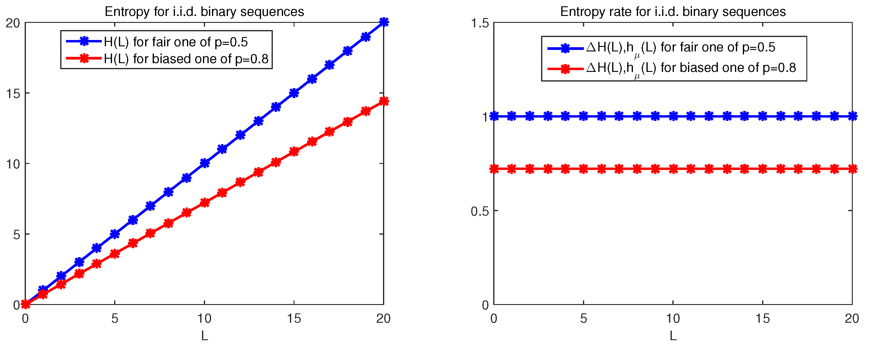
Figure 2.
Entropy (left panel) and entropy rate (right panel) curves for the period-5 sequence (red): and the period-8 sequence (blue): .
Figure 2.
Entropy (left panel) and entropy rate (right panel) curves for the period-5 sequence (red): and the period-8 sequence (blue): .

Figure 3.
Entropy (left) and entropy rate (right) curves for a Markov chain with two states (red) and a birth–death chain (blue).
Figure 3.
Entropy (left) and entropy rate (right) curves for a Markov chain with two states (red) and a birth–death chain (blue).

Figure 4.
Entropy and entropy rate curves (left); excess entropy and its logarithmic estimate (right) for a TM sequence.
Figure 4.
Entropy and entropy rate curves (left); excess entropy and its logarithmic estimate (right) for a TM sequence.

Figure 5.
Entropy (left) and excess entropy (right) curves for Ising sequences with three different interactions.
Figure 5.
Entropy (left) and excess entropy (right) curves for Ising sequences with three different interactions.

Figure 6.
Entropy (left panel) and excess entropy (right panel) curves for a stationary Gaussian sequence.
Figure 6.
Entropy (left panel) and excess entropy (right panel) curves for a stationary Gaussian sequence.
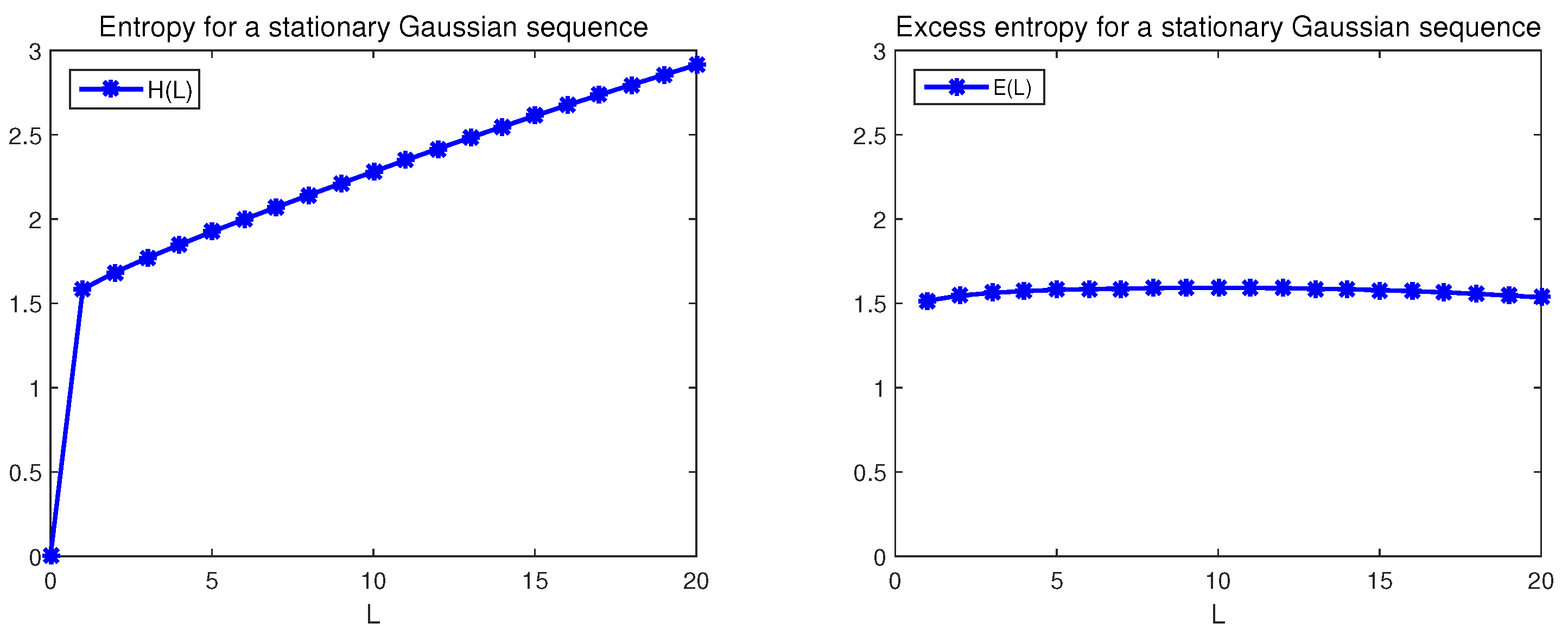
Figure 7.
Entropy for a FGN with Hurst parameters from to (left panel) and from to (right panel).

Figure 8.
Excess entropy for a FGN with Hurst parameters from to (left panel) and from to (right panel).
Figure 8.
Excess entropy for a FGN with Hurst parameters from to (left panel) and from to (right panel).

Figure 9.
Entropy (left) and excess entropy (right) for a stationary AR(2) sequence with Gaussian noise and with standard Levy noise (two parameters of and ).
Figure 9.
Entropy (left) and excess entropy (right) for a stationary AR(2) sequence with Gaussian noise and with standard Levy noise (two parameters of and ).

Figure 10.
Entropy (left), excess entropy and its logarithmic estimate (right) for another stationary AR(2) sequence with Gaussian noise and with standard Levy noise (two parameters of and ).
Figure 10.
Entropy (left), excess entropy and its logarithmic estimate (right) for another stationary AR(2) sequence with Gaussian noise and with standard Levy noise (two parameters of and ).

Figure 11.
Entropy for a AR sequence with Gaussian noise and with standard Levy noise.

Figure 12.
Entropy (left) and excess entropy (right) growth curves for hydrological data.

Figure 13.
Excess entropy growth curves and logarithmic estimates for the peak gamma-ray intensity data (left panel) and the earthquake Richter magnitude data (right panel).
Figure 13.
Excess entropy growth curves and logarithmic estimates for the peak gamma-ray intensity data (left panel) and the earthquake Richter magnitude data (right panel).

Disclaimer/Publisher’s Note: The statements, opinions and data contained in all publications are solely those of the individual author(s) and contributor(s) and not of MDPI and/or the editor(s). MDPI and/or the editor(s) disclaim responsibility for any injury to people or property resulting from any ideas, methods, instructions or products referred to in the content. |
© 2023 by the authors. Licensee MDPI, Basel, Switzerland. This article is an open access article distributed under the terms and conditions of the Creative Commons Attribution (CC BY) license (https://creativecommons.org/licenses/by/4.0/).
Share and Cite
MDPI and ACS Style
Xiang, X.; Zhou, J. An Excess Entropy Approach to Classify Long-Term and Short-Term Memory Stationary Time Series. Mathematics 2023, 11, 2448. https://doi.org/10.3390/math11112448
AMA Style
Xiang X, Zhou J. An Excess Entropy Approach to Classify Long-Term and Short-Term Memory Stationary Time Series. Mathematics. 2023; 11(11):2448. https://doi.org/10.3390/math11112448
Chicago/Turabian StyleXiang, Xuyan, and Jieming Zhou. 2023. "An Excess Entropy Approach to Classify Long-Term and Short-Term Memory Stationary Time Series" Mathematics 11, no. 11: 2448. https://doi.org/10.3390/math11112448
Note that from the first issue of 2016, this journal uses article numbers instead of page numbers. See further details here.