

Efficiency Index for Binary Classifiers: Concept, Extension, and Application

Abstract
1. Introduction
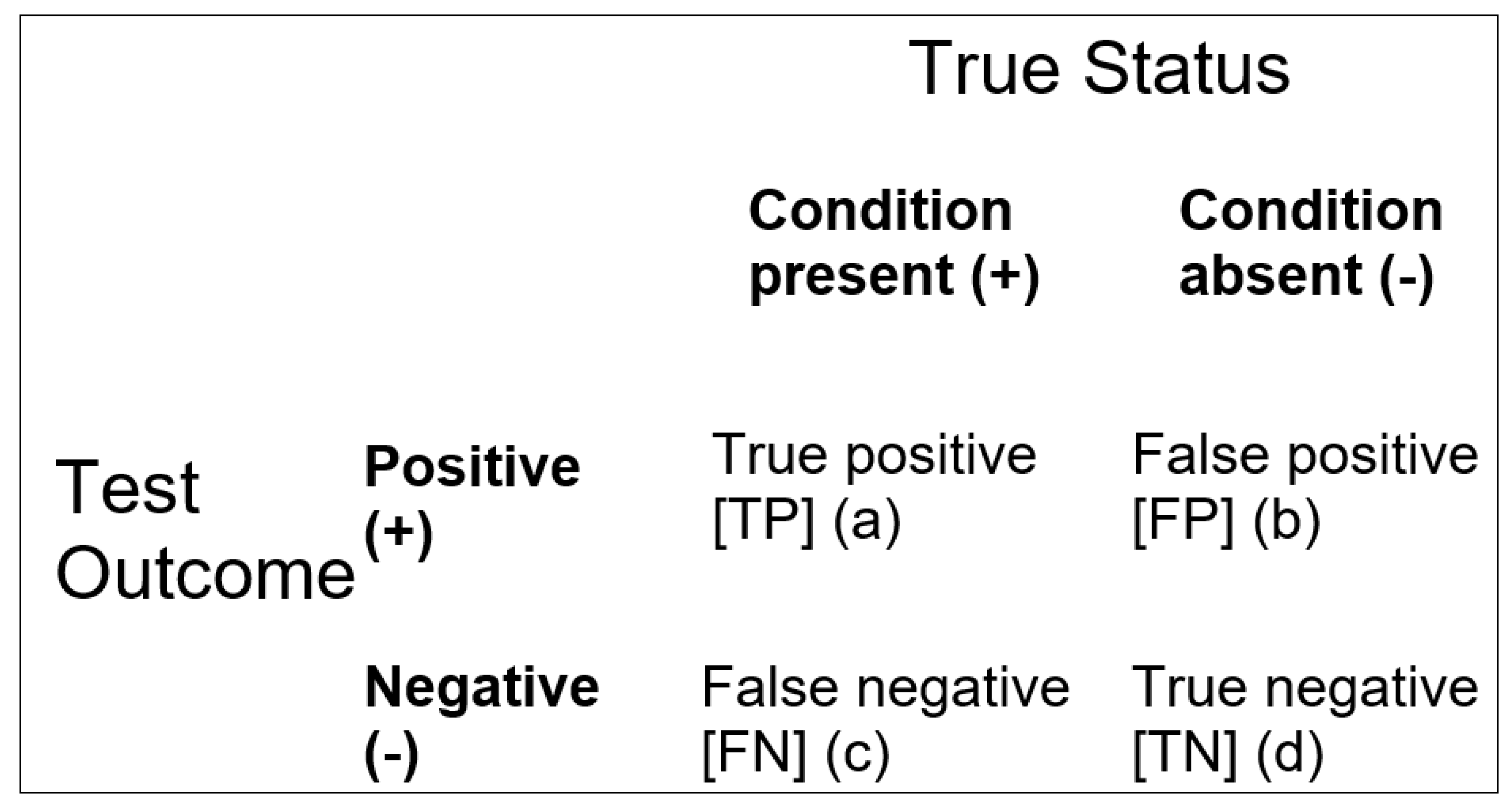
= (TP + TN)/(FP + FN)
= (a + d)/(b + c)
= (FP + FN)/(TP + TN)
= (b + c)/(a + d)
= log[Acc/(1 − Acc)]
= logit(Acc)
Inacc = (1 − Sens).P + (1 − Spec).P′

| EI Value | Qualitative Classification: Change in Probability of Diagnosis (after Jaeschke et al. [8]) | Qualitative Classification: “Effect Size” (after Rosenthal [10]) | Semi-Quantitative Classification: Approximate % Change in Probability of Diagnosis (after McGee [11]) |
|---|---|---|---|
| ≤0.1 | Very large decrease | - | - |
| 0.1 | Large decrease | - | −45 |
| 0.2 | Large decrease | - | −30 |
| 0.5 | Moderate decrease | - | −15 |
| 1.0 | 0 | ||
| ~1.5 | - | Small | - |
| 2.0 | Moderate increase | - | +15 |
| ~2.5 | - | Medium | - |
| ~4 | - | Large | - |
| 5.0 | Moderate increase | - | +30 |
| 10.0 | Large increase | - | +45 |
| ≥10.0 | Very large increase | Very large | - |
2. Methods
2.1. Participants
2.2. Analyses
2.2.1. Balanced Efficiency Index
BInacc =1 − BAcc
BInacc = [(1 − Sens) + (1 − Spec)]/2
= (Sens + Spec)/[(1 − Sens) + (1 − Spec)]
2.2.2. Balanced Level Efficiency Index
Spec = NPV.Q′/P′
Inacc = (1 − Sens).P + (1 − Spec).P′
Inacc = (1 − PPV).Q + (1 − NPV).Q′
BLInacc = 1 − BLAcc
BLInacc = [(1 − PPV) + (1 − NPV)]/2
= (PPV + NPV)/[(1 − PPV) + (1 − NPV)]
2.2.3. Quality Efficiency Index
QInacc = 1 − QAcc
QInacc = (1 − QSens).P + (1 − QSpec).P′
= (QSens + QSpec)/[(1 − QSens) + (1 − QSpec)]
2.2.4. Unbiased Efficiency Index
= Acc − (P.Q + P′.Q′)/1 − (P.Q + P′.Q′)
= UAcc/(1 − UAcc)
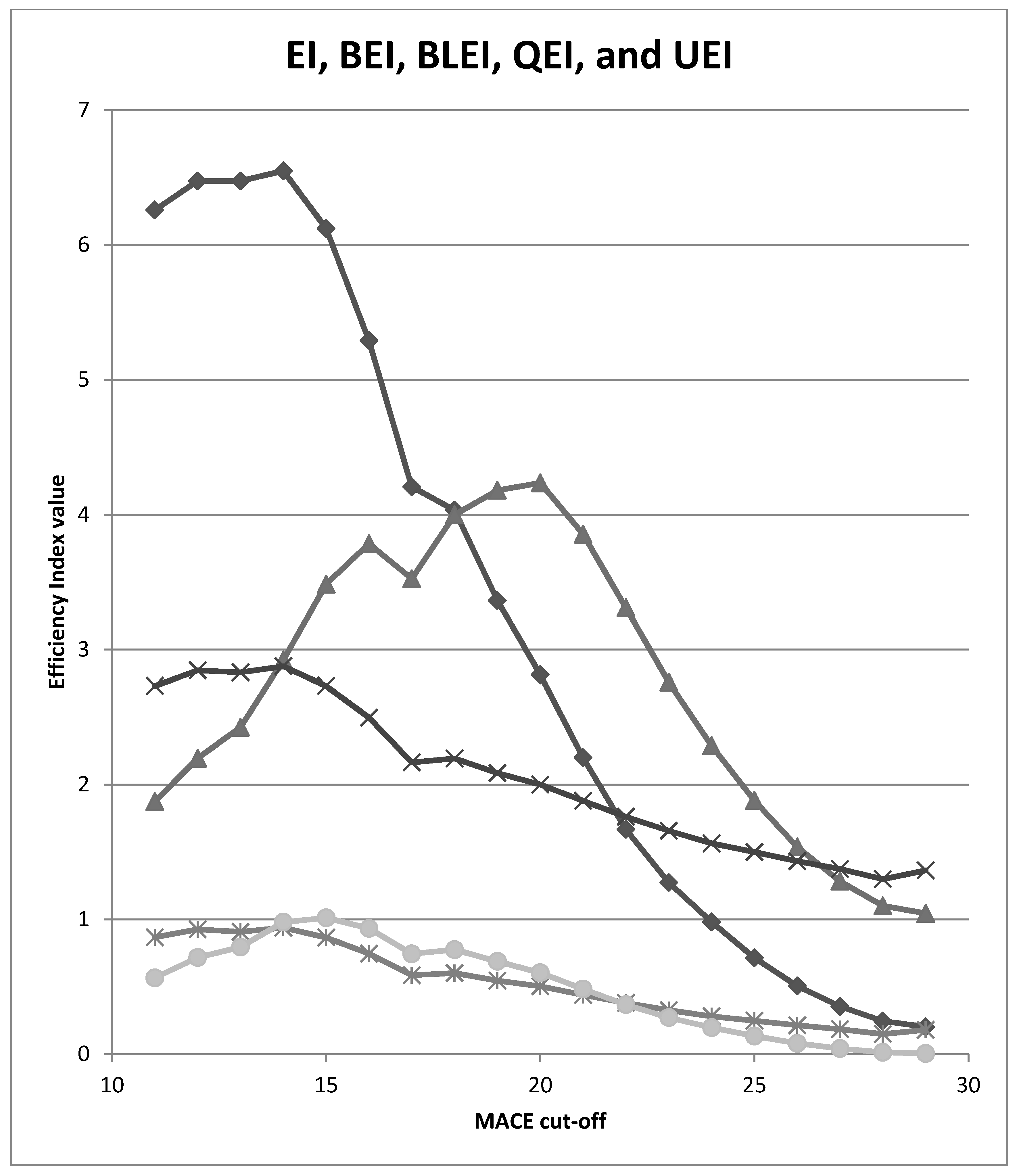
3. Results
4. Discussion
5. Limitations
6. Conclusions
Funding
Institutional Review Board Statement
Informed Consent Statement
Data Availability Statement
Conflicts of Interest
References
- Bolboacă, S.D. Medical diagnostic tests: A review of test anatomy, phases, and statistical treatment of data. Comput. Math. Methods Med. 2019, 2019, 1891569. [Google Scholar] [CrossRef] [PubMed]
- Larner, A.J. The 2 × 2 Matrix. Contingency, Confusion and the Metrics of Binary Classification; Springer: Berlin/Heidelberg, Germany, 2021. [Google Scholar]
- Larner, A.J. Communicating risk: Developing an “Efficiency Index” for dementia screening tests. Brain Sci. 2021, 11, 1473. [Google Scholar] [CrossRef] [PubMed]
- Larner, A.J. Evaluating binary classifiers: Extending the Efficiency Index. Neurodegener. Dis. Manag. 2022, 12, 185–194. [Google Scholar] [CrossRef] [PubMed]
- McNicol, D. A Primer of Signal Detection Theory; Lawrence Erlbaum Associates: Mahwah, NJ, USA, 2005. [Google Scholar]
- Kraemer, H.C. Evaluating Medical Tests. In Objective and Quantitative Guidelines; Sage: Newbery Park, CA, USA, 1992. [Google Scholar]
- Katz, D.; Baptista, J.; Azen, S.P.; Pike, M.C. Obtaining confidence intervals for the risk ratio in cohort studies. Biometrics 1978, 34, 469–474. [Google Scholar] [CrossRef]
- Jaeschke, R.; Guyatt, G.; Sackett, D.L. Users’ guide to the medical literature: III. How to use an article about a diagnostic test. B. What are the results and will they help me in caring for my patients? JAMA 1994, 271, 703–707. [Google Scholar] [CrossRef]
- Glas, A.S.; Lijmer, J.G.; Prins, M.H.; Bonsel, G.J.; Bossuyt, P.M. The diagnostic odds ratio: A single indicator of test performance. J. Clin. Epidemiol. 2003, 56, 1129–1135. [Google Scholar] [CrossRef]
- Rosenthal, J.A. Qualitative descriptors of strength of association and effect size. J. Soc. Serv. Res. 1996, 21, 37–59. [Google Scholar] [CrossRef]
- McGee, S. Simplifying likelihood ratios. J. Gen. Intern Med. 2002, 17, 647–650. [Google Scholar] [CrossRef] [PubMed]
- Larner, A.J. Cognitive screening in older people using Free-Cog and Mini-Addenbrooke’s Cognitive Examination (MACE). Preprints.org, 2023; ahead of print. [Google Scholar] [CrossRef]
- Hsieh, S.; McGrory, S.; Leslie, F.; Dawson, K.; Ahmed, S.; Butler, C.R.; Rowe, J.B.; Mioshi, E.; Hodges, J.R. The Mini-Addenbrooke’s Cognitive Examination: A new assessment tool for dementia. Dement. Geriatr. Cogn. Disord. 2015, 39, 1–11. [Google Scholar] [CrossRef] [PubMed]
- Noel-Storr, A.H.; McCleery, J.M.; Richard, E.; Ritchie, C.W.; Flicker, L.; Cullum, S.J.; Davis, D.; Quinn, T.J.; Hyde, C.; Rutjes, A.W.S.; et al. Reporting standards for studies of diagnostic test accuracy in dementia: The STARDdem Initiative. Neurology 2014, 83, 364–373. [Google Scholar] [CrossRef] [PubMed]
- Larner, A.J. MACE for diagnosis of dementia and MCI: Examining cut-offs and predictive values. Diagnostics 2019, 9, 51. [Google Scholar] [CrossRef] [PubMed]
- Larner, A.J. Accuracy of cognitive screening instruments reconsidered: Overall, balanced, or unbiased accuracy? Neurodegener. Dis. Manag. 2022, 12, 67–76. [Google Scholar] [CrossRef] [PubMed]
- Larner, A.J. Applying Kraemer’s Q (positive sign rate): Some implications for diagnostic test accuracy study results. Dement. Geriatr. Cogn. Dis. Extra 2019, 9, 389–396. [Google Scholar] [CrossRef] [PubMed]
- Garrett, C.T.; Sell, S. Summary and Perspective: Assessing Test Effectiveness–The Identification of Good Tumour Markers. In Cellular Cancer Markers; Garrett, C.T., Sell, S., Eds.; Springer: Berlin/Heidelberg, Germany, 1995; pp. 455–477. [Google Scholar]
- Carter, J.V.; Pan, J.; Rai, S.N.; Galandiuk, S. ROC-ing along: Evaluation and interpretation of receiver operating characteristic curves. Surgery 2016, 159, 1638–1645. [Google Scholar] [CrossRef] [PubMed]
- Hand, D.J.; Christen, P.; Kirielle, N. F*: An interpretable transformation of the F measure. Mach. Learn. 2021, 110, 451–456. [Google Scholar] [CrossRef] [PubMed]
- Sowjanya, A.M.; Mrudula, O. Effective treatment of imbalanced datasets in health care using modified SMOTE coupled with stacked deep learning algorithms. Appl. Nanosci. 2022, 13, 1829–1840. [Google Scholar] [CrossRef] [PubMed]
- Mbizvo, G.K.; Bennett, K.H.; Simpson, C.R.; Duncan, S.E.; Chin, R.F.M.; Larner, A.J. Using Critical Success Index or Gilbert Skill Score as composite measures of positive predictive value and sensitivity in diagnostic accuracy studies: Weather forecasting informing epilepsy research. Epilepsia, 2023; ahead of print. [Google Scholar]
- Sud, A.; Turnbull, C.; Houlston, R.S.; Horton, R.H.; Hingorani, A.D.; Tzoulaki, I.; Lucassen, A. Realistic expectations are key to realising the benefits of polygenic scores. BMJ 2023, 380, e073149. [Google Scholar] [CrossRef] [PubMed]
- Larner, A.J. Assessing cognitive screening instruments with the critical success index. Prog. Neurol. Psychiatry 2021, 25, 33–37. [Google Scholar] [CrossRef]
- Roccetti, M.; Delnevo, G.; Casini, L.; Cappiello, G. Is bigger always better? A controversial journey to the center of machine learning design, with uses and misuses of big data for predicting water meter failures. J. Big Data 2019, 6, 70. [Google Scholar] [CrossRef]


| MACE Cut-Off | EI | BEI | BLEI | QEI | UEI |
|---|---|---|---|---|---|
| ≤29/30 | 0.204 | 1.045 | 1.364 | 0.181 | 0.006 |
| ≤28/30 | 0.246 | 1.101 | 1.299 | 0.150 | 0.015 |
| ≤27/30 | 0.355 | 1.283 | 1.374 | 0.186 | 0.043 |
| ≤26/30 | 0.507 | 1.538 | 1.432 | 0.215 | 0.081 |
| ≤25/30 | 0.716 | 1.882 | 1.500 | 0.249 | 0.135 |
| ≤24/30 | 0.982 | 2.289 | 1.564 | 0.282 | 0.198 |
| ≤23/30 | 1.274 | 2.759 | 1.658 | 0.327 | 0.272 |
| ≤22/30 | 1.668 | 3.310 | 1.762 | 0.381 | 0.368 |
| ≤21/30 | 2.199 | 3.854 | 1.880 | 0.440 | 0.484 |
| ≤20/30 | 2.813 | 4.236 | 2.000 | 0.504 | 0.605 |
| ≤19/30 | 3.364 | 4.181 | 2.086 | 0.546 | 0.689 |
| ≤18/30 | 4.033 | 4.000 | 2.194 | 0.602 | 0.776 |
| ≤17/30 | 4.207 | 3.525 | 2.165 | 0.586 | 0.745 |
| ≤16/30 | 5.292 | 3.785 | 2.497 | 0.746 | 0.934 |
| ≤15/30 | 6.123 | 3.484 | 2.731 | 0.866 | 1.012 |
| ≤14/30 | 6.550 | 2.922 | 2.876 | 0.939 | 0.980 |
| ≤13/30 | 6.475 | 2.425 | 2.831 | 0.908 | 0.795 |
| ≤12/30 | 6.475 | 2.195 | 2.846 | 0.927 | 0.718 |
| ≤11/30 | 6.260 | 1.874 | 2.731 | 0.868 | 0.567 |
Disclaimer/Publisher’s Note: The statements, opinions and data contained in all publications are solely those of the individual author(s) and contributor(s) and not of MDPI and/or the editor(s). MDPI and/or the editor(s) disclaim responsibility for any injury to people or property resulting from any ideas, methods, instructions or products referred to in the content. |
© 2023 by the author. Licensee MDPI, Basel, Switzerland. This article is an open access article distributed under the terms and conditions of the Creative Commons Attribution (CC BY) license (https://creativecommons.org/licenses/by/4.0/).
Share and Cite
Larner, A.J. Efficiency Index for Binary Classifiers: Concept, Extension, and Application. Mathematics 2023, 11, 2435. https://doi.org/10.3390/math11112435
Larner AJ. Efficiency Index for Binary Classifiers: Concept, Extension, and Application. Mathematics. 2023; 11(11):2435. https://doi.org/10.3390/math11112435
Chicago/Turabian StyleLarner, Andrew J. 2023. "Efficiency Index for Binary Classifiers: Concept, Extension, and Application" Mathematics 11, no. 11: 2435. https://doi.org/10.3390/math11112435
APA StyleLarner, A. J. (2023). Efficiency Index for Binary Classifiers: Concept, Extension, and Application. Mathematics, 11(11), 2435. https://doi.org/10.3390/math11112435