The Poisson–Lindley Distribution: Some Characteristics, with Its Application to SPC

Abstract

Statistical process control (SPC) is a significant method to monitor processes and ensure quality. Control charts are the most important tools in SPC. As production processes and production parts become more complex, there is a need to design control charts using more complex distributions. One of the most important control charts to monitor the number of nonconformities in production processes is the C-chart, which uses the Poisson distribution as a quality characteristic distribution. However, to fit the Poisson distribution to the count data, equality of mean and variance should be satisfied. In some cases, such as biological and medical sciences, count data exhibit overdispersion, which means that the variance of data is greater than the mean. In such cases, we can use the Poisson–Lindley distribution instead of the Poisson distribution to model the count data. In this paper, we first discuss some important characteristics of the Poisson–Lindley distribution. Then, we present parametric and bootstrap control charts when the observations follow the Poisson–Lindley distribution and analyze their performance. Finally, we provide a simulated example and a real-world dataset to demonstrate the implementation of control charts. The results show the good performance of the proposed control charts.

1. Introduction

The quality of production is critical for achieving success in a business. There are different methods for ensuring the quality of production, and statistical process control (SPC) is one of them. SPC involves using statistical methods to monitor production processes and identify potential issues before they can affect quality. By implementing SPC, businesses can improve their quality control efforts and increase the likelihood of success. Some of the latest challenges and research areas in the field of SPC are:

• Integration with industry technologies: As more and more factories become digitized and automated, there is a need for SPC methodologies to be integrated with these new technologies. For example, using sensors to collect data in real time and feeding that data into statistical models to identify process variations and anomalies.
• Multivariate SPC: Traditional SPC techniques focus on monitoring single variables at a time, but many manufacturing processes involve multiple interconnected variables. Researchers are working on developing multivariate SPC methods that can handle these complex relationships.
• Adaptive SPC: Another area of active research is the development of adaptive SPC methods that can automatically adjust control limits in response to changes in the process.

For more studies in these fields, you can refer to [1,2,3].

The statistical tool known as the control chart, which utilizes random sampling, is widely used in the SPC to assess and monitor quality characteristics of interest collected during manufacturing processes and detect deviations from expected levels of control. As production processes and production parts become more complex, there is a need to design control charts using more complex distributions.

One of the most important control charts used to monitor the number of defective parts in production processes is the C-chart, which utilizes the Poisson distribution as a quality characteristic distribution. Situations where random events occur, such as the number of customers at a service point or the number of defects in a given material, can be modeled using the Poisson distribution. This distribution has practical applications in various fields, including telecommunications, traffic safety, and materials science. Other examples include measuring the number of meteorite collisions with a test satellite during an orbit or the number of organisms in a fluid sample.

While the Poisson distribution is commonly used for modeling independent events, it may not be suitable in cases where there is dependence between successive events. To address this issue, the negative binomial distribution can be used as an alternative to the Poisson distribution. To study more in this field, you can refer to [4,5,6]. Additionally, it is important to note that the mean and variance of count data must be equal for accurate fitting of the Poisson distribution; especially, the mean should be less than or equal to the variance. In some cases, such as in the biological and medical sciences, this condition is not fully satisfied. In such cases, we can use the Poisson–Lindley distribution $\left(PLD\right)$ instead of the Poisson distribution. Empirical and theoretical reasoning support the use of the Poisson–Lindley distribution in characterizing data from biological and medical sciences, due to its overdispersion property $(\mu <{\sigma }^2)$.

The Lindley distribution is one of the important distributions that have great potential to represent different systems consisting of complex and heterogeneous samples with high flexibility. The pdf of this distribution is given by

$$f\left(x;\theta \right)=\frac{{\theta }^2}{\left(1+\theta \right)}\left(1+x\right)e^{-\theta x} x>0 , \theta >0 ,$$

(1)

where θ is the shape parameter. In reliability and SPC, there is no need to consider the shift parameter.

The Poisson–Lindley distribution is proposed by [7] for modeling count data. This distribution emerges from the Poisson distribution, where its parameter λ conforms to the Lindley distribution [8], with a probability density function in the form of Equation (1), i.e., $X$ follows a Poisson probability density function of the form:

$$P\left(X=x|\lambda \right)=\frac{e^{-\lambda } {\lambda }^x}{x!} , \lambda >0 x=0,1,2, \dots$$

in which the parameter $\lambda$ in the Poisson distribution has a Lindley probability density function of the form:

$$\begin{array}{cc}f\left(\lambda ;\theta \right)=\frac{{\theta }^2}{\theta +1} \left(1+\lambda \right)e^{-\lambda \theta },& \lambda >0 , \theta >0 .\end{array}$$

So, we can write the probability mass function (pmf) of Poisson–Lindley distribution as follows:

$$P\left(X=x,\lambda \right)=P\left(X=x|\lambda \right)f\left(\lambda \right)$$

$$p\left(x\right)=P\left(X=x\right)={\displaystyle {\int }_0^{\infty }}P\left(X=x|\lambda \right)f\left(\lambda \right)d\lambda ={\displaystyle {\int }_0^{\infty }}\frac{e^{-\lambda } {\lambda }^x}{x!}\frac{{\theta }^2}{\left(\theta +1\right)}\left(1+\lambda \right)e^{-\theta \lambda }d\lambda .$$

Therefore, the pmf of the PLD is equals to:

$$p\left(x\right)=\frac{{\theta }^2\left(\theta +x+2\right)}{{\left(1+\theta \right)}^{x+3}}, x=0,1,2,\dots \theta >0 .$$

(2)

The cumulative distribution function (cdf) of Poisson–Lindley distribution is as follows:

$$\begin{array}{ll}F\left(x\right)=P\left(X\le x\right)& =1-P\left(X>x+1\right)=1-{\displaystyle \sum _{t=x+1}^{\infty }}{\displaystyle \underset{0}{\overset{\infty }{\int }}}P\left(X=t|\lambda \right)f\left(\lambda \right)d\lambda \\ & =1-{\displaystyle \sum _{t=x+1}^{\infty }}{\displaystyle \underset{0}{\overset{\infty }{\int }}}\frac{e^{-\lambda } {\lambda }^t}{t!}\frac{{\theta }^2}{\left(\theta +1\right)}\left(1+\lambda \right)e^{-\theta \lambda }d\lambda \end{array}$$

$$F\left(x\right)=1-\frac{{\theta }^2+3\theta +1+\theta x}{{(\theta +1)}^{x+3}} ,x=0,1,2,\dots \theta >0 .$$

(3)

There exist several generalizations of the Poisson–Lindley distribution. The generalized Poisson–Lindley distribution was introduced by [9], while the two-parameter Poisson–Lindley distribution was introduced by [10] using a combination of a Poisson distribution with the two-parameter Lindley distribution. The complementary Poisson–Lindley class of distributions was introduced by [11], and the bivariate Poisson–Lindley distribution was introduced by [12]. Additionally, the size-biased two-parameter Poisson–Lindley distribution was introduced by [13], and the three-parameter Poisson–Lindley distribution was introduced by [14].

The Maximum Likelihood and Method of Moments estimations of the Poisson–Lindley distribution are presented in [7], where their consistency and asymptotic behavior are also investigated in [15].

To track a quality characteristic $X$ at pre-defined targets ${\mu }_0$ and ${\sigma }_0$ in industrial processes, practitioners often employ Shewhart control charts with 3-sigma control limits. For a comprehensive overview of these charts, one may refer to [16].

Given the non-availability of an analytical expression for the $MLE$ of the shape parameter in Poisson–Lindley processes, inferring its sampling distribution can be challenging. This limitation is overcome by using bootstrap control charts, which offer a reliable way of monitoring these processes. Details about the bootstrap methodology can be found in [17]. Examples of bootstrap control charts can be found in [18,19,20,21,22,23,24].

So far, no control chart has been presented for data that are over-dispersed. Therefore, considering the importance of such data, in this paper we have presented control charts for them using Poisson–Lindley distribution. For this purpose, in Section 2, we review some of the characteristics of the $PLD$. Control charts for the data to which the $PLD$ is fitted are presented in Section 3. Section 4 includes numerical results and simulation for the implementation of the control charts. Finally, the discussion and conclusions are presented in Section 5.

2. Some of the Characteristics of the $\mathit{P}\mathit{L}\mathit{D}$

In this section, we will first explain some characteristics of the distribution, such as the graph of the probability mass function, in addition to the mean, variance, moment-generating function, skewness and kurtosis. Then, we will talk about generating random numbers from $PLD$ and estimating the parameter of the $PLD$.

Figure 1 illustrates the pmf for the Poisson–Lindley distribution in Equation (2), showing how it changes at different values of $\theta$.

2.1. Moments

Moments of the $PLD$ are calculated using the following relation:

$$E\left(X^k\right)={\displaystyle \sum }_{x=0}^{\infty }{x}^{k}P\left(X=x\right)={\displaystyle \sum }_{x=0}^{\infty }{x}^k\frac{{\theta }^2\left[\theta +x+2\right]}{{\left(1+\theta \right)}^{x+3}}$$

$$\begin{array}{l}=\frac{{\theta }^2}{{\left(1+\theta \right)}^3}[\frac{\left(\theta +2\right)}{{\theta }^{k+1}}{\displaystyle \sum _{i=1}^k}\left\{\frac{1}{{\left(1+\theta \right)}^{k-i}}{\displaystyle \sum _{j=0}^i}\frac{{\left(-1\right)}^j\left(k+1\right)!{\left(i-j\right)}^k}{j!\left(k+1-j\right)!}\right\}\\ +\frac{1}{{\theta }^{k+2}}{\displaystyle \sum _{i=1}^k}\left\{\frac{1}{{\left(1+\theta \right)}^{k+1-i}}{\displaystyle \sum _{j=0}^i}\frac{{\left(-1\right)}^j\left(k+2\right)!{\left(i-j\right)}^{k+1}}{j!\left(k+2-j\right)!}\right\}].\end{array}$$

Using the above relation, we can obtain:

$$\mu =E\left(X\right)=\frac{\left(\theta +2\right)}{\theta \left(\theta +1\right)}$$

(4)

$$E\left(X^2\right)=\frac{{\theta }^2+4\theta +6}{\left(\theta +1\right){\theta }^2} ,$$

which implies that

$${\sigma }^2=Var\left(X\right)=\frac{{\theta }^3+4{\theta }^2+6\theta +2}{{\theta }^2{(\theta +1)}^2} .$$

(5)

Note that ${\sigma }^2=\mu \left[1+\frac{{\theta }^2+4\theta +2}{\theta \left(\theta +1\right)\left(\theta +2\right)}\right]>\mu$, indicating that the Poisson–Lindley distribution is over-dispersed.

Also, the third and fourth central moments are:

$$E\left(X^3\right)=\frac{\left({\theta }^2+6\theta +12\right)\left(\theta +2\right)}{\left(\theta +1\right){\theta }^3}$$

$$E\left(X^4\right)=\frac{{\theta }^4+16{\theta }^3+78{\theta }^2+168\theta +120}{\left(\theta +1\right){\theta }^4} .$$

So, the skewness and kurtosis of the $PLD$ are given by the following relations, respectively:

$$skewness=\frac{2{(\theta +1)}^4\left(\theta +2\right)-{\theta }^3\left(\theta +2\right)\left(\theta +3\right)}{{\left[2{(\theta +1)}^3-{\theta }^2\left(\theta +2\right)\right]}^{3/2}}$$

and

$$kurtosis=3+\frac{2{(\theta +1)}^5\left[{(\theta +3)}^2-3\right]-{\theta }^4\left(\theta +2\right)\left[{(\theta +4)}^2-3\right]}{{\left[2{(\theta +1)}^3-{\theta }^2\left(\theta +2\right)\right]}^2}.$$

2.2. Moment Generating Function and Probability Generating Function

The moment-generating function of a $PLD$ is given by:

$$M_X\left(t\right)=E\left(e^{tX}\right)=\frac{\left(\theta -e^t+2\right){\theta }^2}{\left(\theta +1\right){\left(\theta +1-e^t\right)}^2} .$$

Also, the moment generating function of the sample mean of a $PLD$ is equal to:

$$M_{\overline{X}}\left(t\right)=E\left(e^{t\overline{X}}\right)={\displaystyle {\prod }_{i=1}^n}{M}_{X_i}\left(\frac{t}{n}\right)={\left(M_{X_i}\left(\frac{t}{n}\right)\right)}^n={\left(\frac{\left(\theta -e^{\frac{t}{n}}+2\right){\theta }^2}{\left(\theta +1\right){\left(\theta +1-e^{\frac{t}{n}}\right)}^2}\right)}^n.$$

The probability generating function of the $PLD$ is given by:

$$p_x=E\left(t^X\right)=\frac{\left(\theta -t+2\right){\theta }^2}{\left(\theta +1\right){\left(-\theta +t-1\right)}^2} .$$

2.3. Generating Random Numbers from PLD

In this section, we discuss how to generate random numbers from the Poisson–Lindley distribution. One reliable method for generating a random variable x that conforms to the $PLD$ is to generate the parameter $\lambda$ from the Lindley distribution (with $\theta$ as its parameter) and then generate $x$ from the Poisson distribution using $\lambda$ as its parameter. To generate $\lambda$, notice that the Lindley distribution can be expressed as the combination of an Exponential distribution and a gamma distribution as follows:

$$\begin{array}{cc}w\left(\lambda ;\theta \right)=p{w}_1\left(\lambda ;\theta \right)+\left(1-p\right)w_2\left(\lambda ;\theta \right),& \lambda >0, \theta >0\end{array},$$

where

$$\begin{array}{ccc}p=\frac{\theta }{\theta +1},& w_1\left(\lambda ;\theta \right)=\theta e^{-\theta \lambda }& \begin{array}{cc}, & w_2\left(\lambda ;\theta \right)={\theta }^2\lambda e^{-\theta \lambda }\end{array}\end{array} ,$$

and, $w_1\left(\lambda ;\theta \right)$ and $w_2\left(\lambda ;\theta \right)$ are the probability density functions of the exponential distribution with parameter $\theta$ and the gamma distribution with parameters 2 and $\theta$, respectively.

Now we can generate a random number $x$ from the $PLD$ using the following Algorithm 1.

Algorithm 1: Generating a random number from the $PLD$

Step 1: Generate $\lambda$ from a Lindley distribution with parameter $\theta$ as follows:

(i) Generate $u$ from a $Uniform \left(0, 1\right)$ distribution.

(ii) If $u\le p=\frac{\theta }{\left(\theta +1\right)}$, let $\lambda =y_1$; otherwise, let $\lambda =y_1+y_2$, where $y_1$ and $y_2$ are random numbers generated from an $Exp\left(\theta \right)$ distribution.

Step 2: Generate $x$ from a Poisson distribution with parameter $\lambda$.

2.4. Estimation of the Parameter of the $PLD$

Let $x_1,x_2,\dots ,x_n$ be $n$ observations from a $PLD$ with parameter $\theta$.

2.4.1. Method of Moment Estimation

The method of moment $\left(MoM\right)$ estimation of $\theta$, given by [7], is as follows:

$$\tilde{\theta }=\frac{-\left(\overline{x}-1\right)+\sqrt{{\left(\overline{x}-1\right)}^2+8\overline{x}}}{2\overline{x}} .$$

(6)

Ref. [15] has proven that

$$\sqrt{n}(\tilde{\theta }-\theta )\stackrel{d}{\to }N\left(0,v^2\left(\theta \right)\right)$$

where,

$$v^2\left(\theta \right)=\frac{{\theta }^2(\theta +1{)}^2({\theta }^3+4{\theta }^2+6\theta +2)}{{\theta }^2+4\theta +2}.$$

Based on this result, an asymptotic $100\left(1-\alpha \right)\%$ confidence interval for $\theta$ is presented as follows

$$\tilde{\theta }\pm Z_{\alpha /2}\frac{v\left(\tilde{\theta }\right)}{\sqrt{n}}.$$

2.4.2. Maximum Likelihood Estimation

The likelihood function of observations $x_1,x_2,\dots ,x_n$ from pmf of Equation (2) is equal to:

$$\begin{array}{l}L\left(\theta \right)=L\left(\theta ;x_1,x_2,\dots ,x_n\right)={\displaystyle \prod _{i=1}^n}P\left(X_i=x_i\right)={\displaystyle \prod _{i=1}^n}\frac{{\theta }^2\left(\theta +x_i+2\right)}{{\left(1+\theta \right)}^{x_i+3}}\\ =\frac{{\theta }^2}{{\left(1+\theta \right)}^3}{\displaystyle \prod _{i=1}^n}\frac{\left(\theta +x_i+2\right)}{{\left(1+\theta \right)}^{x_i}}={\left(\frac{{\theta }^2}{{\left(1+\theta \right)}^3}\right)}^n\frac{\prod _{i=1}^n\left(\theta +x_i+2\right)}{\prod _{i=1}^n{\left(1+\theta \right)}^{x_i}}\\ =\frac{{\theta }^{2n}}{{\left(1+\theta \right)}^{3n}}\frac{\prod _{i=1}^n\left(\theta +x_i+2\right)}{{\left(1+\theta \right)}^{\sum _{i=1}^n{x}_i}}\\ =\frac{{\theta }^{2n}}{{\left(1+\theta \right)}^{3n}}\frac{1}{{\left(1+\theta \right)}^{n\overline{x}}}{\displaystyle \prod _{i=1}^n}\left(\theta +x_i+2\right).\end{array}$$

Therefore, $l=logL\left(\theta \right)=2nlog\theta -3nlog\left(1+\theta \right)-n\overline{x}log\left(1+\theta \right)+\sum _{i=1}^{n}log\left(\theta +x_i+2\right)$, and the maximum likelihood $\left(ML\right)$ estimate, $\widehat{\theta }$ of $\theta$, is the solution of the nonlinear equation:

$$\frac{\partial l}{\partial \theta }=\frac{2n}{\theta }-\frac{n\left(\overline{x}+3\right)}{\theta +1}+\sum _{i=1}^n\frac{1}{x_i+\theta +2}=0.$$

(7)

Equation (7) has a unique solution for all $n$, but it does not have a closed-form solution, and must be calculated with numeric methods [15]. Additionally,

$$\sqrt{n}\left(\widehat{\theta }-\theta \right)\stackrel{d}{\to }N\left(0,I^{-1}\left(\theta \right)\right),$$

where

$$I\left(\theta \right)=\frac{2}{{\theta }^2}-\frac{3{\theta }^2+4\theta +2}{\theta {\left(\theta +1\right)}^3}+\frac{{\theta }^2}{{\left(\theta +1\right)}^2}{\displaystyle \underset{0}{\overset{1}{\int }}}\frac{t^{\theta +1}}{\theta +1-t}dt$$

is Fisher’s information about $\theta$. Based on this, an asymptotic $100\left(1-\alpha \right)\%$ confidence interval for $\theta$ is presented as follows:

$$\widehat{\theta }\pm Z_{\alpha /2}\frac{I^{-1/2}\left(\widehat{\theta }\right)}{\sqrt{n}}.$$

3. Control Charts for Poisson–Lindley Processes

When observing nonconformities in an inspection unit for a particular type of product, it is important to note that although the inspection unit can be a single unit of the product, it is not always the case. The inspection unit can also be a group of products that are easy to maintain records and information about. This group may consist of five, ten, or any other desired number of units of the product. In this section, we will introduce control charts for nonconformities of inspection units based on the Poisson–Lindley distribution.

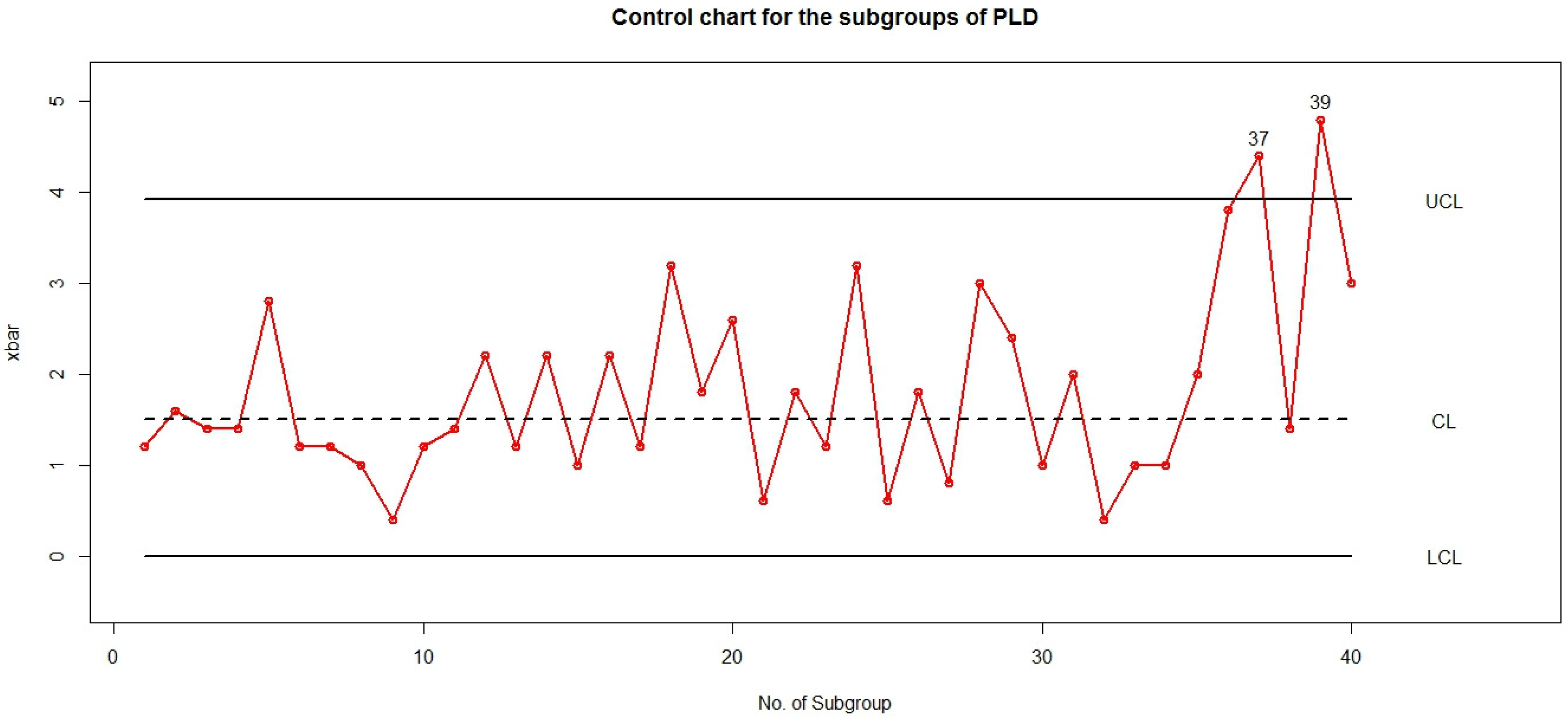
3.1. Control Charts When the Parameter Is Known

Assume that nonconformities occur in the inspection unit based on the Poisson–Lindley distribution with parameter $\theta$ and pmf of Equation (2), where $x$ is the number of nonconformities, a Shewhart-type control chart for nonconformities in the inspection unit with three sigma limits, can be defined according to Equations (4) and (5), as follows:

$$\begin{array}{c}UCL=\frac{\left(\theta +2\right)}{\theta \left(\theta +1\right)}+3\sqrt{\frac{{\theta }^3+4{\theta }^2+6\theta +2}{{\theta }^2(\theta +1{)}^2}}\\ CL=\frac{\left(\theta +2\right)}{\theta \left(\theta +1\right)}\\ LCL=\frac{\left(\theta +2\right)}{\theta \left(\theta +1\right)}-3\sqrt{\frac{{\theta }^3+4{\theta }^2+6\theta +2}{{\theta }^2(\theta +1{)}^2}}.\end{array}$$

(8)

If the calculated value for $LCL$ is negative, it should be set equal to zero.

Additionally, considering that $E\left(\overline{X}\right)=\mu$ and $Var\left(\overline{X}\right)=\frac{{\sigma }^2}{n}$, the $\overline{X}$ control chart based on $PLD$ can be defined as follows:

$$\begin{array}{c}UCL=\frac{\left(\theta +2\right)}{\theta \left(\theta +1\right)}+3\sqrt{\frac{{\theta }^3+4{\theta }^2+6\theta +2}{n{\theta }^2(\theta +1{)}^2}}\\ CL=\frac{\left(\theta +2\right)}{\theta \left(\theta +1\right)}\\ LCL=\frac{\left(\theta +2\right)}{\theta \left(\theta +1\right)}-3\sqrt{\frac{{\theta }^3+4{\theta }^2+6\theta +2}{n{\theta }^2(\theta +1{)}^2}}.\end{array}$$

(9)

Again, if the calculated value for $LCL$ is negative, set it equal to zero.

3.2. Control Charts When the Parameter Is Unknown

In many cases, the distribution parameter is unknown in practice. In such cases, the control chart for individual observations would be defined as follows:

Let $x_1,x_2,\dots ,x_m$ be our observations assumed to have a $PLD$ with parameter $\theta$, and we want to define a control chart for them. Then, the $LCL$, $CL$, and $UCL$ values can be computed from Equation (8), where $\theta$ is replaced by its $MoM$ or $ML$ estimates, i.e., $\tilde{\theta }$ or $\widehat{\theta }$ of Equations (6) or (7), respectively. For instance, $\overline{x}=\frac{\sum _{i=1}^m{x}_i}{m}$.

Suppose we have m subgroups of size $n$ and want to draw $\overline{X}$ control chart. In that case, let $x_{\mathrm{i}1},x_{\mathrm{i}2},\dots ,x_{in}$, $i=\mathrm{1,2},\dots ,m$ be $i$th subgroup sample of size $n$ that has a $PLD$ with parameter $\theta$. Let ${\overline{x}}_i=\frac{\sum _{j=1}^n{x}_{ij}}{n}$ and $\overline{\overline{x}}=\frac{{\sum }_{i=1}^m{\overline{x}}_i}{m}$. Then, the $LCL$, $CL$, and $UCL$ values can be computed from Equation (9), where $\theta$ is replaced by its $MoM$ estimate, $\tilde{\theta }$ of Equation (6). Instead of using $\overline{x}$, one must use $\overline{\overline{x}}$ to compute $\tilde{\theta }$. Additionally, the $LCL$, $CL$, and $UCL$ values can be computed from Equation (9), where $\theta$ is replaced by its $ML$ estimate, $\widehat{\theta }$ of Equation (7). In this case, one must use all $mn$ observations together to compute $\widehat{\theta }$.

The main criterion for evaluating control charts is the average run length $\left(ARL\right)$. To calculate this value in an $\overline{X}$ control chart, we need to know the $\overline{X}$ distribution in both in-control and out-of-control states. We attempted to obtain the $\overline{X}$ distribution by assuming that $X_1,X_2,\dots ,X_{\mathrm{n}}$ follow a Poisson–Lindley distribution with parameter $\theta$. However, even after calculating the moment-generating function of $\overline{X}$ in Section 2.2, we were unable to identify its distribution. Therefore, we had to resort to using the bootstrap technique for this purpose.

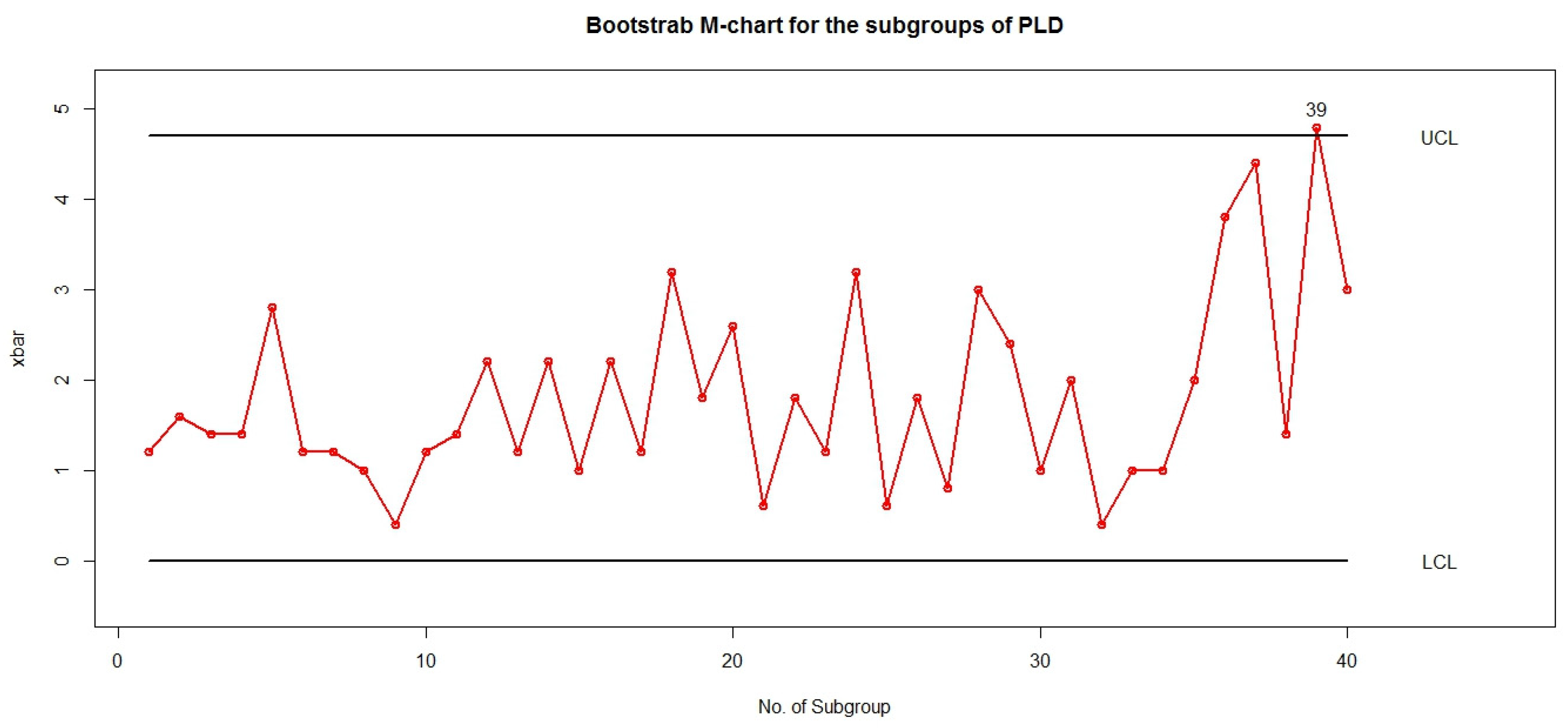
3.3. Bootstrap Control Charts

In Poisson–Lindley processes, we do not have an explicit formula for the $MLE$ estimator of the parameter. Since closed-form expressions for their sampling distribution and key statistics such as the sample mean and standard deviation are not available, analyzing these data sets can be challenging. Therefore, to monitor Poisson–Lindley processes, bootstrap control charts are very useful. As seen in Figure 1, the Poisson–Lindley distribution is a skewed distribution, especially for large values of $\theta$, where the amount of skewness is very high. In the case of skewed distributions, several studies indicate that bootstrap control charts generally outperform Shewhart control charts (see [25,26,27]). Therefore, in this section, we introduce bootstrap control charts for the Poisson–Lindley distribution.

To construct a bootstrap control chart, we rely solely on the sample data to estimate the parameter estimator’s sampling distribution and appropriate control limits. Therefore, conforming to the traditional assumptions associated with control charts—i.e., a stable process and independent, identically distributed subgroup observations—is sufficient. The following Algorithm 2, similar to the ones proposed in [19,20,21], can be used to implement bootstrap control charts for subgroup samples of size $n$, to monitor the process mean value (M-chart) and the process standard deviation (S-chart) of a Poisson–Lindley distribution, respectively.

Algorithm 2: Computing the Bootstrap M and S control charts

Phase I: Estimation and computation of the control limits

When the process is in a state of in-control and stability, observe $m$ (for example, 25 or 30) random samples of size $n$. It should be assumed that the observations are independent and identically distributed according to a Poisson–Lindley distribution with parameter $\theta$ To obtain the maximum likelihood $\left(ML\right)$ estimate of $\theta$, use Equation (7) and apply it to the pooled sample of size $m\times n$. Using Algorithm 1, generate a parametric bootstrap sample of size $n$, $(x_1^{*},\dots ,x_n^{*})$ from a Poisson–Lindley distribution, with the $ML$ estimate obtained in Step 2 used as the distribution parameter. To monitor the mean value of the process, $\mu$ (M-chart), use the sample mean $\widehat{\mu }={\overline{x}}^{*}$ derived from the bootstrap subgroup obtained in Step 3. Similarly, to monitor the process standard deviation, $\sigma$ (S-chart), use the sample standard deviation $\widehat{\sigma }=s^{*}$ computed from the bootstrap subgroup in Step 3. To obtain B bootstrap estimates of the parameter of interest (either ${\overline{x}}^{*}$ or $s^{*}$), repeat Steps 3–4 a considerable number of times, such as B = 10,000 iterations. Let that $\gamma$ denote the intended false alarm rate (FAR) for the chart. To create the bootstrap M-chart, use the B bootstrap estimations obtained in Step 5 and set the lower control limit $\left(LCL\right)$ to the ${(\gamma /2)}^{\mathrm{t}\mathrm{h}}$ quantile of the distribution of ${\widehat{\mu }}^{\mathrm{*}}$ and the upper control limit $\left(UCL\right)$ to the ${(1-\gamma /2)}^{\mathrm{t}\mathrm{h}}$ quantile of the distribution of ${\widehat{\mu }}^{\mathrm{*}}$. For the bootstrap S-chart, set the $UCL$ to the ${(1-\gamma )}^{\mathrm{t}\mathrm{h}}$ quantile of the distribution of ${\widehat{\sigma }}^{\mathrm{*}}$. Note, that in statistical quality control, a lower standard deviation indicates better quality, and reducing the standard deviation does not cause the system to go out of control. Therefore, the $LCL$ for S-chart is considered equal to 0.

Phase II: Monitoring of process

7. Obtain subgroup samples of size n from the process at fixed time intervals of h hours (For example, once every hour or every half an hour). For each subgroup, compute the estimated values of $\overline{x}$ and $s$. 8. Decision: The M-chart signals that the process mean may be out of control when $\overline{x}$ falls below the $LCL$ or above the $UCL$. Conversely, if $\overline{x}$ falls between the $LCL$ and $UCL$, the mean of the process is deemed to be in control. Meanwhile, the S-chart indicates that the variance of the process could be out of control if s falls above the $UCL$; otherwise, if $s$ falls below the $UCL$, the variance of the process is assumed to be in control.

Repeating Steps 1 to 6 of Algorithm 2 numerous times (e.g., $k=30$ times) is necessary in order to obtain an average value for the control limits ($UCL$ and $LCL$) and their associated variances. This approach provides insights into the robustness of the bootstrap control limits.

The present investigation employed Algorithm 2 to create bootstrap M-charts and S-charts for subgroups of size $n=5$. These control charts were used to monitor the process mean and standard deviation values of a Poisson–Lindley process at target values of ${\mu }_0$, and ${\sigma }_0$ respectively. Without loss of generality, we assume $\theta =1$ (or equivalently ${\mu }_0=1.5$, and ${\sigma }_0^2=3.25$). Assuming a false alarm rate (FAR) of $\gamma =0.0027$, there is an expected in-control average run length (${ARL}_0$) of approximately 370.4. In the implementation of bootstrap control charts, we used $m=25$ subgroups, each containing $n=5$ observations during Phase I.

The performance of the bootstrap M and S control charts in identifying changes in the process mean and standard deviation was evaluated based on the average run lengths $\left(ARLs\right)$. Various levels of change were considered to assess the charts’ efficacy. In scenarios where the process shifts from the in-control state to an out-of-control state, it is assumed that the mean of the process shifts from $\mu ={\mu }_0$ to $\mu ={\mu }_0+\delta {\sigma }_0$, and/or the standard deviation of the process changes from ${\sigma }_0$ to $\xi {\sigma }_0$. Since variance reduction is not desired in SPC, it is assumed that $\xi >1$. Additionally, for the negative values of $\delta$, notice that because in the $PLD$, ${\sigma }^2>\mu$, and $\mu >0$, $\delta$ cannot be a very small number. Because, in this case, the number calculated for $LCL$ will be a negative value that should be considered equal to 0. Additionally, since our data are of counting type, none of them will be less than $LCL$. Consequently, $ARL$ and $SDRL$ cannot be calculated in this situation.

We set the $\delta$ values for the M-chart equal to 0 (no change in the mean of the process, to check the false alarm rate), 0.25, 0.5, 0.75 (to investigate positive low shift values in the mean of the process), 1, 1.25, 1.5 (to investigate positive moderate shift values in the mean), 2, 2.25, and 2.5 (to investigate positive high shift values in the mean). Additionally, we investigated negative shifts in the mean by setting $\delta$ equal to −0.2, −0.04, −0.6, and −0.8. We did not include any values less than −0.8 because the $LCL$ for M-chart would be negative.

For the S-chart, we put the $\xi$ values equal to 1 (no change in variance of the process, to check for false alarms), 1.1, 1.2, 1.3, and 1.4 (to check for small changes in variance), 1.5, 1.6, 1.7, 1.8, and 1.9 (to examine moderate changes in variance), and 2, 2.25, and 2.5 (to examine large changes in variance).

For each value of $\delta$ and $\xi$, we set $m=25$, $n=5$, $B=\mathrm{10,000}$, and $\gamma =0.0027$. Then, we repeated steps 1 to 6 of Algorithm 2, $k=30$ times. The results are presented in

Table 1. $ARL$ and $SDRL$ of the bootstrap $M$ and $S$ charts for subgroups of size $n=5$.

M-Chart			S-Chart
δ	$\mathit{A}\mathit{R}\mathit{L}$	$\mathit{S}\mathit{D}\mathit{R}\mathit{L}$	ξ	$\mathit{A}\mathit{R}\mathit{L}$	$\mathit{S}\mathit{D}\mathit{R}\mathit{L}$
0	370.61	371.72	1	370.71	369.83
0.25	182.43	185.64	1.1	156.78	162.49
0.5	51.31	58.42	1.2	52.36	55.74
0.75	18.67	22.96	1.3	26.35	28.47
1	8.23	7.32	1.4	14.18	14.93
1.25	4.15	3.97	1.5	8.32	7.64
1.5	2.34	1.83	1.6	5.92	5.76
1.75	1.76	1.28	1.7	4.56	3.97
2	1.22	0.63	1.8	3.47	3.16
2.25	1.14	0.42	1.9	2.95	2.48
2.5	1.03	0.24	2	2.52	2.23
−0.2	132.4	136.3	2.25	2.18	1.34
−0.4	43.6	44.7	2.5	1.50	1.12
−0.6	8.8	8.2
−0.8	2.2	1.9

.

Table 1 presents the $ARL$ associated with the $SDRL$ values of the bootstrap M-chart and S-chart for different values of $\delta$ and $\xi$. The table indicates that the performance of both the bootstrap M and S control charts is outstanding, even when minor changes are taken into account. For example, if the mean of a Poisson−Lindley process with parameter $\theta =1$ increases by $1.5\sigma$ $(\delta =1.5)$, the bootstrap M-chart will detect this shift on average after 2.34 sampling times with a standard deviation of 1.83. Additionally, if the standard deviation of a Poisson−Lindley process with parameter $\theta =1$ is doubled ($\xi =2$), the bootstrap S-chart will detect this change on average after 2.52 samplings with a standard deviation of 2.23. Furthermore, in the M-Chart, when the process is in control $(\delta =0)$, $ARL$ is equal to 370.61. This indicates that on average, for every 370.61 samples, the M-Chart has one false alarm. Similarly, in the S-Chart, when the process is in control ($\xi =1$), the $ARL$ is 370.71.

In general, in both bootstrap M and S control charts, as the magnitude of the change increases, there is a rapid reduction in the $ARL$ and SDRL values.

3.4. Process Capability Analysis Using the Proposed Control Charts

The common way to express process capability is to use the process efficiency ratio ($PCR$ or $C_p$). This ratio is calculated in Shewhart-type control charts for a quality characteristic as follows:

$$C_p=PCR=\frac{USL-LSL}{6\sigma }$$

(10)

where, USL and LSL are upper and lower specification limits, respectively, which must be specified by the process design engineers.

Since the control charts introduced in Section 3.1 and Section 3.2 are also of the Shewhart type, $C_p$ is calculated for them using Equation (10), where $\sigma$ is derived from the square root of ${\sigma }^2$ in Equation (5). In the case of an unknown parameter, $\sigma$ can be estimated using either $\tilde{\theta }$ or $\widehat{\theta }$ from Equations (6) and (7), respectively.

Another process capability ratio that takes process centering into account is $C_{p_k}$, which is calculated for a quality characteristic in Shewhart-type control charts as follows:

$$C_{p_k}=\mathrm{m}\mathrm{i}\mathrm{n}(C_{p_u},C_{p_l})$$

(11)

where, $C_{p_u}=\frac{USL-\mu }{3\sigma }$ and $C_{p_l}=\frac{\mu -LSL}{3\sigma }$.

For the control charts introduced in Section 3.1 and Section 3.2, $\mu$ is calculated using Equation (4), and $\sigma$ is derived from the square root of ${\sigma }^2$ in Equation (5). In the case of an unknown parameter, it can be estimated using either $\tilde{\theta }$ or $\widehat{\theta }$.

For bootstrap control charts, $C_p$ can be calculated from the following equation:

$$C_p=PCR=\frac{USL-LSL}{UCL-LCL}$$

(12)

where the process design engineers must specify the USL and LSL values again. For the bootstrap M-chart, the $LCL$ is calculated as the $(\gamma /2)$th quantile of the distribution of ${\widehat{\mu }}^{\mathrm{*}}$ and the $UCL$ is calculated as the $(1-\frac{\gamma }{2})$th quantile of the distribution of ${\widehat{\mu }}^{\mathrm{*}}$. Additionally, for the bootstrap S-chart, the $UCL$ is calculated as the $(1-\gamma )$th quantile of the distribution of ${\widehat{\sigma }}^{\mathrm{*}}$, while the $LCL$ is set to zero. These values must be calculated using Algorithm 2.

For the bootstrap M-Chart, $C_{p_k}$ is calculated using Equation (11), where $C_{p_u}=\frac{USL-mean\left({\widehat{\mu }}^{\mathrm{*}}\right)}{3sd\left({\widehat{\mu }}^{\mathrm{*}}\right)}$ and $C_{p_l}=\frac{mean\left({\widehat{\mu }}^{*}\right)-LSL}{3sd\left({\widehat{\mu }}^{*}\right)}$. The $LCL$ is calculated as the $(\gamma /2)$th quantile of the distribution of ${\widehat{\mu }}^{\mathrm{*}}$, while the $UCL$ is calculated as the $(1-\frac{\gamma }{2})th$ quantile of the distribution of ${\widehat{\mu }}^{\mathrm{*}}$. Here, $mean\left({\widehat{\mu }}^{*}\right)$ and $sd\left({\widehat{\mu }}^{*}\right)$ are the mean and standard deviation of the distribution of ${\widehat{\mu }}^{\mathrm{*}}$, respectively. Since the bootstrap S-chart is a one-limit control chart, its $C_{p_k}$ value is equal to $C_{p_u}=\frac{USL-mean\left({\widehat{\sigma }}^{*}\right)}{3sd\left({\widehat{\sigma }}^{*}\right)}$ where $mean\left({\widehat{\sigma }}^{*}\right)$ and $sd\left({\widehat{\sigma }}^{*}\right)$ are the mean and standard deviation of the distribution of ${\widehat{\sigma }}^{*}$, respectively.

When evaluating process capability using $C_p$ and $C_{p_k}$, a general rule of thumb is:

• $C_p$ and $C_{p_k}$ values less than 1 indicate that the process is not capable of meeting customer requirements.
• $C_p$ values greater than 1 indicate that the process has the potential to meet customer requirements, but may not be doing so consistently.
• $C_{p_k}$ values greater than 1 indicate that the process is capable of meeting customer requirements with a low defect rate.

However, it is important to note that these are general guidelines and the specific interpretation of $C_p$ and $C_{p_k}$ values will depend on the context of the process being analyzed and the customer requirements [16].

4. Numerical Results and Simulation

In this section, we examine the implementation of the control charts introduced in the previous section for subgroups of the Poisson–Lindley distribution using a simulated example and a real dataset.

4.1. Simulated Example

To produce the simulated sample using the R software, we first randomly generated 25 samples of size 5 from the $PL$ distribution with a parameter of $\theta =1$ using Algorithm 1 for phase I. Then, using Equation (9), we calculated the values of $CL$, $LCL$, and $UCL$ for subgroups of size 5 from the $PLD$ with a parameter of $\theta =1$. The calculated values are as follows: $CL=1.5$, $UCL=3.918678$, and $LCL=-0.91868$. As mentioned in the previous section, we set $LCL$ to 0.

Using Algorithm 2, we calculated the values of the control limits for the bootstrap control M and S-charts for 25 subgroups of phase I. We considered a bootstrap iteration size of $B=\mathrm{10,000}$ and repeated the bootstrap calculations $k=25$ times. The results are as follows: For the M-chart, we calculated $LCL=0$ and $UCL=4.71$. For the S-chart, we calculated $UCL=4.167$.

For the exploitation phase (phase II), we first randomly generated 10 subgroups of size 5 from the $PLD$ with a parameter of $\theta =1$, which correspond to samples numbered 26 to 35. Then, we randomly generated five subgroups of size 5 from the $PLD$ with a parameter of $\theta =0.5$, which correspond to samples numbered 36 to 40. Figure 2, Figure 3 and Figure 4 display control charts for the subgroups of the $PLD$ related to Equation (9) as well as M-charts and S-charts for subgroups 1 to 40 of the simulation.

As depicted in Figure 2, it is evident that samples number 37 and 39 are out of control. It is noteworthy that the mean of the process has shifted upwards from sample 36 onwards due to a change in the $PLD$ parameter, and our control chart successfully detected this shift in sample 37 with $ARL=2$, which is an excellent outcome.

Based on Figure 3, it is evident that sample number 39 is out of control. Our bootstrap control M-chart successfully detected the change in the mean of the process after four samples with an $ARL$ of 4, which indicates its good performance. Moreover, Figure 4 shows that sample number 37 is out of control. Our bootstrap control S-chart also detected a change in the standard deviation of the process in sample 37, after only two sampling times, resulting in an $ARL$ of 2, indicating its excellent performance.

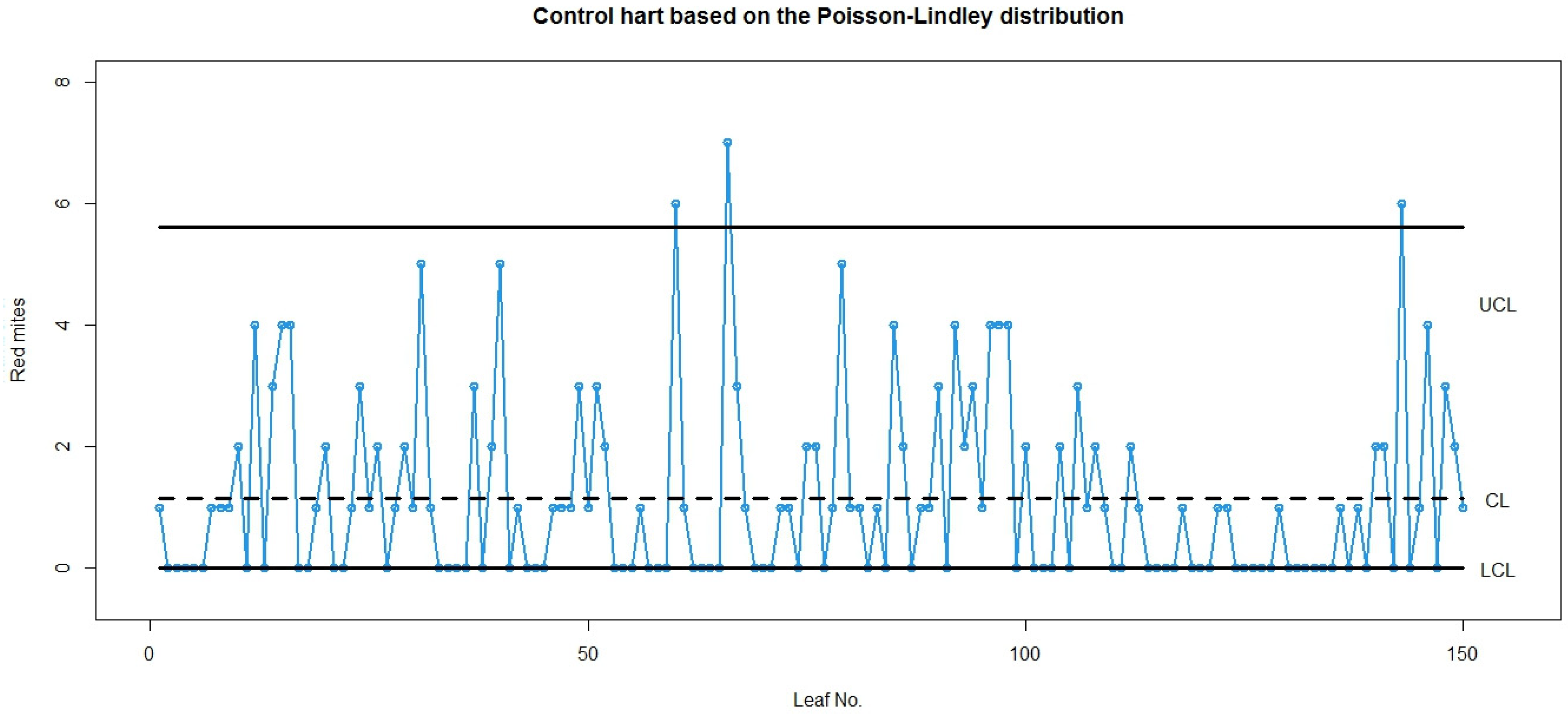
4.2. A Real Data Set Example

To assess the implementation of the control charts introduced in Section 3 on a real dataset, we considered the “number of European red mites on apple leaves” dataset available in [28]. We fitted the Poisson and Poisson–Lindley distributions to this dataset using the “fitdistrplus” package in R software.

Table 2. Goodness-of-fit statistics of Poisson and Poisson–Lindley distributions to the number of European red mites on apple leaves dataset.

Number of European Red Mites per Leaf	Observed Frequency	Expected Frequency
		Poisson Distribution	Poisson–Lindley Distribution
0	70	47.6	67.2
1	38	54.6	38.9
2	17	31.3	21.2
3	10	11.9	11.1
4	9	3.4	5.7
5	3	0.8	2.8
6	2	0.2	1.4
7	1	0.1	0.9
8	0	0.1	0.8
Total	150	150	150
ML Estimate		$\widehat{\theta }=1.146667$	$\widehat{\theta }=1.26016$
Standard Error		0.08743245	0.1139965
Chi-square Statistic		49.15817	1.251797
Chi-square d.f		3	3
Chi-square p-value		1.207139 × 10−10	0.7406099
$AIC$		487.6199	447.0218
$BIC$		490.6305	450.0324

displays the observed and expected frequencies resulting from fitting the distributions, along with estimates of the distribution parameters and goodness-of-fit statistics.

As shown in Table 2, we estimated the value of parameter $\theta$ for the Poisson distribution to be 1.146667 using the maximum likelihood $\left(ML\right)$ method. Additionally, the chi-square test statistic for fitting the Poisson distribution to the dataset is 49.15817 with a p-value nearly equal to zero (up to 9 decimal places), indicating that the assumption that the data follows the Poisson distribution is rejected. For the Poisson–Lindley distribution, we estimated parameter $\theta$ using the $ML$ method to be 1.1664. The chi-square test statistic for this distribution is 1.251797 with a p-value of 0.7406099, indicating that the $PLD$ fits the dataset well. Additionally, both the Akaike Information Criterion $\left(AIC\right)$ and Bayesian Information Criterion $\left(BIC\right)$ values for the $PLD$ are lower than the corresponding values for the Poisson distribution, demonstrating the superiority of the $PLD$ over the Poisson distribution.

We considered both an ordinary control C-chart based on the Poisson distribution and a $PLD$-based control chart for comparison in analyzing this dataset. For the C-chart, we have $CL=1.146667$, $UCL=4.359143$ (found by adding 3 times the square root of 1.146667 to the center line), and $LCL=0$ (since it is less than zero, which is not relevant for this chart). For the $PLD$-based control chart, we placed $\widehat{\theta }=1.26016$ in Equation (8) and found $CL=1.146667$, $UCL=5.604811$, and $LCL=0$ (since it is less than zero, which is not relevant for this chart).

Figure 5 and Figure 6 show the C-chart and the $PLD$-based control chart for the mentioned data sets, respectively.

Figure 5 illustrates that if one uses the C-chart without considering the fitness of the Poisson distribution to the dataset, one will incorrectly identify six out-of-control samples. Conversely, considering the results of the goodness-of-fit tests, $PLD$ should be used for these data. Figure 6 indicates that in this case, there are only three out-of-control samples.

5. Discussion and Conclusions

Statistical Process Control (SPC) commonly employs control charts as graphical and statistical tools to detect whether a process is under control. Shewhart control charts with 3-sigma control limits are widely used for monitoring industrial processes. One of the most important control charts for monitoring the number of nonconformities in production processes is the C-chart, which uses the Poisson distribution as a quality characteristic distribution. However, when the dataset is over-dispersed, the Poisson distribution may not be suitable, and the Poisson–Lindley distribution can serve as a suitable alternative.

Until now, no control chart has been designed for over-dispersed data. In this article, we reviewed some important features of the Poisson–Lindley distribution and introduced parametric control charts for both individual observations and subgroups of known and unknown parameter states. Additionally, we presented non-parametric bootstrap charts to monitor the mean and standard deviation of the Poisson–Lindley process as an algorithm. We demonstrated how to implement parametric and bootstrap control charts using a simulated example of randomly generated subgroups from the Poisson–Lindley distribution, as well as a real-world dataset. Furthermore, we evaluated the performance of bootstrap control charts using $ARL$ and $SDARL$ criteria. The results show excellent performance of the parametric and very good performance of the bootstrap control charts introduced in this paper.

References

1. Ramos, M.; Ascencio, J.; Hinojosa, M.V.; Vera, F.; Ruiz, O.; Jimenez-Feijoó, M.I.; Galindo, P. Multivariate statistical process control methods for batch production: A review focused on applications. Prod. Manuf. Res. 2021, 9, 33–55. [Google Scholar] [CrossRef]
2. Apsemidis, A.; Psarakis, S.; Moguerza, J.M. A review of machine learning kernel methods in statistical process monitoring. Comput. Ind. Eng. 2020, 142, 106376. [Google Scholar] [CrossRef]
3. Zhang, C.; Niu, S. Adaptive industrial control data analysis based on deep learning. Evol. Intell. 2023, 20, 1–9. [Google Scholar] [CrossRef]
4. Vellaisamy, P.; Upadhye, N.; Cekanavicius, V. On negative binomial approximation. Theory Probab. Its Appl. 2013, 57, 97–109. [Google Scholar] [CrossRef]
5. Sengar, A.S.; Upadhye, N.S. Subordinated compound Poisson processes of order k. Mod. Stoch. Theory Appl. 2020, 7, 395–413. [Google Scholar] [CrossRef]
6. Kumar, A.N.; Upadhye, N.S. On discrete Gibbs measure approximation to runs. Commun. Stat.-Theory Methods 2022, 51, 1488–1513. [Google Scholar] [CrossRef]
7. Sankaran, M. 275. note: The discrete poisson-lindley distribution. Biometrics 1970, 26, 145–149. [Google Scholar] [CrossRef]
8. Lindley, D.V. Fiducial distributions and Bayes’ theorem. J. R. Stat. Soc. Ser. B 1958, 20, 102–107. [Google Scholar] [CrossRef]
9. Mahmoudi, E.; Zakerzadeh, H. Generalized poisson–lindley distribution. Commun. Stat.-Theory Methods 2010, 39, 1785–1798. [Google Scholar] [CrossRef]
10. Shanker, R.; Mishra, A. A two-parameter Poisson-Lindley distribution. Int. J. Stat. Syst. 2014, 9, 79–85. [Google Scholar]
11. Hassan, A.S.; Assar, S.M.; Ali, K.A. The complementary Poisson-Lindley class of distributions. Int. J. Adv. Stat. Probab. 2015, 3, 146–160. [Google Scholar] [CrossRef]
12. Zamani, H.; Faroughi, P.; Ismail, N. Bivariate Poisson-Lindley distribution with application. J. Math. Stat. 2015, 11, 1. [Google Scholar] [CrossRef]
13. Shanker, R.; Mishra, A. On size-biased two parameter Poisson-Lindley distribution and its applications. Am. J. Math. Stat. 2017, 7, 99–107. [Google Scholar]
14. Das, K.K.; Ahmed, I.; Bhattacharjee, S. A new three-parameter Poisson-Lindley distribution for modelling over-dispersed count data. Int. J. Appl. Eng. Res. 2018, 13, 16468–16477. [Google Scholar]
15. Ghitany, M.; Al-Mutairi, D. Estimation methods for the discrete Poisson–Lindley distribution. J. Stat. Comput. Simul. 2009, 79, 1–9. [Google Scholar] [CrossRef]
16. Montgomery, D.C. Introduction to Statistical Quality Control; John Wiley & Sons: Hoboken, NJ, USA, 2020. [Google Scholar]
17. Efron, B.; Tibshirani, R.J. An Introduction to the Bootstrap; CRC Press: Boca Raton, FL, USA, 1994. [Google Scholar]
18. Bai, D.; Choi, I. X and R control charts for skewed populations. J. Qual. Technol. 1995, 27, 120–131. [Google Scholar] [CrossRef]
19. Nichols, M.D.; Padgett, W. A bootstrap control chart for Weibull percentiles. Qual. Reliab. Eng. Int. 2006, 22, 141–151. [Google Scholar] [CrossRef]
20. Lio, Y.; Park, C. A bootstrap control chart for inverse Gaussian percentiles. J. Stat. Comput. Simul. 2010, 80, 287–299. [Google Scholar] [CrossRef]
21. Lio, Y.L.; Park, C. A bootstrap control chart for Birnbaum–Saunders percentiles. Qual. Reliab. Eng. Int. 2008, 24, 585–600. [Google Scholar] [CrossRef]
22. Chiang, J.-Y.; Lio, Y.; Ng, H.; Tsai, T.-R.; Li, T. Robust bootstrap control charts for percentiles based on model selection approaches. Comput. Ind. Eng. 2018, 123, 119–133. [Google Scholar] [CrossRef]
23. Saeed, N.; Kamal, S.; Aslam, M. Percentile bootstrap control chart for monitoring process variability under non-normal processes. Sci. Iran. 2021, in press. [CrossRef]
24. Ma, Z.; Park, C.; Wang, M. A Robust Bootstrap Control Chart for the Log-Logistic Percentiles. J. Stat. Theory Pract. 2022, 16, 3. [Google Scholar] [CrossRef]
25. Seppala, T.; Moskowitz, H.; Plante, R.; Tang, J. Statistical process control via the subgroup bootstrap. J. Qual. Technol. 1995, 27, 139–153. [Google Scholar] [CrossRef]
26. Liu, R.Y.; Tang, J. Control charts for dependent and independent measurements based on bootstrap methods. J. Am. Stat. Assoc. 1996, 91, 1694–1700. [Google Scholar] [CrossRef]
27. Jones, L.A.; Woodall, W.H. The performance of bootstrap control charts. J. Qual. Technol. 1998, 30, 362–375. [Google Scholar] [CrossRef]
28. Bliss, C.I.; Fisher, R.A. Fitting the negative binomial distribution to biological data. Biometrics 1953, 9, 176–200. [Google Scholar] [CrossRef]
Figure 1. The Poisson–Lindley distribution’s pmf at different θ values: (a) 0.25, (b) 0.5, (c) 1, and (d) 2.
Mathematics 11 02428 g001
Figure 2. Control chart for randomly generated subgroups of size 5 from the P L D .
Mathematics 11 02428 g002
Figure 3. Bootstrap control M-chart for randomly generated subgroups of size 5 from the P L D .
Mathematics 11 02428 g003
Figure 4. Bootstrap control S-chart for randomly generated subgroups of size 5 from the P L D .
Mathematics 11 02428 g004
Figure 5. C-chart for the number of European red mites on apple leaves data set.
Mathematics 11 02428 g005
Figure 6. The P L D based control chart for the number of European red mites on apple leaves data set.
Mathematics 11 02428 g006