Kit of Uniformly Deployed Sets for p-Location Problems

Abstract

This paper deals with p-location problem solving processes based on a decomposition, which separates the creation of a uniformly deployed set of p-location problems from the solution of the p-location problem for that specific instance. The research presented in this paper is focused on methods of construction of uniformly deployed sets of solutions and the examination of their impact on the efficiency of subsequent optimization algorithms. The approaches to the construction are used for the constitution of predetermined families of uniformly deployed sets of p-location problem solutions, which have standard sizes. We introduce two methods of uniformly deployed set construction: the first one is based on composition, followed by an enlargement process; and the second one makes use of voltage graphs. The construction approaches are completed by an algorithm, which adjusts the set of solutions to the sizes of a solved instance. The influence of a set construction approach on solving process efficiency is studied on real-world benchmarks, which include both the p-median objective function and the generalized disutility function. The solving process is performed alternatively using the swap or path-relinking based methods. Results of the computational study obtained by all combinations of the mentioned approaches are presented and evaluated in the concluding part of the paper to make the studied characteristics visible.

1. Introduction

The term “p-location problem” is used within this paper to denote a large family of location problems, which correspond to tasks of deploying a determined number of facilities in a given finite set of feasible places so that the objective function of the facility deployment takes the minimal or maximal value. The class of p-location problems includes well-known p-median problems as well as non-standard problems arising from their generalization. As far as the classical formulation is concerned, work [1] introduces discrete network location models with definitions of p-median and p-center, etc. Definitions of weighted versions of these problems can be found in [2]. Related problems concerning dispersion of p facilities are referred to in [3,4,5]. Work [6] is a survey on location models in the public sector, which comprises the deployment of fire brigades or police stations and the design of the medical emergency service system.

A survey of ambulance location models with definitions of the most important problems can be found in [7]. Papers [8,9] study ambulance location problems represented as a generalization of the covering problem. The references [10,11] contain the studies of modified versions of ambulance location and relocation problems. In papers [12,13,14], various versions of the p-median problem are studied.

All the listed variants of the problem have one common property: their solution can be described by a binary m-dimensional vector containing exactly p unit components.

The original p-median and weighted p-median problems are easy to model by means of linear integer programming with classical allocation constraints, and solve via a standard integer programming method [4,15]. Nevertheless, this approach proved to be ineffective when bigger instances of the problems have to be solved. This inefficiency was mitigated to some extent by developing so called radius formulation of the problems [16,17,18,19]. Despite much progress in developing exact methods, the unpredictable computational time of the branch-and-bound method focuses researchers’ attention on various kinds of evolutionary metaheuristics.

Genetic algorithms were studied in [20,21]. A scatter search algorithm was reported in [22].

This research is motivated by recent findings [23] that even a simple heuristic can reach a near-to-optimal solution. Due to the special feature of the set of all feasible solutions of the p-location problem, a special heuristic can be used to exclude inadmissible solutions from the starting uniformly deployed set. These are replaced by a smaller set of better solutions, continuing to the point when the most recent set contains only the best pair of found solutions. The starting set of solutions was obtained by a manually created subset of solutions and their step-by step augmentation using integer programming tools. Another approach to the starting set creation was proposed in [24], where a new approach based on graph theory was used.

It was found that the efficiency of the heuristics depends on preliminary information about the objective function course on the set of feasible solutions. Such a finding may help in the determination of promising initial solutions for a searching process based on the neighborhood search, or it can provide metaheuristics imitating evolutionary processes or social behavior of species with a set of initial problem solutions. For example, genetic algorithms [20,21] start with a population of problem solutions, which should differ as much as possible. A scatter search algorithm [22] maintains two parts of a reference set of solutions, where the first part contains a collection of good solutions and the other one represents a maximally diversified set of solutions. In addition, a swarm particle optimization algorithm [23,25] needs a set of good initial positions for the swarm particles. This paper focuses on a way to create a diverse set of solutions. Diversification of the set of problem solutions is a substantial part of all of the above-mentioned metaheuristics. The phase of diversification prevents the searching processes from reaching a so called homogeneous population, which is equivalent to being trapped at a local minimum.

Information about objective function values of the p-location problem can be obtained by sampling the objective function at solutions of a small subset of all feasible solutions.

To obtain relevant information, we try to cover the set of all feasible solutions with a limited number of samples, so that a distance between any pair of solutions is greater than a given constant. Such a set of solutions is called uniformly deployed over the set of all solutions. One way to achieve an admissible uniformly deployed set is to use the iterative process. Thus, a step-by step process maximizes the subset cardinality, subject to the condition that the mutual distance between any pair of solutions exceeds a given limit.

A standard approach to creating a uniformly deployed set (UDS) for a given number of possible facility locations and a given number of facilities entails creating a basic set and the subsequent step-by-step augmentation of this set by ongoing solutions.

This way of creating a UDS is very expensive when it comes to computational time demanded, especially in the concluding augmentation steps. Usage of set construction methods in combination with a fast heuristic may erase the effect of the UDS creation on solving process efficiency [26,27,28].

Nevertheless, a standard kit of UDS for public use allows for the removal of the computational burden of UDS generation from the solving process applied to an instance of the solved problem [29]. This paper is devoted to the kit construction and its exploitation for neighborhood and path-relinking-based searches. Special attention is paid to the basic set creation in the process of individual UDS construction and to the adjustment of a kit set to the size of a given p-location problem.

2. The p-Location Problem and Uniformly Deployed Set

The p-location problem may be tackled as a challenge of deploying p facilities in a set of m suitable places so that a given objective function reaches the minimal value. These kinds of networks are usually associated with network nodes. The decision at a facility located at a place i is modelled by a binary variable y_i, which takes the value of one if a facility is located at place i, with the zero value corresponding to the opposite decision. This way, the solving process of the p-location problem can be formulated as a search in a finite domain consisting of some vertices of a unit hypercube in the m-dimensional Euclidean space, where each feasible solution corresponds to a vertex described by zero-one vector y, which has exactly p non-zero components. Thus, (1) may describe the set Y of all feasible solutions of the problem.

$$\mathit{Y}=\left\{\mathit{y}:\hspace{0.17em}\hspace{0.17em}{y}_i\in \left\{0,\hspace{0.17em}\hspace{0.17em}1\right\},\hspace{0.17em}\hspace{0.17em}{\displaystyle \sum _{i=1}^m{y}_i}\hspace{0.17em}=p\right\}$$

(1)

Here, we present the two most frequent examples of the p-location problem, which can be applied to the design of a public service system. We assume that the public service system provides services to a set of users. Their locations also correspond to network nodes, and they are denoted by integers from 1 to n. A user j = 1 … n is assigned by a weight b_j, which can stay for the frequency of the visits at the user j and d_ij denotes the network time-distance between locations i and j.

The standard weighted p-median problem formulation considers that each user demand is satisfied by the nearest located service center, and the minimized user’s disutility is expressed by the average time-distance from a user to the nearest located service center. This problem is described by (2).

$$\min \left\{F^s(\mathit{y})={\displaystyle \sum _{j=1}^n{b}_j\min \left\{d_{ij}\hspace{0.17em}:\hspace{0.17em}\hspace{0.17em}i=1,\hspace{0.17em}\dots ,\hspace{0.17em}m\hspace{0.17em};\hspace{0.17em}{y}_i=1\right\}}:\hspace{1em}\mathit{y}\in \mathit{Y}\right\}$$

(2)

However, if the service system satisfies randomly emerging demands for service, then the rule of the nearest service center cannot be followed due to possible center occupancy by an earlier request. In such a case, the system operates as a queuing system with p service lines.

The generalized problem formulation considers a set of {i₁(j), …, i_r(j)} of r nearest center locations to a user j and it is assumed that the demand of user j is satisfied from center location i_k(j) with probability q_k.

In this case, the minimized user’s disutility is expressed by the expected average time-distance from a user to the nearest available service center [30]. The associated generalized p-location problem can be briefly formulated as follows.

$$\min \left\{F^g(\mathit{y})={\displaystyle \sum _{j=1}^n{b}_j{\displaystyle \sum _{k=1}^r{q}_k{\min }_k\left\{d_{ij}\hspace{0.17em}:\hspace{0.17em}\hspace{0.17em}i=1,\hspace{0.17em}\dots ,\hspace{0.17em}m\hspace{0.17em};\hspace{0.17em}{y}_i=1\right\}:\hspace{0.17em}\hspace{0.17em}\mathit{y}\in \mathit{Y}}}\right\}$$

(3)

In the above objective function expression, the operation min_k{range} returns the k-th minimal value of the range.

Further, we devote our attention to specifics of the set Y of feasible hypercube vertices corresponding with feasible solutions of the problems (2) and (3) [27]. To study the structure of the set of the unit hypercube vertices, we use the well-known notion of Hamming distance. Hamming distance H(x, y) between two hypercube vertices described by vectors y and x is given by (4).

$$\hspace{0.17em}\hspace{0.17em}H\left(\mathit{y},\hspace{0.17em}\mathit{x}\right)=\hspace{0.17em}{\displaystyle \sum _{i=1}^m\left|y_i-x_i\right|}$$

(4)

It is obvious that the value H(x, y) is an integer, and it varies from the value of two up to the value of 2p for any pair distinct vectors. The case H(y, x) = 2 corresponds with the instance when all but two components of y and x are identical. This means that the associated solutions differ only in one service center location. The Hamming distance can be used to define various topologies on the set Y. The smallest neighborhood of a point y can be defined as a set of x∈Y, which satisfies the constraint H(y, x) = 2. This neighborhood consists of p(m − p) neighboring solutions.

It can be seen that integer value t = p − H(y, x)/2 is equal to the number of located centers contained in both solutions y and x. To obtain relevant information about the objective function on Y with minimal computational effort, we try to constitute a subset of Y, the cardinality of which is adequate for a given purpose and in which the elements of Y are uniformly deployed over the set of all solutions. In the ideal case, the subset elements must satisfy the conditions that the mutual distance between two solutions is greater than or equal to a given limit and that it is impossible to enlarge the subset by another solution under the distance condition.

The UDS of p-location problem solutions can be presented as a maximal subset S of feasible solutions of Y so that the condition H(y, x) ≥ h is fulfilled for each x, y ∈ S and for given h. For practical use, we also accept breaking the condition of maximality and replacing it with a request that the subset cardinality reaches a sufficient value. This weaker definition is applied in situations when we search for a subset, the cardinality of which exceeds a demanded size, and the condition H(y, x) ≥ h is fulfilled for the maximal possible value of h.

3. Fast Minimization Heuristics for the p-Location Problem

Within the paper, the contribution of the uniformly deployed sets to the efficiency of simple minimization heuristics is studied. Attention is paid to the neighborhood and path-relinking-based searches introduced in [31]. The swap algorithm equipped with the best admissible strategy represents the mode of neighborhood search, which consists of the solutions meeting the constraint H(y, x) = 2. In the swap algorithm described below, an individual solution given by an m-dimensional zero-one vector y is represented by a set L of center locations occupied by a center, i.e., L = {I ∈ {1, …, m}: y_i = 1}. The same representation will be used in the path-relinking search. The denotation f(L) stands for the values of F^s(y) or F^g(y) computed for vector y, which corresponds to L. The algorithm Swap comes from an initial solution L and performs according to the following steps:

Swap(L)

0.

Initialize f^** = f^* = f(L), P = {1, …, m} − L and go to 1.

1.

For each location I ∈ L do step 2 and then go to 4.

2.

For each unoccupied location g ∈ P do step 3.

3.

Put L = (L − {i}) ∪ {g}and compute f(L), if f(L) < f^*, then put f^* = f(L) and L^* = L.

4.

If f^** ≤ f^* then terminate, return solution L^* and its objective function value f^* as the output, else put f^** = f^*, L = L^*, P = {1 … m} − L and go to 1.

The original version of the path-relinking method presented by [17] proceeds along one of the shortest paths, which links a pair of input solutions. The procedure examines the solutions on the inspected paths and returns the best feasible solution on the path. Having demonstrated the performance of the original path-relinking method in an m-dimensional unit hypercube, the inspected path is presented by an alternating sequence of the hypercube vertices and edges connecting the neighboring vertices. A hypercube edge connects two vertices, which differ only in one component. Hence, the Hamming distance of these vertices is equal to one. It follows from this fact that the number of unit components of the succeeding vertices of the inspected path cannot equal p and hence at least every second vertex of the path does not belong to the set Y.

To skip the examination of the idle vertices, we proposed a special version of the path-relinking method for the p-location problems, which inspects only feasible solutions on the shortest paths [31].

To achieve this effect, we replaced the original inversion operation with a swap operation, where the neighbor of the current solution lying on the shortest path on the surface of the hypercube is searched for. Since the swap operation preserves the number of occupied locations, each inspected solution has exactly p occupied locations.

In the suggested form of the path-relinking approach, two lists L₁ and L₂ are used. The lists of the p service center locations correspond with the two input solutions. In the next method description, the lists will be handled as ordinary sets. To describe the method in a concise way, we introduce auxiliary sets P₁ ⊆ L₁ and P₂ ⊆ L₂ defined by P₁ = L₁ − L₂ and P₂ = L₂ − L₁. The algorithm Path-RelinkingMethod(L₁, L₂) is described below, and the algorithm returns the resulting solution L^*, which is the best-found solution met on the inspected path.

Path-RelinkingMethod(L₁, L₂)

0.

Initialize the best-found solution L^* and the auxiliary sets P₁ and P₂ by L^* = argmin{f(L₁), f(L₂)}, P₁ = L₁ − L₂ and P₂ = L₂ − L₁.

1.

Find locations i^* ∈ P₁ and j^* ∈ P₂ to minimize the function f((P − {i}) ∪ {j}) and update L₁, P₁, P₂ and L^* according to L₁ = (L₁ − {i^*}) ∪ {j^*}, P₁ = P₁ − {i^*}, P₂ = P₂ − {j^*} and L^* = argmin{f(L^*), f(L₁)},

2.

If | P₁ | = | P₂ | = 1, then stop the process and return L^*, else exchange L₁ with L₂, P₁ with P₂, and go to 1.

Both methods inspect a neighborhood of a current solution denoted by either L or L₁. The neighborhood is determined by all p-location problem solutions, which can be obtained by one exchange of a location included in the solution with a location, which belongs to P or P₂, respectively. The time necessary for one neighborhood inspection depends mostly on the time needed for the computation of objective function (2) or (3) of a solution of the neighborhood. The fact that the solution from the neighborhood differs only in one location can be used for a considerable complexity reduction. While computing the functions F^s and F^g in accordance with (2) or (3) has the complexity O(np) or O(npr), the used implementation reduces the computational complexity to O(n) or O(nr), respectively.

4. Kit of Uniformly Deployed Sets

The computation of satisfactorily large UDS for an individual problem characterized by the number m of possible center locations and by the number p of located centers turned out to be quite time-demanding [27]. To avoid the load of solving process, we proposed the concept of a UDS kit, which allows the separation of the activities associated with generating a uniformly distributed set from the solving of the p-location problem.

The principle of a UDS kit is based on a separation of the computational effort connected with the p-location problem solution into two parts. The first one accounts for the creation of a general structure—a UDS. The second part represents the solving process. Even if a UDS of the p-location problem solutions depends only on two parameters p and m of the problem instance, the number of possible combinations of the parameter values is too large to create a corresponding UDS for each of these combinations in advance. That is why a finite range M of numbers m is determined. Furthermore, a finite range P_m for each m ∈ M is designed (in this paper we state M = {75, 100, 200, …, 1000} and P_m = {10, 20, …, m/3}) and then a kit of uniformly deployed sets is established so that a uniformly deployed set S_mp is created for each m ∈ M and p ∈ P_m. For practical reasons, the S_mp creation is subject to a demand for a minimal number of elements. Such a kit may be created independently of its further exploitation.

If there is a need to solve a p-location problem instance with parameters m and p, which do not belong to the ranges M and P_m, then a tight approximation m ∈ M and p ∈ P_m of the parameters must be found so that m ≤ m and p ≤ p. The corresponding member S_mp of the kit must be adjusted to fit the number p of locations, which determines a feasible solution for the problem instance. The adjustment can be simply performed by removing the p − p last elements of each p-tuple contained in S_mp. After the adjustment, the minimal Hamming distance of a pair of p-location problem solutions is 2(p − t), where t denotes the minimal number of common locations contained in each solution of the pair.

It was proved that this reduction does not affect the efficiency of the algorithms based on the neighborhood search, but it may considerably spoil the resulting quality of the used path-relinking-based algorithm.

This defect can be explained by the fact that no solution of the reduced set S_mp after the reduction contains any of the m − m locations, which were missing in solutions of the original kit member S_mp. As the path-relinking method examines the shortest path between the input vertices of a unit m-dimensional hypercube, it is unable to leave the m-dimensional sub-space and explore any solution outside the sub-space.

To remove this defect of kit usage, we propose an extension method, which incorporates the surplus possible service center locations into solutions of the chosen kit set. The following extension algorithm assumes that the solutions of the set S are represented by zero-one m-dimensional vectors y^k for k= 1, …, |S|, where the last m-m components are equal to zero. In the algorithm below, the symbols Y_i and Q are defined by (5) and (6), respectively.

Extension(S, m, m)

0.

Compute Y_i for i = 1 … m according to (5); compute Q according to (6) and define Q‘ = min{m-m, Q}; initialize t = m.

1.

For each k = 1 … |S| perform the following cycle

for each I = 1 … m perform the following command

if (y_i^k = 1) and (Y_i > 1) and (t < m + Q’) then do

y_i^k = 0; y_t^k = 1; Y_i = Y_i − 1; t = t + 1.

$$Y_i={\displaystyle \sum _{k=1}^{\left|S\right|}{y}_i^k}$$

(5)

$$Q={\displaystyle \sum _{i=1}^{\underset{\_}{m}}\max \left\{0,Y_i\right\}}$$

(6)

The above extension algorithm inserts Q’ unused locations into elements of the input uniformly deployed set, unless diminishing the Hamming distance among the solutions.

After having adjusted the kit set to the size of the solved p-location problem, the Swap and the Path-relinking algorithms can exploit the UDS in the following ways. Let an adjusted uniformly deployed set S be given, and then the following steps are performed.

(a)

Compute f(L) for each L∈S and initialize L^* by the solution with the lowest value of the objective function.

(b)

Run the algorithm Swap(L^*).

An adjusted uniformly deployed set S can be used as an initial swarm in searching strategies using the path-relinking-based inspection as a tool for the best-found-solution improvement. Let the expression Path-RelinkingMethod(L₁, L₂) denote the resulting solution returned by the path-relinking method applied to input solutions L₁ and L₂. Let the set S consists of solutions L₁, L₂, …, L_|S| ordered by a permutation U in a sequence, which satisfies f(L_U(1)) ≤ f(L_U(2)) ≤ …≤ f(L_U(|S|)). Then, a search based on the path-relinking method can be suggested as follows.

0.

Initialize L^* by solution L_U(1).

1.

Perform command L^* = Path-RelinkingMethod(L^*, L_U(k)) repeatedly for k = 2 … |S|.

2.

Return the resulting solution L^*.

5. Composition Approach to Uniformly Deployed Set Construction

For given integers m ∈ M and p ∈ P_m, the corresponding uniformly deployed set S_mp is constructed according to the following process.

First, an attempt at maximal uniformly deployed set S¹_q construction was performed for the q-location problem defined for q² possible center locations for any integer q from the range {2, 3, …, 31} so that arbitrary two q-tuples contain at most one conjoint element, i.e., t = 1. Second, a basic UDS for given m∈M and p∈P_m was composed of k q-tuples of S¹_q and of k(p − q) other locations, where k and q were determined so that k(p − q) + q² ≤ m holds. Each pair of p-tuples of the basic set have at most one common location.

The resulting basic set can be submitted to the time-restricted process augmentation, which solves the linear programming problem described by the models (7)–(11) in each step of the augmentation. The initial value of parameter t equals one. If the cardinality of the augmented set did not reach a given threshold, the parameter t is incremented, and the augmentation process continues. This augmentation process can be applied to an arbitrary basic uniformly deployed set regardless of its value of t.

Let the basic set of p-location problem solutions satisfy the property that no pair of solutions may contain more than t common locations; thus, the minimal Hamming distance of the solutions equals 2(p − t). The basic set is iteratively augmented by the problems (7)–(11). The optimal solution y of the problems (7)–(11) is added to the current set S under the condition that the value (7) of the optimal solution equals zero. This augmenting process stops either if the optimal value of (7) is positive or the given cardinality of the set S is achieved or the computational time limit is exceeded. The model was originally published in [27].

Let s be an element of the set S. The solution s is represented by a set of p center locations. The solution can be described by m-dimensional zero-one vector e_s, where the i-th component e_si equals one if the location i is an element of the set s. Otherwise, the component e_si takes the value of zero. Let us use a series of binary variables y_i ∈ {0, 1} for i = 1 … m to describe an additional solution y, that could extend the current set S. Furthermore, we use an additional series of variables z, where variable z_s is associated with the solution s and gives the number of common locations of the solution s and y reduced by the value of t.

$$Minimize{\displaystyle \sum _{s\in S}{z}_s}$$

(7)

$$Subject\hspace{0.17em}\hspace{0.17em}to{\displaystyle \sum _{i=1}^m{y}_i}=p$$

(8)

$${\displaystyle \sum _{i=1}^m{e}_{si}{y}_i}\le t+z_s\hspace{0.17em}\hspace{0.17em}\hspace{0.17em}\hspace{0.17em}\hspace{0.17em}for\hspace{0.17em}\hspace{0.17em}s\in S$$

(9)

$$y_i\in \left\{0,\hspace{0.17em}1\right\}\hspace{0.17em}\hspace{0.17em}\hspace{0.17em}\hspace{0.17em}\hspace{0.17em}for\hspace{0.17em}\hspace{0.17em}i=1,\hspace{0.17em}\hspace{0.17em}\dots ,\hspace{0.17em}\hspace{0.17em}m$$

(10)

$$z_s\ge \hspace{0.17em}0\hspace{0.17em}\hspace{0.17em}\hspace{0.17em}\hspace{0.17em}for\hspace{0.17em}s\in S$$

(11)

The expression (7) stands for the total of surpluses above the value t of conjoint locations of the solution modelled by y and the input solution s ∈ S. In the case when the expression (7) takes the value of zero, then an arbitrary solution from S and the solution modelled by y have at most t common locations. Constraint (8) assures the feasibility of the solution described by the vector y. Constraint (9) ensures connections between the solution y and the additional variables z_s for s∈ S. The left part of (9) for a solution s expresses the number of locations common for solutions s and y. If the value exceeds t, the associated variable z_s must get a value greater than or equal to the surplus.

6. Graph-Based Approach to Uniformly Deployed Set Construction

In this section, we present the construction of uniformly deployed sets from a special class of digraphs called monopoles. The advantage of this approach is that UDS with given parameters can be computed directly. The origins of this method trace back to the topological graph theory [32] and it serves for the construction of large graphs and digraphs with given properties.

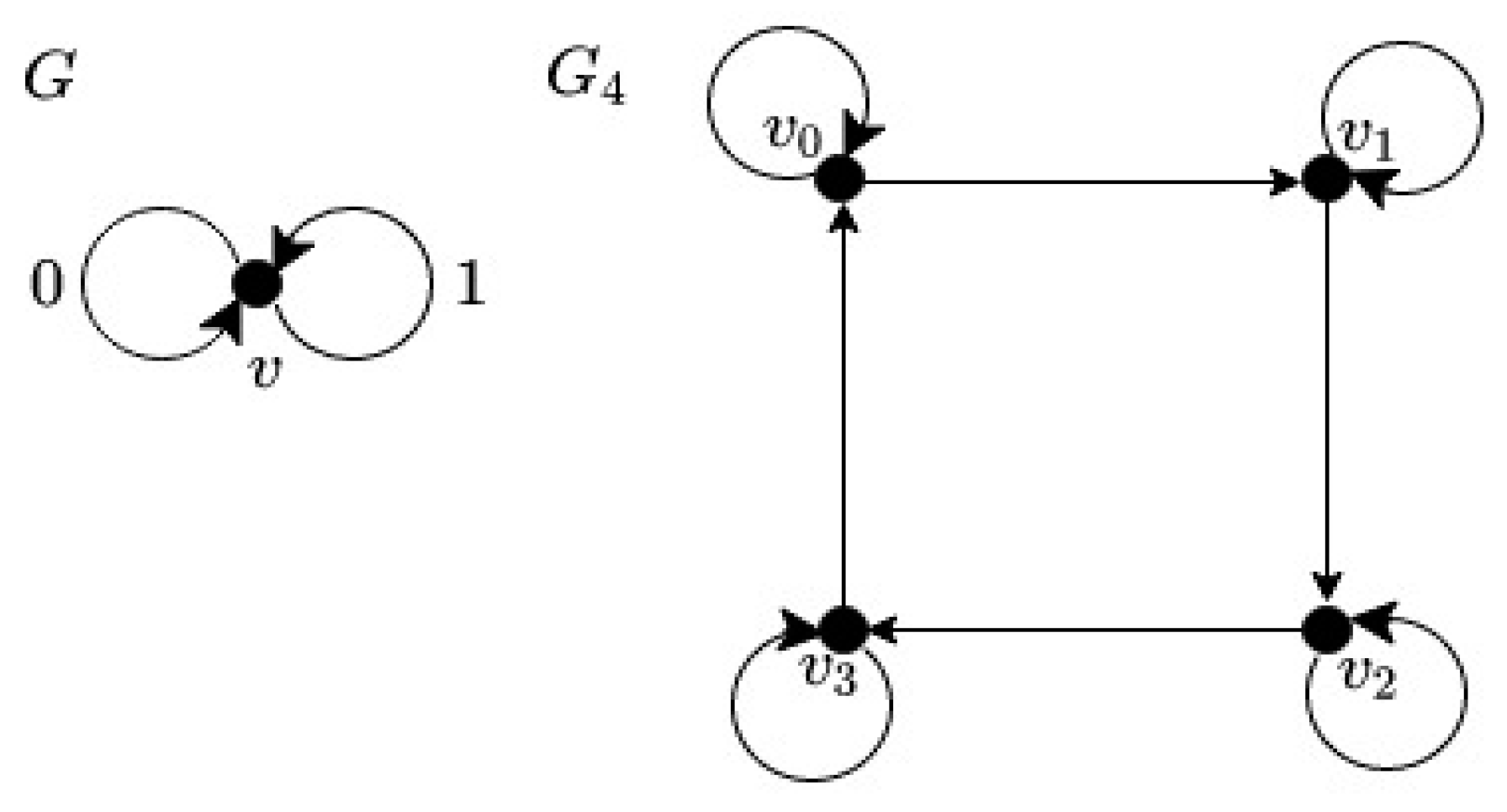
For our purposes, we use the smallest possible digraph - monopole, which contains only one vertex v and p edges e₁, e₂, …, e_p. Each edge has an assigned value a(e_i) = a_i, which is called the voltage of the edge. In origin, the voltages are elements of an appropriate (usually abelian) group. However, we consider the elements of the set Z_m = {0, 1, …, m − 1}. Such a digraph is called a voltage digraph G = (V, E, a), where V = {v} is the vertex set, E = {e₁, e₂, …, e_p} is the set of edges and a:E→Z_m is an assignment of voltages. From G and Z_m, we can create a derived digraph G_m = (V_m, E_m), where V_m = {v₀, v₁, …, v_m−1} and the edge (v_i, v_j) belongs to the set E_m if and only if, there is an edge e in E, and voltage a from Z_m such that mod(i + a,m) = j (where mod(x,m) represents the remainder after dividing x by m). An example of the construction for G₄ and Z₄ is depicted in Figure 1.

In the paper [33], we introduced a construction of the Hoffmann–Singleton graph from the voltage graph. It follows from the properties of the Hoffmann–Singleton graph (each pair of neighboring vertices has no conjoint neighbor, and each pair of non-adjacent vertices has exactly one conjoint neighbor) that the rows of its adjacency matrix form the uniformly deployed set with parameters m = 50, p = 7, and t = 1. It is known that these graphs (strongly regular graphs with some special parameters) occur rarely. However, if we use weaker conditions for such objects, then we can construct derived digraphs with appropriate properties. These conditions can be stated as follows:

0.

The derived digraph has m vertices.

1.

Each vertex has out-degree p.

2.

Each pair of vertices has at most t common successors.

Condition 1 ensures that the adjacency matrix of the derived digraph has m rows (elements of UDS) and m columns (candidates for service centers location). Condition 2 ensures that each row of the adjacency matrix contains exactly p ones. Condition 3 ensures that each pair of rows has at most t ones on the same position. If the voltage graph is monopole with p loops and we use the set Z_m, then conditions 1 and 2 are fulfilled. The choice of appropriate voltages can ensure that each pair of vertices in G_m has at most t common successors. We introduce a simple and fast procedure that computes such p element subset of Z_m. It is possible to show that for all v_i, v_j ∈ V_m a pair (v_i, v_x) is the edge in G_m if and only if a pair (v_j, v_y) is the edge in G_m (where x = mod(i + k, m) and y = mod(j + k, m)). Hence, it is enough to consider common successors of the vertices v₀, v_j. Let us suppose that v₀ and v_j have t common successors - say v_k1, v_k2, …, v_kt. Then, there are voltages k₁, k₂, …, k_t and s₁, s₂, …, s_t on loops of G such that all equations in (12) hold.

$$k_1=mod\left(j+s_1,m\right),k_2=mod\left(j+s_2,m\right),\hspace{0.17em}\dots ,k_t=mod\left(j+s_t,m\right)$$

(12)

From Equations (12) we have the expression (13).

$$j=mod\left(k_1-s_1,m\right)=mod\left(k_2-s_2,m\right)=\dots =mod\left(k_t-s_t,m\right)$$

(13)

The number of common successors of vertices v₀ and v_j is given by the number of computations mod(k − s, m) with voltages that have result j. If k, s < m/2, then mod(k − s, m) < m/2 for k > s, and mod(k − s, m) > m/2 for s > k. If we choose all voltages less than m/2, then it is enough to check the repetition of values k-s for k > s. This can be done in t-sequences: a t-sequence is an increasing sequence ${\left\{a_i\right\}}_{i=0}^q$ such that

• a₀ = 0, a₁ = 1.
• For k > 2, a_k is the minimum value such that for i ∈ {1, …, k − 1}, the value a_k − a_i occurs between values a_j − a_i (where1 ≤ i < j < k) at most t − 1 times.

From the definition of a t-sequence, we also obtain a simple algorithm for the computation of its values. Examples of the first q = 15 members of t-sequences for t = 1, 2, 3, 4 can be seen below:

t = 1 0, 1, 3, 7, 12, 20, 30, 44, 65, 80, 96, 122, 147, 181, 203

t = 2 0, 1, 2, 4, 7, 11, 16, 22, 30, 38, 48, 61, 73, 86, 103

t = 3 0, 1, 2, 3, 5, 8, 12, 16, 21, 27, 33, 40, 48, 57, 71

t = 4 0, 1, 2, 3, 4, 6, 9, 13,17, 22, 27, 33, 39, 46, 53

If we want to construct a derived digraph G_m, then we need to find such a t-sequence in which a_p−1 < m/2. The values a₀, a₁, …, a_p−1 are voltages on loops and the rows of the adjacency matrix of G_m form a uniformly deployed set for parameters m, p. More information about the construction of uniformly deployed sets can be found in [24].

7. Computational Study

Further experiments were aimed at exploration of the impact of the way in which the kit sets are suggested on the efficiency of the above-described fast minimization heuristics.

The instances used in experiments represent eight self-governing regions of the Slovak Republic. Since these regions are characterized by high geographical variability, these benchmarks are convenient for this type of testing. In the Bratislava and Trnava regions, plains and industry dominate. The Nitra region is typical agricultural flatland. The Košice region represents a mix of industry and agriculture. The Trenčín region is characterized by hills and industry. Žilina and Banská Bystrica are regions covered by mountains with several industrial centers. The Prešov region is a typical rural region covered by mountains. Each region is characterized by a set of dwelling places and the population of the associated community. The dwelling places correspond to nodes of the regional road network, which was used to compute network distances for each pair of nodes. A current medical emergency system was used to derive the number of service centers, which can be located at the set of road network nodes. Each node was considered as a possible service center location and each node-dwelling place j with population b_j was taken as a possible system user, in which volume of demands is proportional to the size of the population. In the remainder of the paper, the regions are denoted by abbreviations of the names of regional capitals. We use BA for Bratislava, BB for Banska Bystrica, KE for Košice, NR for Nitra, PO for Prešov, TN for Trenčín, TT for Trnava, and ZA for Žilina. The number m of possible center locations and the number p of centers that need to be located are plotted in

Table 1. Benchmark descriptions.

Region	m	p	m	p	Optimal Solution
					Fs	Fg
BA	87	14	75	20	19,325	26,650
BB	515	36	500	40	29,873	44,752
KE	460	32	400	40	31,200	45,588
NR	350	27	300	30	34,041	48,940
PO	664	32	600	40	39,073	56,704
TN	276	21	200	30	25,099	35,275
TT	249	18	200	20	28,206	41,338
ZA	315	29	300	30	28,967	42,110

for the individual regions. The coefficients b_j used in the objective functions of the mathematical models (2) and (3) were determined as the sizes of the dwelling place population given in hundreds of inhabitants. If the generalized problem Formulation (3) is considered, then the number r of the nearest service centers taken into account was set at the value of three. The coefficients q_k were given in percentage: q₁ = 77.063, q₂ = 16.476, and q₃ = 100 − q₁ − q₂. These parameter settings come from simulation experiments with the emergency service system of the Slovak Republic [34]. The benchmark sizes are reported in Table 1 together with objective function values F^s and F^g of optimal solutions for both formulations (2) and (3) according to [26,28]. The used kit was established for domains M = {75, 100, 200, …, 1000} and P_m = {10, 20, …, m/3}; the corresponding sizes m and p of the uniformly deployed sets withdrawn from the kit are also reported in Table 1.

To verify the hypothesis concerning the fast heuristics described in Section 3, we implemented them in the programming language JAVA, each in two versions. Versions denoted by “Swap” and “Path-relinking” solve problems described by (2) and “SwapG” and “Path-relinkingG” were designed for solving problems described by (3).

We used two series of uniformly deployed sets for the experiments. The first series was derived by reduction of the kit sets obtained by the process described in Section 5 and it is reported as “kit standard” in the remainder of the paper. The standard kit sets for the above-mentioned ranges were created for the threshold of 90 p-tuples, where the computational time was restricted to ten minutes. The final values of parameter t, for which the limit was reached, correspond also to the maximal number of common locations in two p-tuples. The values of t and uniformly deployed set cardinalities |S| are reported in

Table 2. Characteristics of the derived kit sets.

Region	m	p	“Kit Standard”				“Kit Graph”
			|S|	m	p	t	|S|	m	p	t
BA	87	14	158	75	20	7	75	75	20	13
BB	515	36	206	500	40	4	500	500	40	9
KE	460	32	200	400	40	5	400	400	40	14
NR	350	27	202	300	30	4	300	300	30	8
PO	664	32	147	600	40	3	600	600	40	7
TN	276	21	217	200	30	6	200	200	30	14
TT	249	18	205	200	20	3	200	200	20	11
ZA	315	29	202	300	30	4	300	300	30	8

. The second series denoted by the title “kit graph” was obtained from the graph-based approach described in Section 6.

To make the following comparison of the kit construction more robust, we generated ten different starting sets of solutions by random permutation of m original locations of the input uniformly deployed set, making use of the proposition that arbitrary permutation does not change parameters of the obtained set. This way, we obtained two series of ten starting sets, one for the original set denoted “kit standard” and the other for the original set called “kit graph”.

The tested approaches were applied to both problems (2) and (3) with each starting set from both series “kit standard” and “kit graph”.

Each uniformly deployed set coming from a kit was submitted to the extension described in Section 4. The results of the experiments are reported in

Table 3. Average results of the weighted p-median problem-solving process for starting series “kit standard”.

Benchmark	OptObj	“Swap“				“Path-Relinking”
		F*min	F*avg	gap	T [s]	F*min	F*avg	gap	T [s]
BA	19,325	19,325	19,325.0	0.00	0.01	19,325	19,589.2	1.37	0.04
BB	29,873	29,873	29,894.6	0.07	0.89	29,873	30,066.4	0.65	4.49
KE	31,200	31,200	31,240.7	0.13	0.56	31,200	31,319.4	0.38	2.58
NR	34,041	34,041	34,132.3	0.27	0.24	34,041	34,143.9	0.30	1.25
PO	39,073	39,073	39,106.6	0.09	1.22	39,080	39,304.7	0.59	3.15
TN	25,099	25,099	25,112.0	0.05	0.09	25,099	25,648.0	2.19	0.45
TT	28,206	28,206	28,222.6	0.06	0.06	28,206	28,226.6	0.07	0.29
ZA	28,967	28,967	28,978.8	0.04	0.22	28,967	29,004.6	0.13	1.32

,

Table 4. Average results of the weighted p-median problem-solving process for starting series “kit graph”.

Benchmark	OptObj	“Swap“				“Path-Relinking”
		F*min	F*avg	gap	T [s]	F*min	F*avg	gap	T [s]
BA	19,325	19,325	19,325.0	0.00	0.01	19,325	19,462.3	0.71	0.02
BB	29,873	29,873	29,901.2	0.09	0.87	29,873	29,875.4	0.01	10.92
KE	31,200	31,200	31,230.6	0.10	0.59	31,200	31,210.4	0.03	5.31
NR	34,041	34,041	34,077.3	0.11	0.21	34,041	34,126.5	0.25	1.86
PO	39,073	39,073	39,105.8	0.08	1.29	39,073	39,082.5	0.02	12.71
TN	25,099	25,099	25,106.8	0.03	0.09	25,099	25,110.7	0.05	0.44
TT	28,206	28,206	28,255.8	0.18	0.06	28,206	28,206.0	0.00	0.27
ZA	28,967	28,967	28,982.2	0.05	0.22	28,967	28,978.7	0.04	2.04

,

Table 5. Average results of the generalized weighted p-median problem-solving process for starting series “kit standard”.

Benchmark	OptObj	“SwapG“				“Path-RelinkingG”
		F*min	F*avg	gap	T [s]	F*min	F*avg	gap	T [s]
BA	26,650	26,650	26,650.0	0.00	0.02	26,650	26,966.9	1.19	0.15
BB	44,752	44,752	44,765.3	0.03	3.39	44,752	44,885.8	0.30	18.6
KE	45,588	45,588	45,632.8	0.10	2.05	45,590	45,754.6	0.37	10.63
NR	48,940	48,940	48,979.4	0.08	0.93	48,963	49,037.0	0.20	5.11
PO	56,704	56,704	56,782.7	0.14	4.27	56,721	56,954.5	0.44	12.46
TN	35,275	35,275	35,275.1	0.00	0.35	35,275	35,760.7	1.38	2.02
TT	41,338	41,338	41,491.6	0.37	0.2	41,338	41,456.3	0.29	1.22
ZA	42,110	42,110	42,129.6	0.05	0.67	42,110	42,140.3	0.07	5.34

and

Table 6. Average results of the generalized weighted p-median problem-solving process for starting series “kit graph”.

Benchmark	OptObj	“SwapG“				“Path-RelinkingG”
		F*min	F*avg	gap	T [s]	F*min	F*avg	gap	T [s]
BA	26,650	26,650	26,650.0	0.00	0.02	26,650	26,799.6	0.56	0.08
BB	44,752	44,752	44,787.6	0.08	3.55	44,752	44,755.3	0.01	44.9
KE	45,588	45,588	45,669.0	0.18	2.08	45,588	45,641.0	0.12	22.06
NR	48,940	48,940	48,996.8	0.12	0.82	48,947	48,973.7	0.07	7.76
PO	56,704	56,704	56,784.3	0.14	4.18	56,705	56,811.8	0.19	52.82
TN	35,275	35,275	35,305.9	0.09	0.35	35,275	35,317.4	0.12	1.88
TT	41,338	41,338	41,430.9	0.22	0.22	41,338	41,416.9	0.19	1.2
ZA	42,110	42,110	42,127.1	0.04	0.72	42,110	42,115.6	0.01	8.14

.

Table 3 contains results obtained by Swap and Path-relinking heuristics using uniformly deployed sets of “kit standard”. Table 4 contains results obtained by Swap and Path-relinking heuristics using uniformly deployed sets of “kit graph”.

Table 5 contains results obtained by SwapG and Path-relinkingG heuristics using uniformly deployed sets of “kit standard”. Table 6 contains results obtained by SwapG and Path-relinkingG heuristics using uniformly deployed sets of “kit graph”.

Each of the tables has the same structure, in which each row corresponds to a group of benchmarks derived from the associated self-governing region of the Slovak Republic. The figures reported in a row were obtained by averaging or other processing of the ten associated instants. The columns of each table form three groups, where the first of them contains only two columns denoted by titles “Benchmark” and “OptObj”. The column “Benchmark” comprises denotations of the individual groups of benchmarks and the column “OptObj” reports on the objective function values of the optimal solutions for the corresponding problem formulation and the assigned self-governing region. It must be noted that the randomly generated starting sets of the p-location problem solution impact only the results of tested heuristics; the optimal solution is not influenced by them. The remaining two sections of the columns summarize the results obtained by the swap or path-relinking-based heuristics adapted for the problem formulation. Each of these two parts consists of a quadruple of columns denoted subsequently by titles “F^*min”, “F^*avg”, “gap” and “T [s]”. The entries in the columns “F^*min” and “F^*avg” refer subsequently to the best and average objective function values obtained by the application of the associated heuristic to the series of ten uniformly deployed sets. The entries in the column named “gap” describe the average deviation of the objective function value of the solution resulting from the tested heuristics expressed in percentage of the optimal objective function value. The averaged associated computational time in seconds is plotted in the column denoted by “T [s]”.

Computation of the heuristic processes was performed on a standard personal computer with parameters Intel^® Core™ i7-4790 [email protected] GHz and 8 GB RAM. The tested heuristics were coded in the Java language and run in the environment NetBeans IDE 8.2.

The experiments with tested heuristics confirmed the previously formulated hypothesis concerning heuristics’ ability to achieve a near-to-optimal result. Furthermore, the process of extension proved to be successful when used to adapt a kit set to the size of the solved instance. The path-relinking-based approaches with the extension are able to reach near-to-optimal solutions. It can be noticed that the gap exceeded the value of two per cent only in one case and the value of one per cent in three cases of 32 ones.

Comparing the ways in which the kit sets were constructed, it can be stated that there is almost no difference in solution accuracy and computational time for the swap method. It can consist in the way of kit set usage, where the kit set provides the method only with a starting solution and then does not influence the further process of the swap algorithm.

More important variances can be observed in the table sections reporting the results of the path-relinking-based method. Despite the fact that very good results were obtained by the path-relinking-based method for both kit set constructions, the kit sets obtained by the graph approach allow a slightly more accurate solution to be obtained. This contribution of kit graph construction is paid for with a greater computational time demanded by the heuristics. The computational time differences may originate in different cardinalities of the kit standard and kit graph sets in the individual instances.

8. Conclusions

The research effort described in this paper is devoted to the idea of exploitation of preliminarily prepared uniformly deployed sets for the p-location problem. The concept of a kit of uniformly deployed sets enables the partition of the workload connected with a p-location problem solution into two parts, where the first part can be processed independently on the kind and size of the p-location problem, which is actually solved. In this paper, our effort was concentrated on the methods of kit construction and their adjustment to specific p-location problems. We introduced a new method of kit construction based on a graph approach and compared it to the standard method of kit construction. The usability of the kit constructions was proved by experiments conducted with real-world benchmarks. Based on the study, we can conclude that both presented kit constructions and extension methods perform excellently in connection with the swap and path-relinking-based methods. It was confirmed that the connection represents a useful solving tool for a large family of p-location problems. Future research in this field will be aimed at more sophisticated exploitation of the found kit characteristics for accelerating the subsequent optimization processes.