Abstract
The orthogonal triangular factorization (QRF) method is a widespread tool to calculate eigenvalues and has been used for many practical applications. However, as an emerging topic, only a few works have been devoted to handling dynamic QR factorization (DQRF). Moreover, the traditional methods for dynamic problems suffer from lagging errors and are susceptible to noise, thereby being unable to satisfy the requirements of the real-time solution. In this paper, a bounded adaptive function activated recurrent neural network (BAFARNN) is proposed to solve the DQRF with a faster convergence speed and enhance existing solution methods’ robustness. Theoretical analysis shows that the model can achieve global convergence in different environments. The results of the systematic experiment show that the BAFARNN model outperforms both the original ZNN (OZNN) model and the noise-tolerant zeroing neural network (NTZNN) model in terms of accuracy and convergence speed. This is true for both single constants and time-varying noise disturbances.
MSC:
03D15; 15B10; 65B99; 65Y04; 94-10
1. Introduction
With the rapid development of engineering [1,2,3], physics and astronomy [4,5,6], energy [7], and other disciplines [8,9], the key problem of QR factorization (QRF) has become a major research topic. In [10], a new representation and characterization of the outer inverse of the tensor is solved by QRF, and an innovative algorithm is presented to apply the tensor inverse to the deblurring of 3D color images. Furthermore, Mehraa et al. [11] apply QRF to optical system protection, and an encryption scheme based on gyrator wavelet transform is designed, which resists the attack of iterative algorithms. Likewise, Rakheja et al. [12] present an asymmetric system that results in an asymmetric image encryption method using QRF. This approach offers a nonlinear and expanded key space in the mixed multi-resolution wavelet domain.
The QRF has numerous practical applications [13,14]. An algorithm was proposed by [15] to calculate the QRF using a derivation diagram, but it could not adapt to the later common dynamic QRF (DQRF) problem. In their paper, Chen et al. [16] proposed the calculation of DQRF, which decomposes the original time-varying system into subsystems and provides algorithms to detect quality and subsystem connection information. The DQRF was extended to the complex-valued domain by [17], who used the ZNN model [18,19] to improve the DQRF accuracy. However, this method had poor noise immunity and could not converge to theoretical solutions under noisy conditions. On the other hand, methods were proposed by both [17,20] that improved the noise immunity of the OZNN model by adding an activation function and discretization model, respectively; however, these designs are inflexible as the gain coefficients cannot be adjusted according to the degree of model convergence, leading to the unnecessary consumption of computer resources. Therefore, there is a need for more efficient methods in dealing with complex-valued DQFR.
As an effective tool to solve dynamic problems [21,22], the ZNN model has been widely developed, among which the theoretical applications of time-varying cases [23,24] are also very rich, including noise processing [25,26,27]. In addition, the discrete ZNN model is also used in various practical applications [28,29]. Under the dynamic time-varying system, the algorithm of ZNN models can find the optimal global solution better after infinite iterations in terms of convergence. It also shows constant stability under noisy environments and can resist noise well. Xiao et al. [30] designed a ZNN model that can maintain performance in a noisy environment, with appropriate variations in the parameters used to solve problems with unsteady parameters. Meanwhile, models also deal with the dynamic problems of complex dynamic Stein equations, and the method is applied to robot control. In [31], the ZNN model is presented to achieve convergence in a finite time, which is adopted to analyze the problem treatment of matrix inequalities in the linear case. In [32], the varying-parameter ZNNs are shown to be better than the traditional ZNN model in solving the dynamic Lyapunov function and Stein matrix equation. In practical applications, considering the variations in algorithm parameter values in different domains, some researchers have proposed intelligent optimization algorithms incorporating adaptive coefficients [33,34,35,36]. Chen et al. [37] add adaptive parameters to the controller design to update data adaptively and ensure the controller’s stability. Yue et al. [38] add the adaptive coefficient to the uncrewed surface vehicle (USV), which can automatically predict possible situations and improve the flexibility of parameter use. The coefficient related to the model is obtained by statistical inference, and appropriate adjustment is made under different application conditions to obtain the best effect. Jia et al. [39] add the adaptive fuzzy control strategy to the ZNN mode, which improves the model performance. In addition, for the matrix equation problem under a dynamic system, Song et al. [40] proposed a novel approach to address intricate matrix equation problems in dynamic systems by utilizing the ZNN model with adaptive coefficients.
Based on the above research, to better deal with the DQRF, this paper proposes the bounded adaptive function activated recurrent neural network (BAFARNN), which can converge quickly. Furthermore, the model’s relevant parameters are highly adaptable and can be appropriately adjusted for various applications. Therefore, these models are more suitable for use in fundamental research.
The remaining content of this paper is mainly divided into five parts. In Section 2, the formula of the DQRF and the existing results are provided for the convenience of comparison. In Section 3, the model variation required of the OZNN model in dealing with the DQRF is described in detail, and the BAFARNN with an adaptive coefficient is derived. In Section 4, we discuss the convergence of the BAFARNN model when applied to the DQRF. Additionally, we demonstrate its robustness under noisy environments. Section 5 provides simulation examples of different dimensions to confirm the accurate fit of the BAFARNN model applied to the DQRF. In the Conclusions, the main results of this paper are summarized. We summarize the key contributions of the paper as follows.
- This paper presents the BAFARNN model, an improved version of the ZNN model with bounded adaptive functions, designed to solve time-varying QRF problems in complex-valued domains. The proposed activation function offers a better convergence speed and accuracy compared to the OZNN and noise-tolerant zeroing neural network (NTZNN) models.
- The robustness of the BAFARNN model against constant and time-varying noise is evaluated using a framework.
- Rigorous mathematical derivation is used to prove both the convergence and robustness of the BAFARNN model.
- Simulation arithmetic is employed to discuss DQRF solutions in different dimensions. Results show that the proposed BAFARNN model exhibits an excellent convergence rate, accuracy, and robustness when applied to DQRF problems.
2. Problem and Model Formulation
In this section, the standardized version of the DQRF is presented. Furthermore, the OZNN variant of the DQRF is introduced. Ultimately, to enhance the OZNN model, a bounded adaptive coefficient function (BACF) is proposed and results in obtaining the BACARNN model.
2.1. Problem Formulation
First, we use an equation to summarize the unified form of the DQRF [41,42]:
where denotes time; is a time-varying matrix that changes smoothly over time, and there are no limitations on its rank; is an unknown unitary matrix or orthogonal matrix; is the upper triangular.
2.2. OZNN Model
Following the OZNN model implementation procedure, an error function is obtained as
where is the residual of , and is numerically and computationally computable. Moreover, refers to the scale parameter of the OZNN model (2), which controls the convergence speed.
2.3. BAFARNN Solution
As mentioned previously, the OZNN model (2) can solve the DQRF (1). However, the OZNN method cannot deal with the DQRF (1) more efficiently. In the noisy case, even non-convergence can occur [35]. Therefore, the BAFARNN model is proposed in the following part.
We combine the advantages of the OZNN model (2) to propose a BACF based on residuals, which is defined as
where , , and denote design parameters. These parameters are adjusted during application to obtain a faster solution, and proper parameters can reduce the consumption of computing time without destroying the convergence. The following formula constructs the BAFARNN activated by BACF:
Remark 1.
From the following three aspects, we design a bounded adaptive function to enhance the robustness and convergence of the model. Firstly, when solving the equation model discretely, we ensure the optimal adaptive selection of sampling intervals. Traditional solution models use fixed coefficients, and sampling intervals and model update strategies tend to be consistent. When the model is disturbed by noise in this environment, using a fixed step size causes the model to be unable to adjust to interference, resulting in the breakdown of the solution. However, with adaptive coefficients added, the model can adjust itself and ensure that it will not break down even if it is disturbed by noise. Secondly, while solving the DQRF (1), there exists a large residual between the initial solutions and time; as randomness decreases gradually with problem-solving progress towards theoretical solutions, residuals decrease accordingly. In this process, gain coefficients can be flexibly adjusted according to different residuals, while consuming minimal resources to maintain convergence. Finally, starting from the theoretical analysis in this paper, the proof of the robustness theory for the models shows that the BAFARNN model (4) proposed in this paper can still converge towards theoretical solutions even under noise disturbance, ensuring the DQRF (1)’s progress in terms of finding solutions.
Remark 2.
Standard activation functions have strict requirements, including the need for the function to increase monotonically and be odd. However, this paper introduces a specific bounded adaptive function input that allows for discontinuous, non-derivative, and non-singular activation functions. This relaxation of the restrictions makes our model more applicable to engineering problems that involve such functions.
3. BAFARNN for Solving DQRF
In Equation (1), the is the unitary matrix or unknown orthogonal matrix that we have solved so far. Considering the properties of the unitary matrix, we have
in which is an identity matrix. is the transpose operation in the complex domain. Because the matrix in Equation (1) is a real matrix, the complex matrix is decomposed into imaginary parts besides real parts, and the expressions in (1) are decomposed into
where combines with real numbers in four operations according to the same operation law , called the imaginary unit. By substituting equation set (6) into Equations (1) and (5), we obtain
Since the two components of a complex number on both sides of the equation are equal, respectively,
where . To find the optimal solution to (1), the OZNN model (2) constructs the following four error components:
Applying BAFARNN model (4) on error function (9), the error function of BAFARNN model (4) is shown as follows:
Based on the vectorization operation and the Kronecker product [43], when , the following system can obtain the theoretical solution of (1):
where represents the vectorization operation. The elements of are listed in Table 1. The blocks have different sizes, as in Table 1. Moreover, the detailed expression of is as follows:
The equation set (11) is reformulated as follows:
The expansion solution of Equation (12) is
where is the square matrix of (12), and is
The expansion of is
According to (13), the following DQRF (1) can also be expressed as
in which represents the generalized inverse of the inverse matrix . Next, substituting Equation (13) into Equation (14) yields
Combining Equation (13) with Equation (15), and considering the best approximate solution of the linear matrix equation [44], we obtain
so we obtain the solution of the above formula:
in which is the identity matrix, and is an arbitrary vector.

Table 1.
matrix element expressions.
4. Theoretical Analysis
This section shows that the BAFARNN model (4) is capable of achieving superior convergence and robustness in solving the DQRF (1) compared to the OZNN model (2).
4.1. Global Convergence
If the adaptive coefficient is combined with the performance of the OZNN model (2) itself, no matter what the initial value is, after a finite number of steps, a theoretical solution can be obtained without interference from other solutions.
Theorem 1.
Proof.
The representation of the BAFARNN model (4) is divided into two parts as follows (where is written as for convenience):
in which the matrices and are the real and complex parts of , respectively. Then, the BAFARNN model (4) is segmented to obtain
where we use to replace the , and in the child model using . The m and n are the indexes of the matrix, where and . Subsequently, we use the Lyapunov function
Whenever , . Similarly, whenever , . Consequently, the Lyapunov function and determinant are always greater than zero. Then, the derivative is obtained:
Whenever , the . Accordingly, is a fixed solution. Considering that the model can converge globally, and because and , if the positive and negative values of 0 are different, the convergence of this part is proven. Similarly, the proof of the imaginary part can be obtained and is therefore omitted here. Concisely, after n iterations, the error is a residual error and converges to zero. □
Remark 3.
This paper addresses the issue of finding the optimal solution for DQRF (1). The proposed algorithm achieves global convergence by generating an iterative point column from any initial point that converges to the optimal value point of the problem. It is important to note that local convergence, which only guarantees convergence when the initial and optimal points are sufficiently close, is not relevant to this study and will not be discussed further.
4.2. Robustness under Constant Noise
This section proves the robustness of the BAFARNN model (4) under constant noise.
Theorem 2.
The BAFARNN model (4) converges globally to the theoretical solution , even when subjected to constant noise γ in the form of an unknown vector.
Proof.
According to the above definition, the BAFARNN model (4) is expressed in the noise system as follows (where is written as for convenience):
The Laplace transform [45] is applied to the th subsystem of the BAFARNN model (4) with sometimes variable noise, and the result is
Rearranging the above equation, we have the following:
For the constant noise, . According to the final value theorem [45], we can deduce
Based on the above, it can be deduced that in a constant noise system, . The stability of the model is excellent under constant noise, and the robustness is demonstrated. □
4.3. Robustness under Time-Varying Noise
This section proves that the BAFARNN model (4) is still stable when solving the DQRF (1) in a noisy system.
Theorem 3.
After incorporating time-varying linear noise in the form of an unknown vector on , the upper bound for the BAFARNN model (4) is given by , which converges to of the stable residuals. Therefore, the resulting solution still approaches the theoretical solution .
Proof.
According to the above definition, the BAFARNN model (4) is expressed in the noise system as follows (where is written as for convenience):
The Laplace transform [45] is used on the th subsystem of the BAFARNN model (4), which may have variable noise. The resulting output is
By rearranging the equation above, we obtain the following:
For the time-varying noise, , we have
For this reason, it is intuitively found that in a linear time-varying noise system. Thus, the theoretical proof of the article is complete. □
5. Simulative Verification
In this section, the BAFARNN model (4) is compared to other models such as the OZNN model (2) and NTZNN model using two examples: one with a low-dimensional real matrix and another with a high-dimensional complex matrix. The comparison verifies that the BAFARNN model (4) has good convergence and noise resistance. More detailed data on the experiments are provided in a table, including information on the convergence time and maximum steady state residual (MSSRE). The experimental data used in this paper were sourced from [17].
5.1. Numerical Simulation of Low-Dimensional Real Matrix
The matrix is input, and the noise is injected to observe its convergence. We set
in which . Then, the initial values of matrices and , matrices and are given:
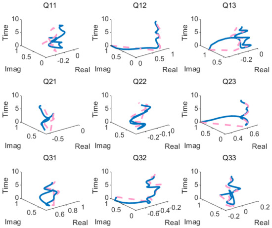
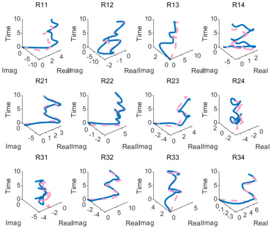
The above matrix is substituted into the BAFARNN model (4), OZNNN model (2) and NTZNN model to obtain their convergence accuracy. Figure 1, Figure 2 and Figure 3 show their convergence speeds and convergence accuracy, respectively, under the conditions of no noise, constant noise and sometimes variable noise. Table 2 records the detailed experimental data. Generally speaking, the number line can reflect the data more accurately [46]. Therefore, the number line is used in Figure 1, Figure 2, Figure 3 and Figure 4 to achieve a more pronounced contrast. The results show that the convergence time of the OZNN model (2) is 60 times that of the BAFARNN model (4), and the convergence time of the NTZNN model is 20 times that of the BAFARNN model (4). The experimental results show that the convergence performance of the BAFARNN model (4) is much better than that of the RNN model commonly used in DQRF (1). However, in a noisy environment, the convergence rate of the NTZNN model is prolonged, and it cannot reach a steady state in the experimental time. The convergence accuracy of OZNN (2) is much lower than that of the BAFARNN model (4), and the OZNN model (2) cannot converge in the case of time-varying noise. In contrast, the BAFARNN model (4) has excellent stability and robustness. In addition, we also analyzed the convergence of matrices and , and matrices and in Figure 4 in the noiseless environment. Their convergence is better than that of the OZNN model (2) and the NTZNN model.
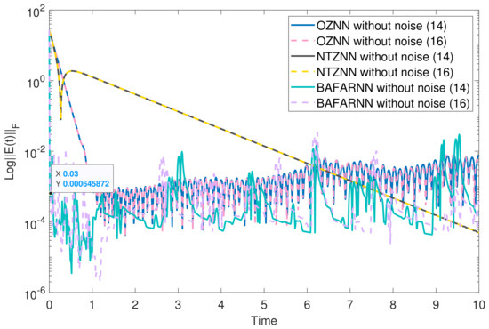
Figure 1.
The convergence accuracy (logarithm) of the model without noise. The design parameters are = 5, = 5 and = 4.
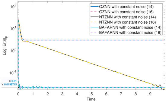
Figure 2.
The convergence accuracy (logarithm) of the model under constant noise. The design parameters are = 5, = 6 and = 6.
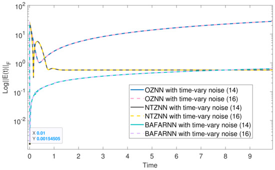
Figure 3.
The convergence accuracy (logarithm) of the model under time-varying noise. The design parameters are = 5, = 3 and = 3.
Table 2.
Comparison of three different ZNN models in terms of robustness and convergence time for solving time-varying DRQF.
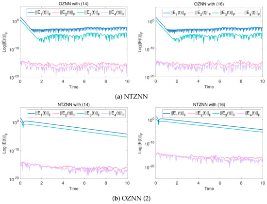
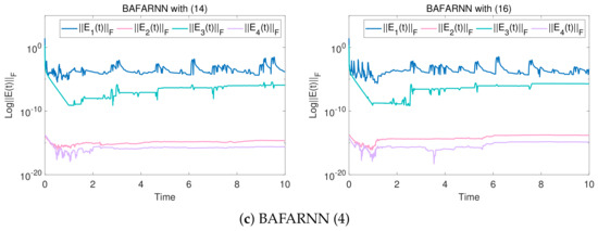
Figure 4.
When solving low-dimensional DQRF (1) in noiseless environments, matrices and , and matrices and , of six results from the three models are obtained. The design parameters are = 5, = 5 and = 4.
5.2. Numerical Simulation of High-Dimensional Complex Matrix
The high-dimensional matrix (t) is input. The noise is injected to observe its convergence. Where ,
All elements of are listed as below (Table 3).
Table 3.
matrix element expressions.
Then, the initial states of the other four matrices are given:
The above matrix is substituted into the BAFARNN model (4) and OZNN model (2) to obtain their convergence accuracy. Figure 5, Figure 6 and Figure 7 show their convergence speeds and convergence accuracy, respectively, under the conditions of no noise, constant noise and sometimes variable noise. Table 4 records the detailed experimental data. The results show that the convergence time of the OZNN model (2) is 80 times that of the BAFARNN model (4). The experimental results show that the convergence performance of the BAFARNN model (4) is much better than that of the RNN model commonly used in DQRF (1). In addition, we also analyze the convergence of matrices and , and matrices and in Figure 8 in the noiseless environment. Their convergence is better than that of the OZNN model (2) and the NTZNN model (Figure 9 and Figure 10).
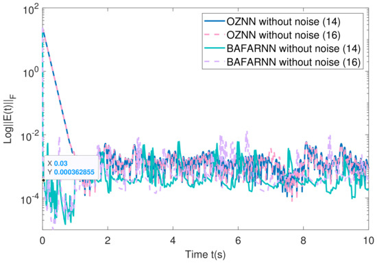
Figure 5.
The convergence accuracy (logarithm) of the model without noise. The design parameters are = 5, = 5 and = 4.
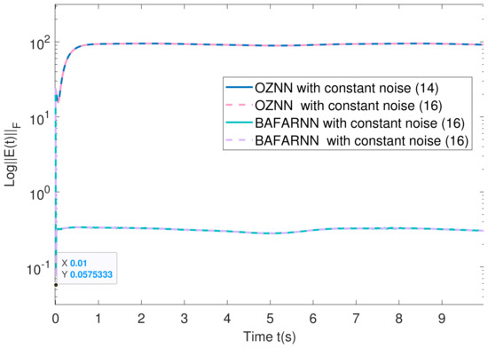
Figure 6.
The convergence accuracy (logarithm) of the model under constant noise. The design parameters = 5, = 4 and = 4.
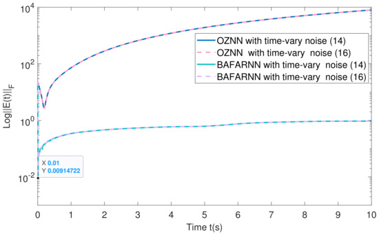
Figure 7.
The convergence accuracy (logarithm) of the model under time-varying noise. The design parameters = 5, = 4 and = 4.
Table 4.
Comparison of two different ZNN models in terms of robustness and convergence time for solving time-varying DRQF.
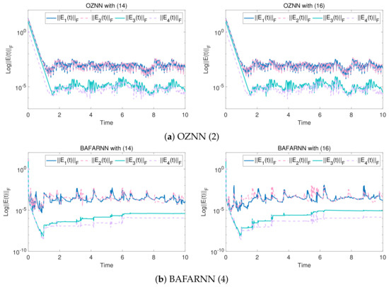
Figure 8.
When solving high-dimensional DQRF (1) in noiseless environments, matrices and , and matrices and , of four results from the two models are obtained. The design parameters are = 5, = 5 and = 4.
Remark 4.
Firstly, the example of 3D mobile target positioning in [20] helps us to understand that models such as BAFARNN, which use the ZNN model to deal with the DQRF, need to be time-varying linear. This is necessary in processing data provided by the mutual communication of sensor nodes. Additionally, some constraints are required, such as a limit on the time difference. Secondly, implementing the BAFARNN model requires techniques such as the Kronecker product and vectorization techniques to transform the model into a vector form that can be processed using MATLAB. The common implementation method ode45 in MATLAB is used for accurate experimental conclusions. Finally, all simulation experiments mentioned in this paper were conducted on an Intel®CoreTM i7-10510U CPU @ 1.80GHz 2.30 GHz computer with the Windows 11 operating system and MATLAB R2022a installed with 16 GB RAM.
6. Conclusions
This paper proposes a model to solve the DQRF based on coefficient consideration, the bounded adaptive function activated recurrent neural network (BAFARNN). It is worth noting that the bounded adaptive coefficient function (BACF) is innovative, and it is applied to the BAFARNN model. The BACF not only improves the convergence speed of the BAFARNN model but also improves the convergence accuracy. Moreover, the model has strong stability and excellent robustness under noisy environments. Moreover, the convergence and noise resistance of the BAFARNN model under constant and time-varying noise are demonstrated via a theoretical analysis of the new model. Ultimately, tests using simulation experiments are conducted on various aspects of the BAFARNN model to confirm its accuracy. As the parameters may vary, the suggested adaptive coefficient based on the ZNN model could be adjusted and applied in future research. In addition, the model can solve the DQRF in noisy environments and address various issues, such as numerical analysis and engineering applications.
Author Contributions
W.Y. and Y.G. are the co-first authors of the article. Conceptualization, W.Y. and X.X.; methodology, W.Y. and Z.S.; software, C.J. and Y.Z.; validation, C.J. and Y.Z.; writing—original draft preparation, W.Y. and Y.G.; writing—review and editing, C.J., Z.S. and Y.Z.; visualization, Z.S. and W.Y.; project administration, X.X. and Y.G.; funding acquisition, X.X. and Y.G. All authors have read and agreed to the published version of the manuscript.
Funding
This research was funded by Hainan Province Science and Technology Special Fund (No. ZDKJ202142).
Institutional Review Board Statement
Not applicable.
Informed Consent Statement
Not applicable.
Data Availability Statement
Not applicable.
Conflicts of Interest
The authors declare no conflict of interest.
References
- Zheng, Y.; Xu, A. Tensor completion via tensor QR decomposition and l2,1-norm minimization. Signal Process. 2021, 189, 108240. [Google Scholar] [CrossRef]
- Terao, T.; Ozaki, K.; Ogita, T. Lu-cholesky QR algorithms for thin QR decomposition. Parallel Comput. 2020, 92, 102571. [Google Scholar] [CrossRef]
- Zhou, X.; Dong, C.; Zhao, C.; Bai, X. Temperature-field reconstruction algorithm based on reflected sigmoidal radial basis function and QR decomposition. Appl. Therm. Eng. 2020, 171, 114987. [Google Scholar] [CrossRef]
- Dabbakuti, J.K.; Mallika, Y.; Rao, M.V.; Rao, K.R.; Ratnam, D.V. Modeling of GPS-TEC using QR-decomposition over the low latitude sector during disturbed geomagnetic conditions. Adv. Space Res. 2019, 64, 2088–2103. [Google Scholar] [CrossRef]
- Zhu, M.; Liang, D.; Yan, P. A point pattern matching algorithm based on QR decomposition. Optik 2014, 125, 3485–3490. [Google Scholar] [CrossRef]
- Shigeta, T.; Young, D.L.; Liu, C.-S. Adaptive multilayer method of fundamental solutions using a weighted greedy QR decomposition for the laplace equation. J. Comput. Phys. 2012, 231, 7118–7132. [Google Scholar] [CrossRef]
- Du, Z.; Niu, Z.; Fang, W. Block QR decomposition based power system state estimation algorithm. Electr. Power Syst. Res. 2005, 76, 86–92. [Google Scholar]
- Wang, K.; Chen, Z.; Ying, S.; Xu, X. Low-rank matrix completion via qr-based retraction on manifolds. Mathematics 2023, 11, 1155. [Google Scholar] [CrossRef]
- Sethi, A.; O’Donoghue, P.; Luthey-Schulten, Z. Evolutionary profiles from the qr factorization of multiple sequence alignments. Proc. Natl. Acad. Sci. USA 2005, 102, 4045–4050. [Google Scholar] [CrossRef]
- Sahoo, J.K.; Behera, R.; Stanimirović, P.S.; Katsikis, V.N. Computation of outer inverses of tensors using the QR decomposition. Comput. Appl. Math. 2020, 39, 1–20. [Google Scholar] [CrossRef]
- Mehra, I.; Nishchal, N.K. Fingerprint image encryption using phase retrieval algorithm in gyrator wavelet transform domain using QR decomposition. Opt. Commun. 2023, 533, 129265. [Google Scholar] [CrossRef]
- Rakheja, P.; Singh, P.; Vig, R. An asymmetric image encryption mechanism using QR decomposition in hybrid multi-resolution wavelet domain. Opt. Lasers Eng. 2020, 134, 106177. [Google Scholar] [CrossRef]
- Li, Z.; Zhang, Y.; Ming, L.; Guo, J.; Katsikis, V.N. Real-domain QR decomposition models employing zeroing neural network and time-discretization formulas for time-varying matrices. Neurocomputing 2021, 448, 217–227. [Google Scholar] [CrossRef]
- Ghaderyan, P.; Abbasi, A.; Ebrahimi, A. Time-varying singular value decomposition analysis of electrodermal activity: A novel method of cognitive load estimation. Measurement 2018, 126, 102–109. [Google Scholar] [CrossRef]
- Yanev, P.; Foschi, P.; Kontoghiorghes, E.J. Algorithms for computing the qr decomposition of a set of matrices with common columns. Algorithmica 2004, 39, 83–93. [Google Scholar] [CrossRef]
- Chen, T.; He, H.; He, C.; Chen, G. New parameter-identification method based on QR decomposition for nonlinear time-varying systems. J. Eng. Mech. 2019, 145, 04018118. [Google Scholar] [CrossRef]
- Katsikis, V.N.; Mourtas, S.D.; Stanimirović, P.S.; Zhang, Y. Continuous-time varying complex QR decomposition via zeroing neural dynamics. Neural Process. Lett. 2021, 53, 3573–3590. [Google Scholar] [CrossRef]
- Zhang, Y.; Yi, C. Zhang Neural Networks and Neural-Dynamic Method; Nova Science Publishers, Inc.: New York, NY, USA, 2011; Volume 1, pp. 1–261. [Google Scholar]
- Zhang, Y.; Ge, S.S. Design and analysis of a general recurrent neural network model for time-varying matrix inversion. IEEE Trans. Neural Netw. 2005, 16, 1477–1490. [Google Scholar] [CrossRef]
- Xiao, L.; He, Y.; Li, Y.; Dai, J. Design and analysis of two nonlinear znn models for matrix lr and qr factorization with application to 3d moving target location. IEEE Trans. Ind. Inform. 2022, 1–11. [Google Scholar] [CrossRef]
- Zhu, J.; Jin, J.; Chen, W.; Gong, J. A combined power activation function based convergent factor-variable ZNN model for solving dynamic matrix inversion. Math. Comput. Simul. 2022, 197, 291–307. [Google Scholar] [CrossRef]
- He, Y.; Xiao, L.; Sun, F.; Wang, Y. A variable-parameter ZNN with predefined-time convergence for dynamic complex-valued Lyapunov equation and its application to AOA positioning. Appl. Soft Comput. 2022, 130, 109703. [Google Scholar] [CrossRef]
- Jiang, C.; Xiao, X.; Liu, D.; Huang, H.; Xiao, H.; Lu, H. Nonconvex and bound constraint zeroing neural network for solving time-varying complex-valued quadratic programming problem. IEEE Trans. Ind. Inform. 2021, 17, 6864–6874. [Google Scholar] [CrossRef]
- Jiang, C.; Xiao, X. Norm-based adaptive coefficient znn for solving the time-dependent algebraic riccati equation. IEEE CAA J. Autom. Sin. 2023, 10, 298–300. [Google Scholar] [CrossRef]
- Xiao, L.; Zhang, Y.; Dai, J.; Chen, K.; Yang, S.; Li, W.; Liao, B.; Ding, L.; Li, J. A new noise-tolerant and predefined-time ZNN model for time-dependent matrix inversion. Neural Netw. 2019, 117, 124–134. [Google Scholar] [CrossRef]
- Liao, B.; Wang, Y.; Li, W.; Peng, C.; Xiang, Q. Prescribed-time convergent and noise-tolerant z-type neural dynamics for calculating time-dependent quadratic programming. Neural Comput. Appl. 2021, 33, 5327–5337. [Google Scholar] [CrossRef]
- Li, Z.; Liao, B.; Xu, F.; Guo, D. A new repetitive motion planning scheme with noise suppression capability for redundant robot manipulators. IEEE Trans. Syst. Man Cybern. Syst. 2020, 50, 5244–5254. [Google Scholar] [CrossRef]
- Yang, M.; Zhang, Y.; Hu, H. Discrete ZNN models of Adams-Bashforth (AB) type solving various future problems with motion control of mobile manipulator. Neurocomputing 2020, 384, 84–93. [Google Scholar] [CrossRef]
- Wu, D.; Zhang, Y. Discrete-time ZNN-based noise-handling ten-instant algorithm solving Yang-Baxter-like matrix equation with disturbances. Neurocomputing 2022, 488, 391–401. [Google Scholar] [CrossRef]
- Xiao, L.; Li, L.; Tao, J.; Li, W. A predefined-time and anti-noise varying-parameter ZNN model for solving time-varying complex stein equations. Neurocomputing 2023, 526, 158–168. [Google Scholar] [CrossRef]
- Zeng, Y.; Xiao, L.; Li, K.; Li, J.; Li, K.; Jian, Z. Design and analysis of three nonlinearly activated ZNN models for solving time-varying linear matrix inequalities in finite time. Neurocomputing 2020, 390, 78–87. [Google Scholar] [CrossRef]
- Luo, J.; Yang, H.; Yuan, L.; Chen, H.; Wang, X. Hyperbolic tangent variant-parameter robust ZNN schemes for solving time-varying control equations and tracking of mobile robot. Neurocomputing 2022, 510, 218–232. [Google Scholar] [CrossRef]
- Ren, X.; Yue, C.; Ma, T.; Wang, J.; Wang, J.; Wu, Y.; Weng, Z. Adaptive parameters optimization model with 3D information extraction for infrared small target detection based on particle swarm optimization algorithm. Infrared Phys. Technol. 2021, 117, 103838. [Google Scholar] [CrossRef]
- Lv, L.; Zhao, L.; Li, H. Design of adaptive parameter observer and laser network controller based on sliding mode control technology. Optik 2022, 257, 168790. [Google Scholar]
- Jiang, C.; Wu, C.; Xiao, X.; Lin, C. Robust neural dynamics with adaptive coefficient applied to solve the dynamic matrix square root. Complex Intell. Syst. 2022. [Google Scholar] [CrossRef]
- Wu, Y.; Li, Y.; Feng, S.; Huang, M. Pansharpening using unsupervised generative adversarial networks with recursive mixed-scale feature fusion. IEEE J. Sel. Top. Appl. Earth Obs. Remote. Sens. 2023, 16, 3742–3759. [Google Scholar] [CrossRef]
- Chen, C.; Lu, J. Data-driven adaptive compensation control for a class of nonlinear discrete-time system with bounded disturbances. ISA Trans. 2022, 135, 492–508. [Google Scholar] [CrossRef]
- Yue, J.; Liu, L.; Gu, N.; Peng, Z.; Wang, D.; Dong, Y. Online adaptive parameter identification of an unmanned surface vehicle without persistency of excitation. Ocean Eng. 2022, 250, 110232. [Google Scholar] [CrossRef]
- Jia, L.; Xiao, L.; Dai, J.; Qi, Z.; Zhang, Z.; Zhang, Y. Design and application of an adaptive fuzzy control strategy to zeroing neural network for solving time-variant QP problem. IEEE Trans. Fuzzy Syst. 2021, 29, 1544–1555. [Google Scholar] [CrossRef]
- Song, Z.; Lu, Z.; Wu, J.; Xiao, X.; Wang, G. Improved ZND model for solving dynamic linear complex matrix equation and its application. Neural Comput. Appl. 2022, 34, 1–14. [Google Scholar] [CrossRef]
- Auckenthaler, T.; Huckle, T.; Wittmann, R. A blocked qr-decomposition for the parallel symmetric eigenvalue problem. Parallel Comput. 2014, 40, 186–194. Available online: https://www.sciencedirect.com/science/article/pii/S0167819114000404 (accessed on 13 March 2023). [CrossRef]
- Cosnard, M.; Muller, J.M.; Robert, Y. Parallel qr decomposition of a rectangular matrix. Numer. Math. 1986, 48, 239–249. [Google Scholar] [CrossRef]
- Brewer, J. Kronecker products and matrix calculus in system theory. IEEE Trans. Circuits Syst. 1978, 25, 772–781. [Google Scholar] [CrossRef]
- Penrose, R. On best approximate solutions of linear matrix equations. Math. Proc. Camb. Philos. Soc. 1956, 52, 17–19. [Google Scholar] [CrossRef]
- Fox, H.; Bolton, B. (Eds.) 6—Laplace transform. In Mathematics for Engineers and Technologists; IIE Core Textbooks Series; Butterworth-Heinemann: Oxford, UK, 2002; pp. 198–234. [Google Scholar]
- Fowler, S.; Stanwick, V. (Eds.) Chapter 10—Designing graphs and charts. In Web Application Design Handbook; Interactive Technologies; Morgan Kaufmann: San Francisco, CA, USA, 2004; pp. 265–323. [Google Scholar]
Disclaimer/Publisher’s Note: The statements, opinions and data contained in all publications are solely those of the individual author(s) and contributor(s) and not of MDPI and/or the editor(s). MDPI and/or the editor(s) disclaim responsibility for any injury to people or property resulting from any ideas, methods, instructions or products referred to in the content. |
© 2023 by the authors. Licensee MDPI, Basel, Switzerland. This article is an open access article distributed under the terms and conditions of the Creative Commons Attribution (CC BY) license (https://creativecommons.org/licenses/by/4.0/).