Abstract
This paper investigates the optimal private health insurance contract design problem, considering the joint interests of a policyholder and an insurer. Both the policyholder and the insurer jointly determine the premium of private health insurance. In order to better reflect reality, the illness expenditure is modelled by an extended compound Poisson process depending on health status. Under the mean–variance criterion and by applying dynamic programming, control theory, and leader–follower game techniques, analytically time-consistent private health insurance strategies are derived, optimal private health insurance contracts are designed, and their implications toward insurance are analysed. Finally, we perform numerical experiments assuming that the policyholder and the insurer calculate their wealth every year and they deposit their disposable income into the Bank of China with the interest rate being . The values of other model parameters are set by referring to the data in the related literature. We find that the worse the policyholder’s health, the higher the premium that they pay for private health insurance, and buying private health insurance can effectively reduce the policyholder’s economic losses caused by illnesses.
Keywords:
illness expenditure; leader–follower game; premium; private health insurance; stochastic optimal control MSC:
62P05; 91B28; 93E20
JEL Classification:
G11; G22; C61
1. Introduction
Health insurance, consisting of both social health insurance and private health insurance in most countries, is very important for reducing economic losses. In practice, due to the influence of many factors, social health insurance can only reimburse partial expenditures of illnesses. As an important supplement to social health insurance, private health insurance has recently attracted increasing attention.
Recently, quite a few scholars have investigated issues surrounding private health insurance. Ref. [1] investigated private health insurance in Germany, where the ex post moral hazard was considered. Ref. [2] analysed the evolution of private health insurance expenditure in Spain. Ref. [3] investigated selection bias and the moral hazard problem in the Australian private health insurance market. Ref. [4] examined the driving force behind the rise of private health insurance in Sweden. Ref. [5] considered the causal effect of private health insurance in Brazil. Ref. [6] analysed the development trends and determinants of private health insurance in Ireland. These studies examined private health insurance from an empirical perspective, which can only reflect individual-based problems in private health insurance.
Mathematical models have also been adopted to study private health insurance from a quantitative perspective. Mathematical formulation is the basic concept used by many researchers when conducting various studies. It provides prediction results before experimental investigation. However, it may be very difficult to solve some realistic problems when using mathematical formulation, and it is prone to miscalculations (see [7,8,9] for details). Ref. [10] constructed a model of non-linear health insurance and analysed its properties. Ref. [11] quantitatively described selection behaviours of patients and physicians, and then studied the resulting optimal insurance problem. Ref. [12] considered the optimal design of health insurance policies. Ref. [13] proposed a generalized hierarchical Bayesian collective model and then predicted the premium. Ref. [14] used a Markov chain to describe the health status of a policyholder and applied it to estimate the technical basis for private health insurance policies. Ref. [15] studied the construction of medical inflation indexes and the formulation of premiums of lifelong health insurance. The above-mentioned studies were based on static or discrete-time frameworks; however, they cannot reflect a continuous change in illness information and health status. Therefore, it is more reasonable to study health insurance problem from a continuous-time perspective. As far as we know, there are few studies in this field. Ref. [16] studied private health insurance covering critical illnesses in a continuous-time consumption-investment problem. However, the author did not consider other illnesses.
In the current literature on private health insurance, the optimal private health insurance contract design problem has been rarely studied. If we enter the topic “optimal private health insurance contract design” into Web of Science, we only obtain ten references. These ten references may not all study the optimal private health insurance contract design problem. Designing an optimal private health insurance contract is beneficial for both the policyholder and the insurer because the policyholder can reduce the losses caused by illnesses and the insurer can earn a higher premium. Ref. [17] considered the single-period private health insurance contract design problem. However, the authors only considered the interests of the policyholder. In practice, a private health insurance contract involves both the interest of an insurer and that of a policyholder, with conflicting interests. A policyholder pays a premium to an insurer and hopes to receive an indemnity from the insurer when illnesses occur; an insurer undertakes the risk of a policyholder’s illness in exchange for the policyholder’s payment of premium. Therefore, the insurer is a participant in the private health insurance contract; however, their decisions were ignored in [17]. Ref. [18] studied the Pareto-optimal insurance policy, where the joint interests of an insurer and a policyholder were considered. However, health insurance is different from other forms of insurance. This is because the policyholder’s health status affects the formulation of the health insurance contract. To the best of our knowledge, there is no existing literature that examines the optimal design of a private health insurance contract considering the joint interests of the policyholder and the insurer.
The level of illness expenditure has an important influence on the decision-making of a policyholder and an insurer. Therefore, illness expenditure is closely related to the design of a private health insurance contract. However, it is complicated and difficult to predict illness expenditure in reality. Recently, [19,20,21] adopted a Poisson regression model to predict illness expenditure. However, these studies only considered the prediction of static illness expenditure. In practice, the prediction of dynamic illness expenditure is more relevant as illness expenditure is constantly changing. It may be very difficult to choose an appropriate stochastic process to predict dynamic illness expenditure. The Poisson process may be a good choice; recently, [22] adopted the Poisson process to describe the number of illnesses, and used the compound Poisson process to describe the cumulative expenditures of illnesses. Nevertheless, this method cannot reflect the influence of health status on illness expenditure. As we know, health status almost surely affects illness expenditure. For example, a healthy person and an otherwise healthy smoker probably have different illness expenditures when respiratory illnesses occur. Consequently, it is quite important for us to consider the impact of health status on illness expenditure for an accurate modelling of reality.
Based on the state of the current research, the optimal private health insurance contract design problem is studied in this article. Because private health insurance information and health states change dynamically, a continuous-time model is adopted; this is different from the single-period model considered in [17]. In view of the successful application of the Poisson process and inspired by the empirical studies of [19,20,21], it is assumed that the number of illnesses follows some kind of Poisson process. From some real data (https://www.cpc.unc.edu/projects/china (accessed on 17 April 2023), https://chfs.swufe.edu.cn/ (accessed on 17 April 2023), http://charls.pku.edu.cn/index.html (accessed on 17 April 2023), we found that there is no significant dependency between individual or family illness expenditures at different times. The reason for this may be that the expenditures of different illnesses at different times are independent. Therefore, this article assumes that the one-time expenditures of illnesses are mutually independent. Moreover, to reflect the influence of health status on illness expenditures, this article assumes that health status can be simulated by a Markov chain. The Markov chain simultaneously modulates the number of illnesses and the one-time illness expenditure. In the end, we adopt an extended compound Poisson process depending on health status to simulate the cumulative expenditures of illnesses. This generalizes the model considered in [22]. Furthermore, the joint interests of the policyholder and the insurer are considered. That is, the policyholder and the insurer jointly determine the premium of a private health insurance contract. In insurance practice, a policyholder signs a private health insurance contract with the hope that an insurer can share partial expenditure of their illnesses. Therefore, this article assumes that the policyholder determines the sharing strategy regarding illness expenditure. Meanwhile, because the insurer bears partial expenditure of the policyholder’s illnesses, they determine the premium strategy in order to receive the highest possible premium through bargaining with the policyholder. With this, the illness expenditure sharing strategy and the decision on the highest receivable premium jointly determine the private health insurance premium. Under the mean–variance criterion and by applying dynamic programming, control theory and leader–follower game techniques, analytically time-consistent private health insurance strategies are derived, optimal private health insurance contracts are designed, and their implications on insurance are analysed. Finally, numerical experiments are carried out and the theoretical results are explained.
The main contributions of this article include: (1) A continuous-time private health insurance problem is investigated that can better reflect the dynamic changes in the private health insurance information and the health status. (2) An extended compound Poisson process model of illness expenditure is introduced, which depends on health status. This can effectively describe the influence of health status on the private health insurance contract. (3) An optimal private health insurance contract with consideration of the joint interests of a policyholder and an insurer is designed. This is more in line with actual private health insurance in reality. (4) An explicit optimal private health insurance contract is derived, which can guide practical private health insurance more effectively. (5) We numerically discuss the influences of health status and key model parameters on the optimal private health insurance contract and analyse the influence of private health insurance on the policyholder. The results reveal some meaningful phenomena and provide important guidance for buying private health insurance in practice.
The remainder of this paper is organized as follows. In Section 2, a new framework for the private health insurance contract design is proposed. In Section 3, the game framework for designing the optimal private health insurance contract is provided. In Section 4, the policyholder’s best response strategy is derived. The insurer’s optimal strategy is obtained in Section 5. In Section 6, the optimal private health insurance contract is deduced. The numerical results are provided in Section 7. The final section summarizes the paper.
2. Private Health Insurance Contract
In this section, a new framework for private health insurance considering the joint interests of the policyholder and the insurer is proposed. To be mathematically rigorous, we assume that all the random variables and stochastic processes are defined on a filtered probability space satisfying the usual conditions. That is, is right continuous and complete with respect to the probability measure , is the terminal time for private health insurance contract, and stands for the information available up to time , which is an augmented filtration generated by a martingale , a Markov chain , and a compound Poisson process . For a detailed introduction and some possible choices for the filtration , one can refer to [23].
In health insurance, many countries divide the health status of a policyholder into multiple levels. For example, the United States divides health status into preferred plus/preferred elite, preferred, preferred smoker, standard plus, standard smoker, and substandard. Different health statuses affect the illness expenditure and the premium of health insurance. To model this relationship, let denote the finite health status space. The health status is described through a continuous-time and finite state Markov chain . It takes the value in the state space . Similar to [24], let denote the -matrix of such that , for , . Furthermore, the Markov chain has the following semi-martingale representation
where is some -valued martingale, and denotes the transpose of .
Remark 1.
We, for the first time, use a continuous-time and finite state Markov chain to define health status. This can better reflect the change in health status and is more consistent with an actual health situation.
Considering the influence of health status on illness expenditure and inspired by [22], this article constructs an extended compound Poisson process depending on health status, and uses it to describe the cumulative illness expenditures. The concrete construction method is as follows.
Suppose that under health status , the number of illnesses follows a Poisson process with the intensity being , and is the expenditure of the jth illness under the health status . According to the principles we demonstrated in the introduction and referring to the insurance practice, we assume that forms a sequence of independent and identically distributed non-negative random variables with a common distribution function . Here, is the common random variable of . To be consistent with practice, we assume that and . Obviously, the extended compound Poisson process depends on health status and represents the cumulative expenditures of illnesses in the time interval .
Remark 2.
Although both this article and [22] use the compound Poisson process to define the cumulative expenditures of illnesses, there are some significant differences between them. Importantly, in our compound Poisson process, both the expenditure of each illness and the number of illnesses depend on the health status. Therefore, the compound Poisson process defined here is more reasonable.
To reduce the financial losses caused by illnesses, one can buy private health insurance. We assume that the retention proportion of a policyholder for the expenditures of illnesses under health status is , and the rest of the illness expenditures are paid by an insurer. Here denotes the expenditure of the illness sharing strategy, and it is the policyholder’s private health insurance decision variable.
Because the insurer bears of each illness’ expenditure, the policyholder needs to pay a premium to the insurer. In practice, the premium is usually related to the disposable income of a policyholder; if the required premium exceeds the affordability of the policyholder, they may not sign the private health insurance contract. For this reason, we assume that the premium is some proportion of the disposable income of the policyholder. Inspired by the methods for determining the contribution premium in pension fund (for example, [25]), we assume that the cumulative disposable income of a policyholder in the time interval , depending on health status , satisfies . Here, is the change rate of the disposable income, and it is a bounded function. As we illustrated in the introduction, the policyholder and the insurer jointly determine the premium. More specifically, in reference to the health insurance practice rules in countries such as China, the premium paid by the policyholder per unit time is . Here, stands for the proportion of disposable income that the insurer hopes to receive. In what follows, is called the insurer’s private health insurance strategy.
Remark 3.
The reasons for setting the premium to are as follows. Firstly, a similar proportional premium principle has been frequently adopted for an insurer’s reinsurance decision; for example, [24,26,27,28] considered the proportional premium principle. Inspired by this idea, we introduce the proportional private health insurance premium here. Secondly, the premium received by an insurer should depend on the health status and illness expenditure they bear. The insurer pays of each illness’ expenditure. Hence, the coefficient affects the premium. Thirdly, the premium should reflect an insurer’s interest. When the insurer bears the entire illness expenditure, i.e., , the premium becomes , which reflects the insurer’s highest demand for premium in some sense. The insurer can negotiate with the policyholder by adjusting . Last but not least, the proposed premium pattern can reflect the joint interests of the policyholder and the insurer in the sense that is determined by the policyholder and is determined by the insurer.
A private health insurance contract consists of the policyholder’s strategy and the insurer’s strategy .
When signing the private health insurance contract, the policyholder and the insurer are allowed to invest their respective wealth in the risk-free asset with the interest rate to increase their wealth. Then, the policyholder’s wealth dynamics can be expressed as
with the initial wealth being , and the insurer’s wealth dynamics can be expressed as
with the initial wealth being .
Remark 4.
From (1) and (2), we can find that we consider the joint interests of both the policyholder and the insurer simultaneously. The interests of the policyholder and the insurer are reflected by the strategies and , respectively. To the best of our knowledge, the joint interests of the policyholder and the insurer in the continuous-time health insurance problem are considered here for the first time.
To determine the optimal private health insurance contract, we define an admissible strategy as follows.
Definition 1.
(Admissible Strategy). The strategies and where are said to be admissible if they satisfy the following conditions:
- (i)
- and are progressively measurable with respect to ;
- (ii)
- For any , and .
The sets of all admissible strategies and are denoted by and , respectively.
Now, we try to find the solutions to Equations (1) and (2). The Poisson random measure on can be used to represent the compound Poisson process as
We denote by , then
Here, is the compensator of the random measure . The compensated measure is then related to the compound Poisson process as follows
3. Game Problem Formation
Firstly, we construct the objective functions for the policyholder and the insurer under the mean–variance (MV) criterion; then, based on the leader-follower game theory, we present the game framework for designing the optimal private health insurance contract.
Let and denote the terminal wealth of the policyholder and the insurer under the strategies and . According to the MV criterion, the corresponding objective functions and under the initial wealth and health status can be defined as
and
Here, and are the risk aversion coefficients of the policyholder and the insurer, respectively; , , and .
During the process of developing a private health insurance contract in insurance practice, the status of a policyholder is different from that of an insurer. This is because the insurer’s economic strength is usually stronger than that of the policyholder. Therefore, the insurer should be the leader and the policyholder should be the follower. Based on this observation, the objectives of the policyholder and the insurer can be described as follows, respectively.
For any given strategy of the insurer, the objective of the policyholder is to find a strategy such that
Here, is the policyholder’s best response strategy with respect to given . With respect to the strategy chosen by the policyholder, the objective of the insurer is to find a strategy such that
where . The pair forms the optimal strategy to problems (11) and (12), which is called the optimal private health insurance contract. Correspondingly, the policyholder’s optimal value function is , and the insurer’s optimal value function is .
It is not difficult to see from (11) and (12) that the optimal private health insurance contract can be derived as follows. Firstly, the insurer announces their strategy . Secondly, the policyholder observes the insurer’s strategy and chooses their best response strategy with respect to in order to maximize . Thirdly, the insurer learns that the policyholder would execute the strategy ; they then choose a strategy such that is maximized. Finally, the policyholder adjusts their strategy according to the insurer’s optimal strategy and forms their optimal strategy . In other words, the insurer is the leader and the policyholder is the follower, and the determination process of the private health insurance contract is a game between the leader and the follower.
Time consistency is a basic requirement for rational decision-making under many situations. Due to the conditional variance term in their objective functions, problems (11) and (12) are time inconsistent. Thus, we will find a time-consistent strategy for the policyholder and the insurer in Section 4 and Section 5, respectively.
4. The Policyholder’s Best Response Strategy
For any chosen by the insurer, the policyholder’s best response strategy is derived in this section. To this end, inspired by [29], we define the following equilibrium strategy and corresponding equilibrium value function for the policyholder. Note that the optimal time-consistent strategy will coincide with the equilibrium strategy and the usual optimal value function will be the equilibrium value function.
Definition 2.
For given , any initial state and real number , we define the following strategy
If
then is called an equilibrium strategy, the corresponding equilibrium value function is .
For simplicity, we introduce the following two notations.
where is a constant.
For any , we define the infinitesimal generator for (1) as follows
Now, we present the verification theorem which ensures the optimality of the strategy obtained for problem (11).
Theorem 1.
(Verification theorem). For the wealth process (1), suppose there exist two real functions satisfying the following extended Hamilton–Jacobi–Bellman (HJB) equations: ,
here,
If , then is the policyholder’s time-consistent best response strategy, is the corresponding value function, and is the expected value of the terminal wealth.
Proof.
The proof consists of the following two steps.
Step 1 For any , define a stopping time sequence , , as follows
By applying Itô’s lemma to and utilizing the expression of , we obtain
By taking the conditional expectation on both sides of (16), we obtain
Because , we have according to (8) that for all
With (18), applying the dominated convergence theorem, setting n to infinity, and thus setting s to T in (17), we obtain
Analogously, by using It lemma to , we obtain
Similar to that as for (19), by applying It lemma to , we obtain
Step 2 We first introduce some notations and rewrite defined in (9) as
where and . , and are defined by
From the above equation, we obtain
Discretizing the above inequality with respect to any gives us that
This is equivalent to
On the other hand, for an arbitrary admissible strategy , we can construct a control strategy such as that in Definition 2. Applying at the time points t and , respectively, we obtain
where
Because on , we have by continuity that , and because on , we have
Therefore, we conclude that
This completes the proof. □
The following lemma presents the structure of the solutions to the extended HJB Equations (14) and (15). Because the proof is similar to that of Lemma 4.1 in [30], the details are omitted.
Lemma 1.
and have the following forms
Now, we can obtain the main results in this section.
Theorem 2.
The policyholder’s time-consistent best response strategy is ; here, is given by
and the corresponding value function is given by
where
and is the conditional expectation given under , .
Proof.
From Lemma 1, we have the following partial derivatives
With Definition 1, Theorem 1, and the fact that is concave with respect to , setting shows that the maximum point of is given by (32). Furthermore, we can obtain that the policyholder’s time-consistent best response strategy is by considering the constraints and the concavity of .
Substituting into (15), we have
From (32), we can see that . According to the definition of the private health insurance premium, is positively correlated with the private health insurance premium. This means that while purchasing a private health insurance can reduce the losses caused by illnesses, it is nonetheless costly, because the policyholder needs to pay more premium to the insurer. Therefore, when increases, the policyholder would increase the retention proportion in order to reduce the premium. This tells us that if the insurer raises the premium, the policyholder’s willingness to buy private health insurance would decrease. This is consistent with the practice in health insurance.
From (32), we can also see that and . These results demonstrate that with the increase in the illness expenditure, the policyholder’s willingness to buy private health insurance would increase. This is consistent with reality because the expenditure of illnesses is generally larger than the premium of a private health insurance. In other words, buying private health insurance can help reducing the losses caused by illnesses.
5. The Insurer’s Optimal Strategy
Once the insurer knows that the policyholder would execute the strategy , they will seek an optimal time-consistent strategy. Similar to Section 4, we first define the equilibrium strategy and equilibrium value function for the insurer as follows.
Definition 3.
For any given real number and initial state , we define the following strategy
If
then is called an equilibrium strategy for the insurer, and is the corresponding equilibrium value function.
Similar to the previous section, we call the above equilibrium strategy and equilibrium value function to be the insurer’s optimal time-consistent private health insurance strategy and optimal value function, respectively.
For a chosen strategy and any , the infinitesimal generator for the wealth process (2) is defined as
Parallel to Theorem 1 and Lemma 1, we have the following conclusions.
Theorem 3.
For the wealth process (2), suppose there exist two real functions satisfying the following extended HJB equations: ,
here,
If , then is the insurer’s optimal time-consistent private health insurance strategy, is the corresponding value function, and is the expected value of the terminal wealth.
Lemma 2.
and in Theorem 5.1 have the following forms
and
Based on Theorem 3 and Lemma 2, we can obtain the optimal solution to problem (12), which is shown in the following theorem.
Theorem 4.
With respect to the policyholder’s best response strategy , the insurer’s optimal time-consistent private health insurance strategy is . Here is given by
and the corresponding value function is given by
where
Proof.
When , we can rewrite the extended HJB Equation (40) as
From Lemma 2, we have the following partial derivatives
Substituting (42), (43), and (50) into (49), we obtain, after some simplifications, that
where is given by (48).
With Definition 1, Theorem 3, and the fact that is concave with respect to , setting tells us that the maximum point of is given by (44). Furthermore, we can deduce that the insurer’s optimal time-consistent private health insurance strategy is by considering the constraints and the concavity of .
Substituting into (51), we obtain
Remark 6.
means that the policyholder pays all the expenditures of illnesses by herself, i.e., they do not sign the private health insurance contract with the insurer. This case is not the focus of this paper. On the other hand, means that the insurer would reimburse all the expenditures of illnesses. In practice, the insurer only reimburses some percentage of illness expenses. Therefore, this case can hardly happen in reality. Meanwhile, the solution processes of problem (12) for the cases and , respectively, are similar to that of . To avoid repetition and to be more consistent with reality, we omit these two extreme cases in Theorem 4.
6. Optimal Private Health Insurance Contract
Based on the results in Section 4 and Section 5, the optimal private health insurance contract is determined in this section.
Theorem 5.
The optimal private health insurance contract can be classified into the following two cases:
Case I: When
the optimal private health insurance contract is
Case II: When
the optimal private health insurance contract is
Proof.
When
we obtain from Theorem 4 that the insurer’s optimal time-consistent private health insurance strategy is . Substituting into (32), we find that the policyholder’s optimal time-consistent private health insurance strategy is
When
we obtain from Theorem 4 that the insurer’s optimal time-consistent private health insurance strategy is given by (55). Substituting (55) into (32), we obtain that the policyholder’s optimal time-consistent private health insurance strategy is given by (56). □
Case I seldom occurs in practice. When , the premium achieves its theoretical maximum value for given . Usually, when this happens, the policyholder would bargain with the insurer to reduce the premium.
The reason why the policyholder’s optimal private health insurance strategy becomes a constant in Case II is as follows. It can be seen from (32) that if the insurer’s strategy is a given constant, the policyholder’s optimal strategy will increase with respect to t. This means that the private health insurance demand and, thus, the insurer’s profit would decrease in t. This situation can only occur when the insurer passively accepts the policyholder’s decision and does not bargain with the policyholder. Under our game framework, the insurer has the bargaining power. To obtain a larger insurance share or a higher profit, the insurer would dynamically decrease the highest premium that they are hoping to receive from the private health insurance but does not passively accept the decreasing insurance share allocated by the policyholder. As a result, the policyholder always reserves a constant strategy, which is fully determined by the risk aversion coefficients of the policyholder and the insurer.
From Theorem 5, we can see that the policyholder’s health status has some influence on the optimal private health insurance contract. This is different from the usual insurance or reinsurance contract problem. In the ordinary insurance problem (for example, [18]), or reinsurance contract problem (for example, [33,34,35]), the health status has no influence on the insurance or reinsurance contract.
Now, we analyse the influence of and on the optimal private health insurance contract under Case II. From (55) and (56), we obtain that
Therefore, and are increasing and decreasing with respect to , respectively. Here, is the policyholder’s risk aversion coefficient. With an increase in , the policyholder is more willing to buy private health insurance, and thus transfers more illness expenditures to the insurer. Realizing that the policyholder would transfer more illness expenditures, the insurer adjusts their strategy to increase the premium.
From (55) and (56), we also obtain that
Therefore, both and are increasing with respect to . Here, is the insurer’s risk aversion coefficient. With an increase in , the insurer seeks to reduce the risk of potential illnesses. One direct way to accomplish this is to further increase the highest possible premium of their optimal strategy so as to reduce the illness expenditure transferred by the policyholder. Realizing that the insurer would increase the premium, the policyholder then increases the retention proportion of illness expenditure so as to reduce the premium they need to pay.
The above analyses show how the risk aversion coefficients affect the optimal private health insurance contract. We can also examine the influence of the private health insurance on the policyholder. To this end, we first derive the policyholder’s optimal value functions for the two cases: buying and not buying private health insurance. When the policyholder participates in private health insurance, under Case II, (because Case I is an extreme case and seldom happens in practice, we only consider the general case here, i.e., Case II) we obtain from (33) that the policyholder’s optimal value function is
where
and .
When the policyholder does not buy private health insurance, i.e., and , we have from (33) that the policyholder’s optimal value function becomes
where
We can examine the influence of the private health insurance on the policyholder by comparing and , which will be performed numerically in the next section.
7. Numerical Experiments
In this section, we first examine the effects of health status and model parameters on the optimal private health insurance contract and then analyse the influence of private health insurance on the policyholder.
We assume that the policyholder has three health states, i.e., the preferred (), the standard plus (), and the substandard (). Similar to [25], we assume that the growth rate of the disposable income satisfies . Referring to the data in [25], we set and . Without loss of generality, we assume that the expenditure of illnesses obeys the exponential distribution with parameter . Considering that as health condition becomes worse, the private health insurance premium rises, we assume that . Considering that as health condition becomes worse, illness expenditure also increases, we assume that , . In addition, we assume that the policyholder and the insurer calculate their wealth every year, i.e., months, and they deposit their disposable income into the Bank of China. The initial time is , the initial wealth is , and the interest rate is . It is quite difficult to obtain the real data for other parameters such as , , , . We chose their values by referring to the relevant studies such as [19,20,22]. Concretely, , , , . The -matrix is given as
7.1. Effects of Model Parameters and Health Status on the Optimal Private Health Insurance Contract
To facilitate the application of the obtained results, we examine the effects of model parameters and health status on the optimal private health insurance contract in this subsection. Because Case I in Theorem 5 is an extreme case, we only discuss the Case II in Theorem 5.
First, we assume that the health status of the policyholder is the preferred health status, that is, , as an example to analyse the influence of model parameters on the optimal private health insurance contract.
Figure 1 shows the effects of and on the optimal private health insurance contract. We can see from Figure 1a that and are increasing and decreasing, respectively, with respect to . These findings are consistent with our theoretical results in the last section. More importantly, we find that the private health insurance premium is increasing with respect to . With an increase in , the policyholder would purchase more private health insurance to diversify their health risks. This means that the policyholder intends to sign a private health insurance contract. Therefore, the result of the game between the policyholder and the insurer is an increase in the private health insurance premium. We find from Figure 1b that and are both increasing with respect to . These findings are also consistent with our theoretical results in the previous section. Furthermore, we find that the private health insurance premium is decreasing with respect to . When increases, the insurer is unwilling to sign a private health insurance contract. This leads the insurer to increase the price of the private health insurance premium. Hence, the result of the game between the policyholder and the insurer is a decrease in the private health insurance premium.
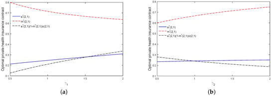
Figure 1.
Effects of and on the optimal private health insurance contract (a,b).
Figure 2 further examines the joint effects of and on the optimal private health insurance contract. From Figure 2a,b, it is clear that (resp. ) is more sensitive to (resp. ) than that to (resp. ). This implies that the insurer and the policyholder are more sensitive to the other’s risk aversion degree. The reason may be that the other party’s risk aversion coefficient corresponds to the uncertainty of the private health insurance premium. We can see from Figure 2c that is more sensitive to than to . This is due to the fact that the policyholder is the payer of the private health insurance premium, whereas the insurer is the receiver of the private health insurance premium.
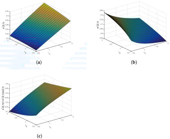
Figure 2.
Joint effects of and on the optimal private health insurance contract (a–c).
Now, we examine the effects of the health status and , on the private health insurance premium. The results are presented in Figure 3.
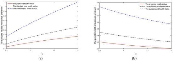
Figure 3.
Effects of the health status and , on the private health insurance premium (a,b).
From Figure 3, we can find that under three health states, the private health insurance premiums are increasing and decreasing with respect to and , respectively. This is consistent with what we obtained from Figure 1 and Figure 2. More importantly, as we can see from Figure 3, the premium of the private health insurance monotonically increases with the deterioration of the health condition from , to . Under poor health situation, people prefer to buy private health insurance to avoid economic losses caused by illnesses. Therefore, the policyholder will pay more private health insurance premium in this situation.
7.2. Influence of Private Health Insurance on the Policyholder
In this subsection, we analyse the influence of private health insurance on the policyholder. To avoid repetition, we only report the results under the health status . The influence of private health insurance on the policyholder is examined by comparing the optimal value function of a policyholder who buys private health insurance with the optimal value function of a policyholder who does not buy the private health insurance. and are determined by (58) and (59), respectively.
Figure 4a displays the effect of on and . We can see from Figure 4a that, whether the policyholder buys private health insurance or not, the change trends of and with respect to are consistent. Here, stands for the intensity of the number of illnesses. As becomes larger, the policyholder bears more illness expenditure the policyholder. Therefore, and monotonically decrease with respect to .
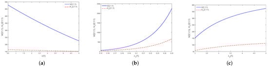
Figure 4.
Effects of , , and on and (a–c).
Figure 4b,c illustrate the effects of and on the optimal value functions and . Here, and stand for the growth intensity of the disposable income and the parameter of exponential distribution of illness expenditure. As becomes larger, the policyholder will have more the disposable income. Hence, and are increasing with respect to . As becomes larger, illness expenditure will decrease. This would lead to a decrease in the willingness of a policyholder to buy private health insurance. Therefore, the premium of the private health insurance becomes smaller, and thus and are increasing with respect to .
Further analysing Figure 4, we find that is always larger than . This shows that participating in private health insurance is helpful for avoiding the policyholder’s economic losses caused by illnesses.
Figure 5 and Figure 6 demonstrate the joint effects of and on and , respectively. We find that (resp. ) is decreasing and increasing with respect to and , respectively. These are consistent with what we obtained from Figure 4a,b. More importantly, it can be seen from Figure 5 and Figure 6 that and are more sensitive to than to . This tells us that whether a person participates in private health insurance or not, their disposable income has a more significant impact on the policyholder than that of the incidence intensity of illness. This is natural because the disposable income determines whether a person participates in private health insurance and the amount of private health insurance premiums paid.
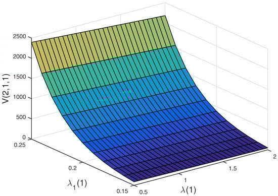
Figure 5.
Joint effects of and on .
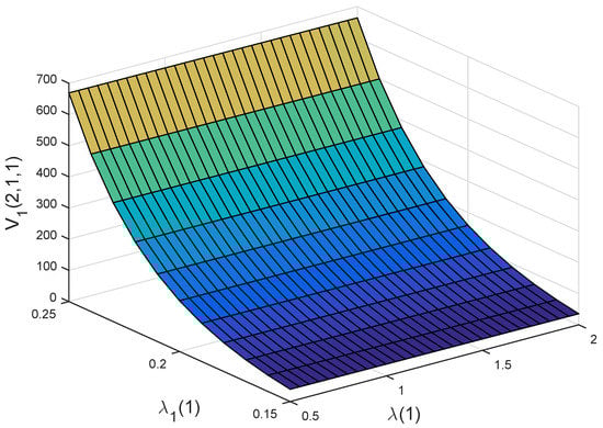
Figure 6.
Joint effects of and on .
Figure 7 and Figure 8 illustrate the joint effects of and on and , respectively. We find that (resp. ) is decreasing and increasing with respect to and , respectively. These are consistent with what we obtained from Figure 4a,c. Furthermore, we can see from Figure 7 and Figure 8 that and are more sensitive to than to . This means that whether a person purchases private health insurance or not, the illness expenditure has a more significant impact on the policyholder than that of the incidence intensity of illness. This is because illness expenditure mainly determines whether a person should buy private health insurance and the amount of private health insurance premiums paid.
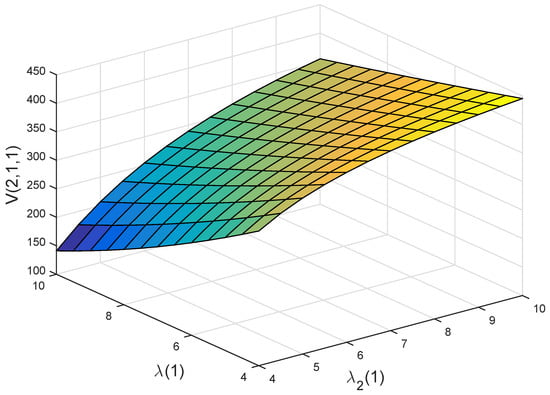
Figure 7.
Joint effects of and on .
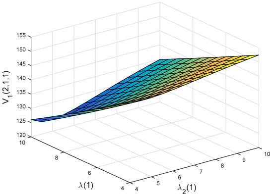
Figure 8.
Joint effects of and on .
Finally, Figure 9 and Figure 10 display the joint effects of and on and , respectively. We find that (resp. ) is increasing with respect to and . These are consistent with what we obtained from Figure 4b,c. More importantly, we find from these two figures that and are more sensitive to than to . This shows that whether a person participates in private health insurance or not, the disposable income has a more significant impact on the policyholder than that of the illness expenditure. The reason is similar to what we have for Figure 5 and Figure 6.
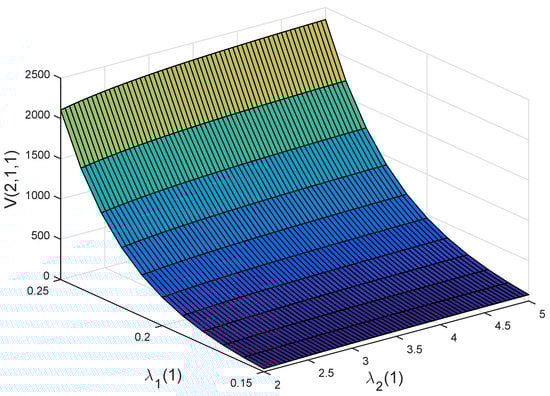
Figure 9.
Joint effects of and on .
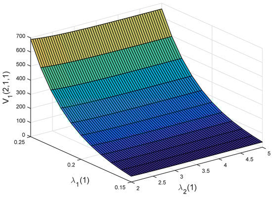
Figure 10.
Joint effects of and on .
Further analysing Figure 5, Figure 6, Figure 7, Figure 8, Figure 9 and Figure 10, we can obtain the following observation: compared with the illness expenditure and the incidence intensity of illness, disposable income has the most significant influence on the policyholder’s decision. This is because the disposable income directly determines whether people buy private health insurance or not and is consistent with the actual situation.
8. Discussion and Conclusions
This article investigated the optimal private health insurance contract design problem, i.e., a game problem with the optimal private health insurance premium. In the game problem, the insurer is the leader and the policyholder is the follower, and they jointly determine the premium. They aim to find the optimal time-consistent strategies that maximize their respective expected terminal wealth and minimize the variance of their terminal wealth. We tackle it under the Nash equilibrium game framework, obtain the optimal time-consistent private health insurance strategies, and finally, determine an optimal private health insurance contract. The theoretical results are illustrated through numerical experiments and some useful observations are derived.
The main findings of this paper include:
- (i)
- The insurer and the policyholder are more sensitive to the other’s risk aversion degree.
- (ii)
- The worse the policyholder’s health, the higher the premium they pay for private health insurance.
- (iii)
- Buying private health insurance can effectively reduce the policyholder’s economic losses caused by illnesses.
- (iv)
- Disposable income has the most significant influence on the policyholder’s decision.
During the determination of the private health premium, the policyholder and the insurer are competitive. For the insurer, the higher the premium, the better, whereas for the policyholder, the lower the premium, the better. Quantifying the competition between the policyholder and the insurer is then quite important. Compared to the experimental method in health sector, the numerical simulation can bring several advantages such as convenient implementation and lower cost. For these reasons and the fact that this paper mainly focuses on theoretical research, in the numerical experiment, some data from the literature and simulation data are adopted. Hence, the numerical result obtained in this paper provides a prediction and may be not accurate. For some related real case studies, please refer to [36,37,38]. On the other hand, it may be better to use the experimental method in the health sector when conducting numerical experiments. For research on the experimental method in the health sector, please refer to [39,40,41]. We will investigate these interesting topics in the future.
Author Contributions
Methodology, P.Y.; investigation, P.Y.; writing—original draft preparation, P.Y.; writing—review and editing, Z.C.; supervision, Z.C.; project administration, Z.C.; funding acquisition, Z.C. and P.Y. All authors have read and agreed to the published version of the manuscript.
Funding
The research was supported by the Natural Science Basic Research Program of Shaanxi of China (Program No. 2023-JC-YB-002), the Humanities and Social Sciences Project of the Ministry of Education of China (Grant No. 21XJC910001), and the National Natural Science Foundation of China (Grant No. 11991023, 11991020).
Institutional Review Board Statement
Not applicable.
Informed Consent Statement
Not applicable.
Data Availability Statement
Not applicable.
Conflicts of Interest
The authors declare no conflict of interest.
References
- Thönnes, S. Ex-post moral hazard in the health insurance market: Empirical evidence from German data. Eur. J. Health Econ. 2019, 20, 1317–1333. [Google Scholar] [CrossRef] [PubMed]
- Artabe, A.; Sigüenza, W. The effects of the economic recession on spending on private health insurance in Spain. Int. J. Health Econ. Manag. 2019, 19, 155–191. [Google Scholar] [CrossRef] [PubMed]
- Nghiem, S.; Graves, N. Selection bias and moral hazard in the Australian private health insurance market: Evidence from the Queensland skin cancer database. Econ. Anal. Policy 2019, 64, 259–265. [Google Scholar] [CrossRef]
- Lapidus, J. Indirect and invisible regulations set in stone: A driving force behind the rise of private health insurance in Sweden. Ann. Am. Acad. Polit. Soc. Sci. 2020, 691, 243–257. [Google Scholar] [CrossRef]
- Menezes, F.N.; Politi, R. Estimating the causal effects of private health insurance in Brazil: Evidence from a regression kink design. Soc. Sci. Med. 2020, 264, 113258. [Google Scholar] [CrossRef]
- Kapur, K. Private health insurance in Ireland: Trends and determinants. Econ. Soc. Rev. 2020, 51, 63–92. [Google Scholar]
- Jamari, J.; Ammarullah, M.I.; Saad, A.P.M.; Syahrom, A.; Uddin, M.; van der Heide, E.; Basri, H. The effect of bottom profile dimples on the femoral head on wear in metal-on-metal total hip arthroplasty. J. Funct. Biomater. 2021, 12, 38. [Google Scholar] [CrossRef]
- Jamari, J.; Ammarullah, M.I.; Santoso, G.; Sugiharto, S.; Supriyono, T.; Permana, M.S.; Winarni, T.I.; van der Heide, E. Adopted walking condition for computational simulation approach on bearing of hip joint prosthesis: Review over the past 30 years. Heliyon 2022, 8, e12050. [Google Scholar] [CrossRef]
- Prakoso, A.T.; Basri, H.; Adanta, D.; Yani, I.; Ammarullah, M.I.; Akbar, I.; Ghazali, F.A.; Syahrom, A.; Kamarul, T. The effect of tortuosity on permeability of porous scaffold. Biomedicines 2023, 11, 427. [Google Scholar] [CrossRef]
- Blomqvist, Å. Optimal non-linear health insurance. J. Health Econ. 1997, 16, 303–321. [Google Scholar] [CrossRef]
- Ma, C.-T.A.; McGuire, T.G. Optimal health insurance and provider payment. Am. Econ. Rev. 1997, 87, 685–704. [Google Scholar]
- Cutler, D.M.; Zeckhauser, R.J. The anatomy of health insurance. Handbook Health Econ. 2000, 1, 563–643. [Google Scholar]
- Migon, H.S.; Moura, F.A.S. Hierarchical Bayesian collective risk model: An application to health insurance. Insur. Math. Econ. 2005, 36, 119–135. [Google Scholar] [CrossRef]
- Baione, F.; Levantesi, S. A health insurance pricing model based on prevalence rates: Application to critical illness insurance. Insur. Math. Econ. 2014, 58, 174–184. [Google Scholar] [CrossRef]
- Dhaene, J.; Hanbali, H. Measuring medical infation for health insurance portfolios in Belgium. Eur. Actuar. J. 2019, 9, 139–153. [Google Scholar] [CrossRef]
- Hambel, C. Health shock risk, critical illness insurance, and housing services. Insur. Math. Econ. 2020, 91, 111–128. [Google Scholar] [CrossRef]
- Martinon, P.; Picard, P.; Raj, A. On the design of optimal health insurance contracts under ex post moral hazard. Geneva Risk Insur. Rev. 2018, 43, 137–185. [Google Scholar] [CrossRef]
- Golubin, A.Y. Pareto-optimal insurance policies in the models with a premium based on the actuarial value. J. Risk Insur. 2006, 73, 469–487. [Google Scholar] [CrossRef]
- Ahmad, N.; Aggarwal, K. Health shock, catastrophic expenditure and its consequences on welfare of the household engaged in informal sector. J. Public Health 2017, 25, 611–624. [Google Scholar] [CrossRef]
- Ma, X.; Wang, Z.; Liu, X. Progress on catastrophic health expenditure in China: Evidence from China family panel studies (CFPS) 2010 to 2016. Int. J. Environ. Res. Public Health 2019, 16, 4775. [Google Scholar] [CrossRef]
- Zhu, D.; Shi, X.; Nicholas, S. Estimated annual prevalence, medical service utilization and direct costs of lung cancer in urban China. Cancer Med. 2021, 10, 2914–2923. [Google Scholar] [CrossRef] [PubMed]
- Yang, P.; Chen, Z. Optimal time-consistent social health insurance and private health insurance strategy under a new health insurance framework. Appl. Stoch. Model. Bus. 2022, 38, 726–743. [Google Scholar] [CrossRef]
- Karatzas, I.; Shreve, S.E. Brownian Motion and Stochastic Calculus; Springer: New York, NY, USA, 1991. [Google Scholar]
- Bensoussan, A.; Siu, C.C.; Yam, S.C.P.; Yang, H. A class of non-zero-sum stochastic differential investment and reinsurance games. Automatica 2014, 50, 2025–2037. [Google Scholar] [CrossRef]
- Yao, H.; Yang, Z.; Chen, P. Markowitz’s mean-variance defined contribution pension fund management under inflation: A continuous-time model. Insur. Math. Econ. 2013, 53, 851–863. [Google Scholar] [CrossRef]
- Brachetta, M.; Ceci, C. Optimal proportional reinsurance and investment for stochastic factor models. Insur. Math. Econ. 2019, 87, 15–33. [Google Scholar] [CrossRef]
- Chen, Z.; Yang, P. Robust optimal reinsurance-investment strategy with price jumps and correlated claims. Insur. Math. Econ. 2020, 92, 27–46. [Google Scholar] [CrossRef]
- Yang, P.; Chen, Z.; Cui, X. Equilibrium reinsurance strategies for n insurers under a unified competition and cooperation framework. Scand. Actuar. J. 2021, 2021, 969–997. [Google Scholar] [CrossRef]
- Björk, T.; Murgoci, A.; Zhou, X.Y. Mean-variance portfolio optimization with state-dependent risk aversion. Math. Financ. 2014, 24, 1–24. [Google Scholar] [CrossRef]
- Yang, P.; Chen, Z.; Wang, L. Time-consistent reinsurance and investment strategy combining quota-share and excess of loss for mean-variance insurers with jump-diffusion price process. Commun. Stat.-Theory Methods 2021, 50, 2546–2568. [Google Scholar] [CrossRef]
- Klodeen, P.E.; Platen, E. Numerical Solution of Stochastic Differential Equation; Springer: Berlin/Heidelberg, Germany, 1995. [Google Scholar]
- Zhang, C.; Liang, Z.; Yuen, K.C. Optimal reinsurance and investment in a Markovian regime-switching economy with delay and common shock. Sci. Sin. Math. 2021, 51, 773–796. (In Chinese) [Google Scholar]
- Chen, L.; Shen, Y. On a new paradigm of optimal reinsurance: A stochastic stackelberg differential game between an insurer and a reinsurer. ASTIN Bull. 2018, 48, 905–960. [Google Scholar] [CrossRef]
- Chen, L.; Shen, Y. Stochastic Stackelberg differential reinsurance games under time-inconsistent mean-variance framework. Insur. Math. Econ. 2018, 88, 120–137. [Google Scholar] [CrossRef]
- Yang, P.; Chen, Z. Optimal reinsurance pricing, risk sharing and investment strategies in a joint reinsurer-insurer framework. IMA J. Manag. Math. 2022, dpac002. [Google Scholar] [CrossRef]
- Tauviqirrahman, M.; Ammarullah, M.I.; Jamari, J.; Saputra, E.; Winarni, T.I.; Kurniawan, F.D.; Shiddiq, S.A.; van der Heide, E. Analysis of contact pressure in a 3D model of dual-mobility hip joint prosthesis under a gait cycle. Sci. Rep. 2023, 13, 3564. [Google Scholar] [CrossRef] [PubMed]
- Jamari, J.; Ammarullah, M.I.; Santoso, G.; Sugiharto, S.; Supriyono, T.; van der Heide, E. In silico contact pressure of metal-on-metal total hip implant with different materials subjected to gait loading. Metals 2022, 12, 1241. [Google Scholar] [CrossRef]
- Jamari, J.; Ammarullah, M.I.; Santoso, G.; Sugiharto, S.; Supriyono, T.; Prakoso, A.T.; Basri, H.; van der Heide, E. Computational contact pressure prediction of CoCrMo, SS 316L and Ti6Al4V femoral head against UHMWPE acetabular cup under gait cycle. J. Funct. Biomater. 2022, 13, 64. [Google Scholar] [CrossRef]
- Ammarullah, M.I.; Afif, I.Y.; Maula, M.I.; Winarni, T.I.; Tauviqirrahman, M.; Akbar, I.; Basri, H.; van der Heide, E.; Jamari, J. Tresca stress simulation of metal-on-metal total hip arthroplasty during normal walking activity. Materials 2021, 14, 7554. [Google Scholar] [CrossRef]
- Ammarullah, M.I.; Santoso, G.; Sugiharto, S.; Supriyono, T.; Wibowo, D.B.; Kurdi, O.; Tauviqirrahman, M.; Jamari, J. Minimizing risk of failure from ceramic-on-ceramic total hip prosthesis by selecting ceramic materials based on tresca stress. Sustainability 2022, 14, 13413. [Google Scholar] [CrossRef]
- Ammarullah, M.I.; Hartono, R.; Supriyono, T.; Santoso, G.; Sugiharto, S.; Permana, M.S. Polycrystalline diamond as a potential material for the hard-on-hard bearing of total hip prosthesis: Von mises stress analysis. Biomedicines 2023, 11, 951. [Google Scholar] [CrossRef]
Disclaimer/Publisher’s Note: The statements, opinions and data contained in all publications are solely those of the individual author(s) and contributor(s) and not of MDPI and/or the editor(s). MDPI and/or the editor(s) disclaim responsibility for any injury to people or property resulting from any ideas, methods, instructions or products referred to in the content. |
© 2023 by the authors. Licensee MDPI, Basel, Switzerland. This article is an open access article distributed under the terms and conditions of the Creative Commons Attribution (CC BY) license (https://creativecommons.org/licenses/by/4.0/).