1. Introduction
The debts coming from clients with unpaid credits have an important impact in the solvency of banks and other credit institutions. According to the Basel Committee on Banking Supervision of the Bank for International Settlements, one of the crucial elements for the risk measurement of capital assignments is the probability of default. For a fixed time,
t, and a horizon time,
b, the probability of default (PD) can be defined as the probability that a credit that has been paid until time
t becomes unpaid not later than time
. The PD is allowed to depend on the credit scoring
x, which is, usually, some linear combination of informative covariates of the credit and the clients. Standard methods to estimate the PD include logistic models and other binary response parametric regression models. See the studies of [
1,
2,
3,
4,
5,
6], among others.
In recent years, survival analysis has started to be considered an interesting tool in credit risk problems. Since the work by [
7], some literature has been developed following this line. See the works of [
8,
9,
10,
11,
12,
13,
14]. Nonparametric estimators of the probability of default based on conditional survival function estimators are presented in [
12,
13] since the probability of default can be written in terms of the conditional survival function in a right censored context. All these nonparametric estimators are based on covariate smoothing. In the recent work [
14], a general nonparametric estimator of the probability of default with double smoothing, both in the covariate and in the time variable, was proposed and studied.
In particular, Beran’s estimator and a doubly smoothed Beran’s estimator of the PD were presented in [
13,
14], respectively, and their asymptotic properties were analyzed. Simulation studies carried out in these papers show a good performance of the estimators, especially of the doubly smoothed Beran’s estimator. However, these previous studies were carried out using theoretical smoothing parameters. Since the integrated mean square error expressions are complex and depend on several population parameters, they are not useful in practice to obtain plug-in estimations of these theoretical bandwidths. The goal of this work is to propose resampling techniques to approximate them.
Bootstrap has become a strong tool in many statistical applications since it was first introduced by [
15]. Bootstrap for right censored data was first proposed by [
16] and the bootstrap method and its applications were studied in [
17]. Asymptotic theory of bootstrap for right censored data was stablished by [
18,
19]. In [
20], bootstrap for nonparametric regression with right censored observations at fixed covariate values was studied. A bootstrap approach for the nonparametric censored regression setup was studied in [
21]. In [
22] a local cross-validation bandwidth selector was proposed.
Our approach follows the ideas of [
21], and it is based on the obvious bootstrap. Both Beran and smoothed Beran’s estimators are bootstrapped in order to approximate their corresponding optimal bandwidths. The bootstrap is also useful to compute confidence regions, as the existing theoretical result only allows to compute pointwise and theoretical confidence intervals, which are not computable in practice since the variance of the estimator again depends on unknown population quantities. A bootstrap algorithm to compute confidence regions for the probability of default is also proposed.
The remainder of this paper is organized as follows. In
Section 2, bootstrap selectors for the bandwidths of Beran and smoothed Beran’s estimators are proposed. In
Section 3, a simulation study shows the behavior of the PD estimators with bootstrap bandwidths. The issue of obtaining confidence regions for the probability of default,
, for a fixed value of
and
t covering the interval
is addressed in
Section 4 using Beran and smoothed Beran’s estimators. A simulation study on the proposed methods for computing confidence regions is shown in
Section 5. In
Section 6, Beran’s estimator and the smoothed Beran’s estimator with bootstrap bandwidths are used to estimate the probability of default function conditional on the credit scoring for a German credit dataset.
Section 7 contains some concluding remarks.
2. Bandwidth Selection for Beran and Smoothed Beran’s PD Estimators
Consider the right censored simple random sample of where represents the covariate, the observed lifetime and the censoring indicator, where and are the time to occurrence of the event and the censoring time for the i-th individual of the sample with . In credit risk, usually, X is the credit scoring, Z is the observed maturity, T is the time to default, and C is the time until the end of the study or the anticipated cancellation of the credit. The distribution function of T is denoted by and the survival function by . The functions and are the conditional distribution and survival functions of T evaluated at t given . The conditional distribution function of Z is denoted by , and the conditional distribution function of C is denoted by . It is assumed that an unknown relationship between T and X exists. Given , the distributions of T and C conditional to are supposed to be independent.
Let
be a fixed value of the covariate
X and
a fixed positive time. Then, the probability of default in a time horizon
from a maturity time,
t, is defined as follows:
In this section, methods for the automatic selection of the bandwidths for Beran’s estimator and the smoothed Beran’s estimator of the probability of default are proposed.
2.1. Beran’s Estimator
Beran’s estimator of the conditional survival function is given by
where
with
,
is a kernel function and
is the bandwidth that determines the smoothness introduced in the estimator through the covariate
X.
Plugging (
2) into (
1), the probability of default estimator based on Beran’s PD estimator is obtained:
In this section, bootstrap methods are proposed for the automatic selection of
h. There are two classic methods for bootstrap resampling in a censoring context: the obvious bootstrap and the simple bootstrap. The equivalence between both methods in an unconditional setup is proved in [
16]. In [
21], this result is extended to the case where a covariate is involved, assuming there is no ties in the sample values of the covariate. This was done by proving the equivalence of the two resampling methods, the obvious bootstrap and the simple weighted bootstrap. In this paper, the following obvious bootstrap method combined with a smoothed bootstrap for the covariate is proposed.
2.1.1. Algorithm for Bootstrap Resampling
Let be an interval containing appropriate bandwidth values and let be the pilot bandwidth for the bootstrap resampling:
Obtain iid with and iid with common density K for all .
For each
, define
where
is the integer part of
u. Generate
from Beran’s estimator of the conditional distribution of
T using the sample
and bandwidth
r, denoted by
, and
from the Beran’s estimator of the conditional distribution of
C using the sample
and bandwidth
r, denoted by
.
The estimators and are forced to be equal to one from the last observed lifetime () onwards.
For each
, obtain
Consider the bootstrap resample .
In this paper, we want to estimate the probability of default function,
, for a fixed
and
t covering the interval
. Therefore, our goal is to get the bandwidth
that minimizes the mean integrated squared error given by
whose bootstrap approximation is
where
is the estimation of the theoretical PD with pilot bandwidth
r, using the sample
and
is the bootstrap estimation of
with bandwidth
h, using the bootstrap resample
.
The resampling distribution of
cannot be computed in a close form, so the Monte Carlo method is used. It is based on obtaining
B bootstrap resamples and estimating
for each of them. Thus, the distribution of
is approximated by the empirical one of
, obtained from
B bootstrap resamples and the bootstrap version of the estimation error committed by Beran’s estimator for any smoothing parameter
h is given by
Likewise, the integral is approximated by a Riemann sum.
2.1.2. Algorithm for Bootstrap Bandwidth Selector Based on Beran’s Estimator
Let be a fixed value of the covariate, and :
Compute from the original sample .
Obtain B bootstrap resamples of the form with using the smoothed bootstrap with pilot bandwidth and calculate for each of them.
Approximate
according to (
5).
Repeat Steps 1–3 for values of h in a grid of .
Select the value of h that provides the smallest as the bootstrap bandwidth .
Concerning the auxiliary bandwidth
, a preliminary analysis not shown here suggests
where
is the
u quantile of the sample
, as a suitable pilot bandwidth in this context.
Note that the proposed algorithm is also valid to obtain a bootstrap approximation of the optimal bandwidth for the estimation of
for fixed values of
and
by replacing
by
, which is the bootstrap analogue of
2.2. Smoothed Beran’s Estimator
Nonparametric estimators for the probability of default such as Beran’s estimator,
, are smoothed in the covariate
X. It is interesting to consider estimators with double smoothing both in the covariate,
X, and in the time variable,
T. This idea was previously used in [
23,
24,
25] to obtain doubly smoothed estimators of the conditional survival function. In [
14], a doubly smoothed version of PD Beran’s estimator was proposed based on a further smoothing, in time, of Beran’s estimator of the conditional survival function ([
26]). Asymptotic properties and simulation studies carried out in [
14] show that the doubly smoothed Beran’s estimator performs better than the classical Beran’s estimator when estimating the probability of the default curve. This section presents a method for automatic selection of the bandwidths on which it depends.
Let
be Beran’s estimator of the conditional survival function given in (
2) with
being the smoothing parameter for the covariate. Then, the expression for the doubly smoothed Beran’s estimator of the conditional survival function defined in [
25] is as follows:
with
where
is the
i-th element of the sorted sample of
Z,
is the distribution function of a kernel
K,
, and
is the smoothing parameter for the time variable. Then, plugging (
7) into (
1), the probability of the default estimator based on the smoothed Beran’s survival estimator is obtained:
A bootstrap method is proposed for the automatic selection of the bivariate bandwidth .
2.2.1. Algorithm for Bootstrap Resampling
Let and be intervals containing appropriate bandwidth values and let and be pilot bandwidths for the smoothed resample of X, T and C:
Obtain iid with and iid with common density K, iid with common density K and iid with common density K for all .
For each
, obtain
where
is resampled from
constructed using Beran’s estimator with the sample
and
is resampled from
constructed using Beran’s estimator with the sample
.
For each
, obtain
Consider the bootstrap resample .
The conditional distribution functions of and are, respectively, the smoothed Beran’s estimators and .
The optimal bivariate bandwidth,
is defined as the pair of bandwidths that minimizes the mean integrated squared error given by
The bootstrap version of
is given by
where
is the smoothed Beran’s PD estimation with pilot bandwidths
using the sample
and
is the bootstrap estimation of
with bandwidths
, using the bootstrap resample
. Since the sampling distribution of
is unknown, the Monte Carlo method gives the following approximation
based on the empirical distribution of
obtained from
B bootstrap resamples. The integral is approximated by a Riemann sum.
2.2.2. Algorithm for Bootstrap Bandwidth Selector Based on the Smoothed Beran’s Estimator
Let x be a fixed value of the covariate, and :
Compute from the original sample .
Obtain B bootstrap resamples of the form with using the doubly smoothed bootstrap and calculate for each of them.
Approximate
according to (
10).
Repeat Steps 1–3 for pairs of values in a grid of .
Obtain the pair that provides the smallest as the bootstrap bandwidth .
The auxiliary bandwidth
was defined in (
6). The pilot bandwidth
for the time variable smoothing is
where
is the
u quantile of the sample
.
3. Simulation Study for Bandwidth Selection
A simulation study was conducted in order to show the behavior of bootstrap bandwidth selectors for Beran’s and smoothed Beran’s estimators proposed in
Section 2. Two models are considered, one with Weibull lifetime and censoring time distributions and another one with exponential distributions.
Model 1 considers a
distribution for
X. The time to occurrence of the event conditional to the covariate,
, follows a Weibull distribution with parameters
and
where
, and the censoring time conditional to the covariate,
, follows a Weibull distribution with parameters
and
where
. In this case, the conditional survival function and the censoring conditional probability are given by
Having set the value of the covariate , the value of is chosen so that the censoring conditional probability is and . These values are and , respectively. The conditional survival function for this model is estimated in a time grid of size , , where and , i.e., about of the time grid range for the value of the covariate . Therefore, in this case, .
Model 2 also considers a
distribution for
X. The time to occurrence of the event conditional to the covariate,
, follows an exponential distribution with parameter
, and the censoring time conditional to the covariate,
, follows an exponential distribution with parameter
. In this scenario, the conditional survival function and the censoring conditional probability are the following:
Having set the value of the covariate, , the value of is chosen so that the censoring conditional probability is and . These values are and , respectively. The conditional survival function is estimated in a time grid of size , , where and , i.e., about of the time grid range for the value of the covariate . Therefore, in this case, .
It can be proved that Model 1 is close to a proportional hazards model, while Model 2 moves away from this parametric model. These two models were used in the simulation study carried out by [
14].
The boundary effect is corrected using the reflexion principle, and the truncated Gaussian kernel with a truncation range
is considered. The size of the lifetime grid is
. The sample size is
. The simulation study is carried out with software developed in R by the authors themselves. In order to minimize the
MISE error function without increasing CPU time more than necessary, a limited-memory algorithm for solving large nonlinear optimization problems is used, L-BFGS-B. It was proposed by [
27] for solving optimization problems subject to simple bounds on the variables in which information on the Hessian matrix is difficult to obtain. Results of numerical studies about this method are shown in [
27]. It is available at the stats package from the Comprehensive R Archive Network (CRAN) using Fortran 77 subroutines (see [
28]).
3.1. Simulation Study for Beran’s Estimator
In this subsection, the behavior of the bootstrap bandwidth selector for Beran’s estimator is shown. For each model, the estimation error function is approximated via Monte Carlo using 300 simulated samples. The bandwidth that minimises is obtained and denoted by . The values of and are used as a benchmark.
In the simulation study,
simulated samples are used. For each sample,
bootstrap resamples are obtained to approximate the bootstrap
MISE function,
, and obtain the bootstrap bandwidth associated to each simulated sample
,
. The mean value of the
N bootstrap bandwidths and the standard deviation are defined as follows
As a relative measure of the difference between the bootstrap bandwidth and the optimal one, we compute
with
. The mean of the absolute value of these relative deviations,
, is a good measure of how close the bootstrap bandwidth is to the optimal one.
For each sample, the estimation error committed by Beran’s estimator with the corresponding bootstrap bandwidth,
and its squared root,
, are approximated via Monte Carlo using 300 simulated samples. The mean of these estimation errors given by
is used as a measure of the estimation error made by the bootstrap bandwidth, when compared with the estimation error made by the
MISE bandwidth.
As a relative measure of the difference between the estimation errors using the bootstrap and the
MISE bandwidths, the following ratios are defined:
satisfying
for all
. The mean of the
values with
is denoted by
. Small values (close to zero) of
and
indicate good behavior of the bootstrap bandwidth. Values of the bootstrap bandwidths, estimation errors and relative measures for Models 1 and 2 are included in
Table 1. The results show a good performance of the proposed bootstrap selector.
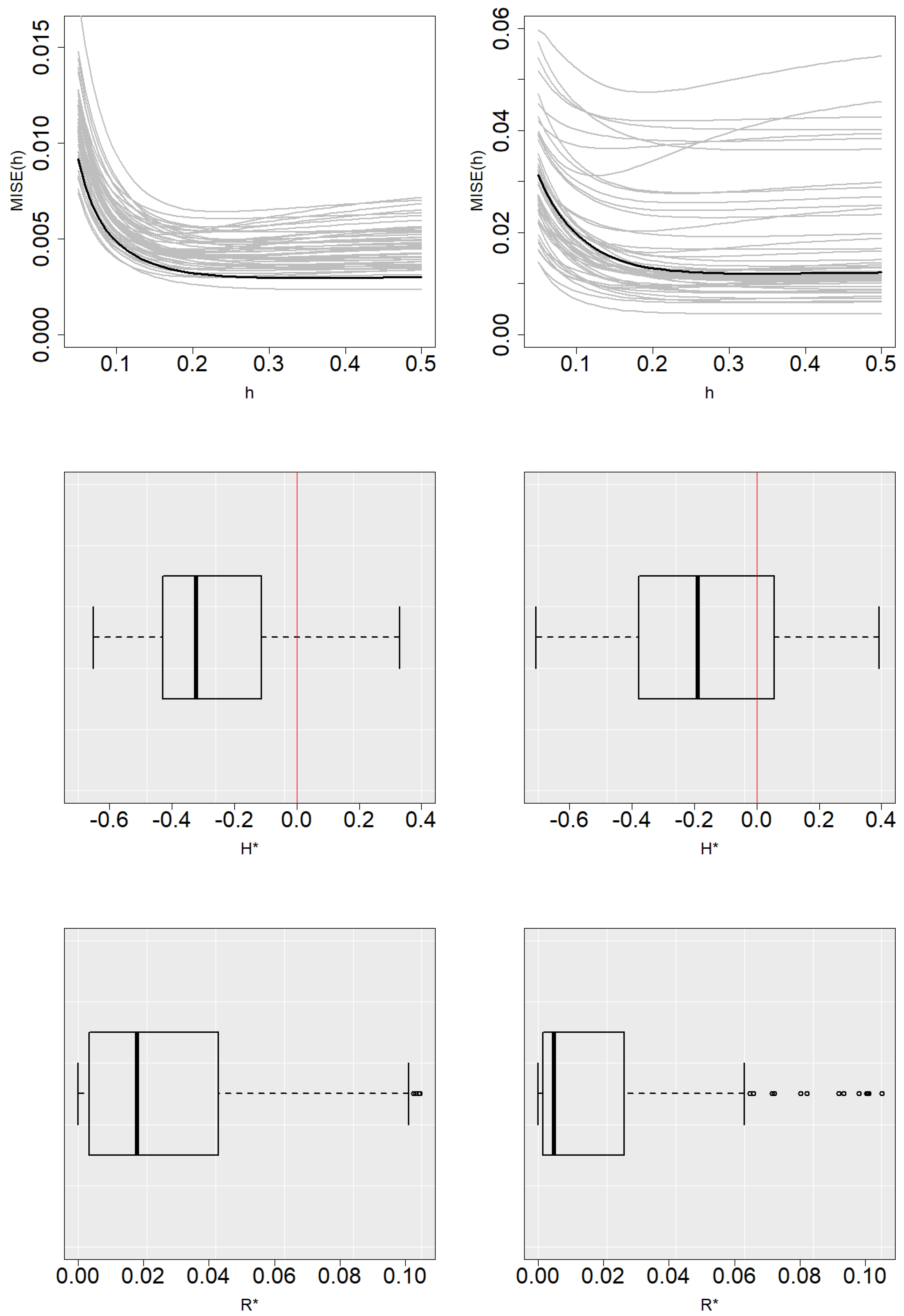
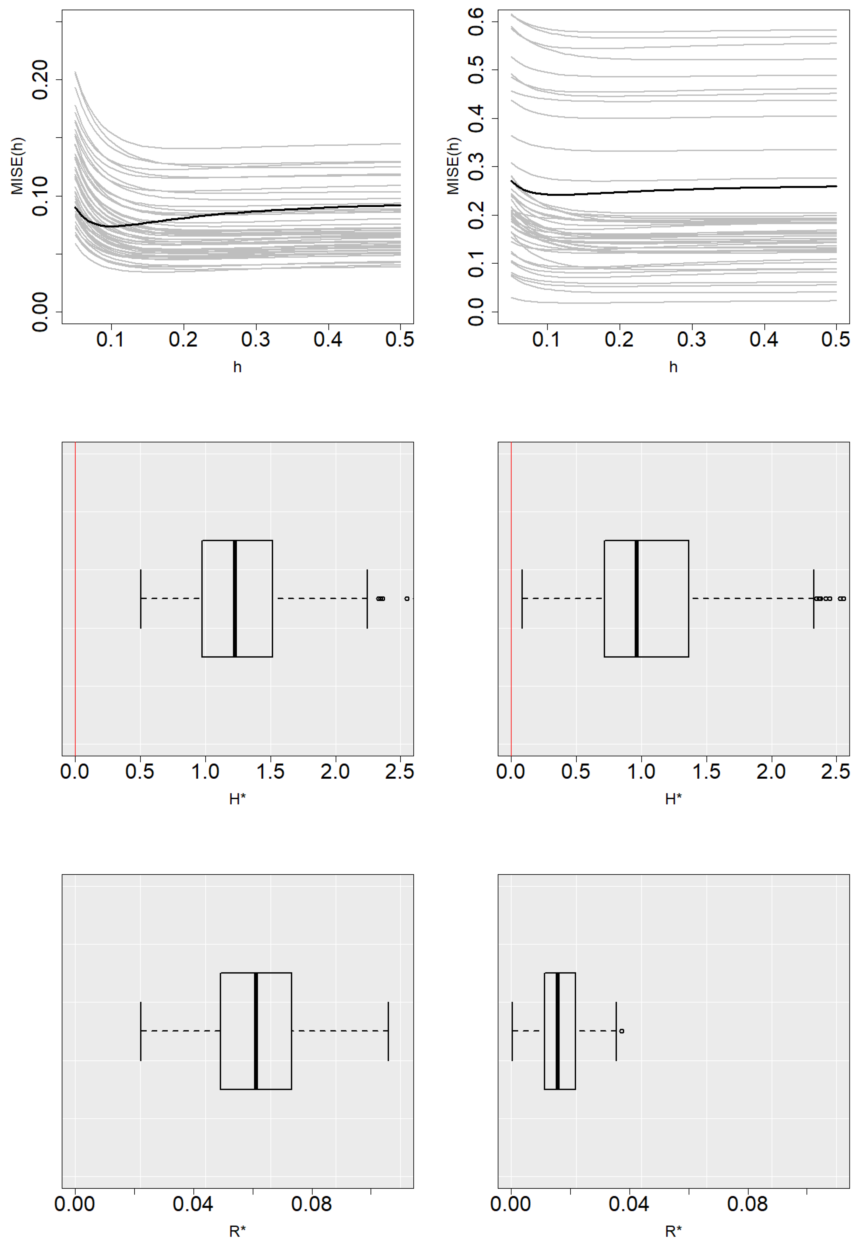
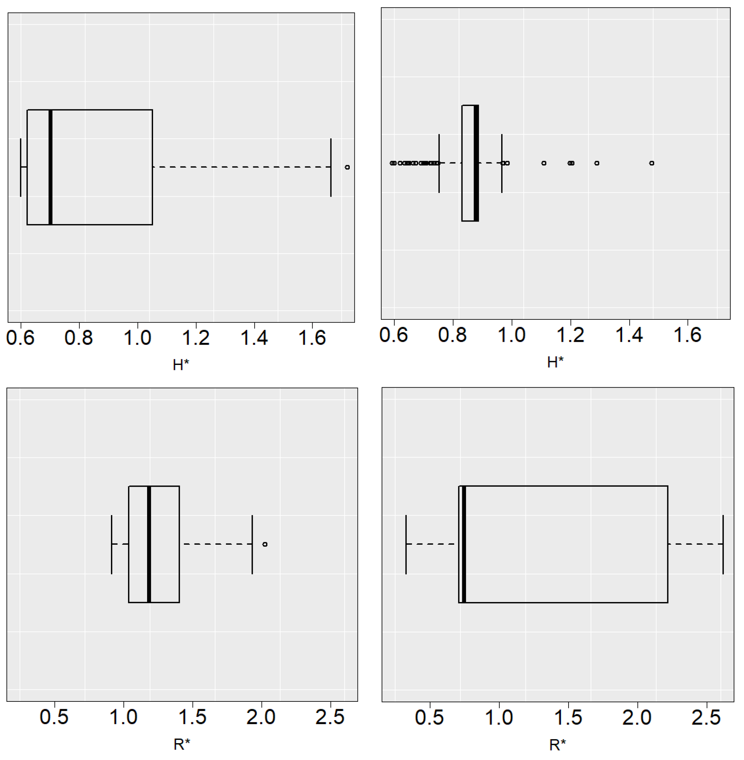
Figure 1 and
Figure 2 show the function
along with the Monte Carlo approximations of
for some simulated samples and the boxplots of
and
with
for Models 1 and 2. The method tends to slightly underestimate the value of
with respect to
in Model 1 and overestimate its value in Model 2, which is reflected in the boxplots of
. Nevertheless, these figures show that the
curve is fairly flat and variations in the selection of
h do not imply an important increase in the estimation error.
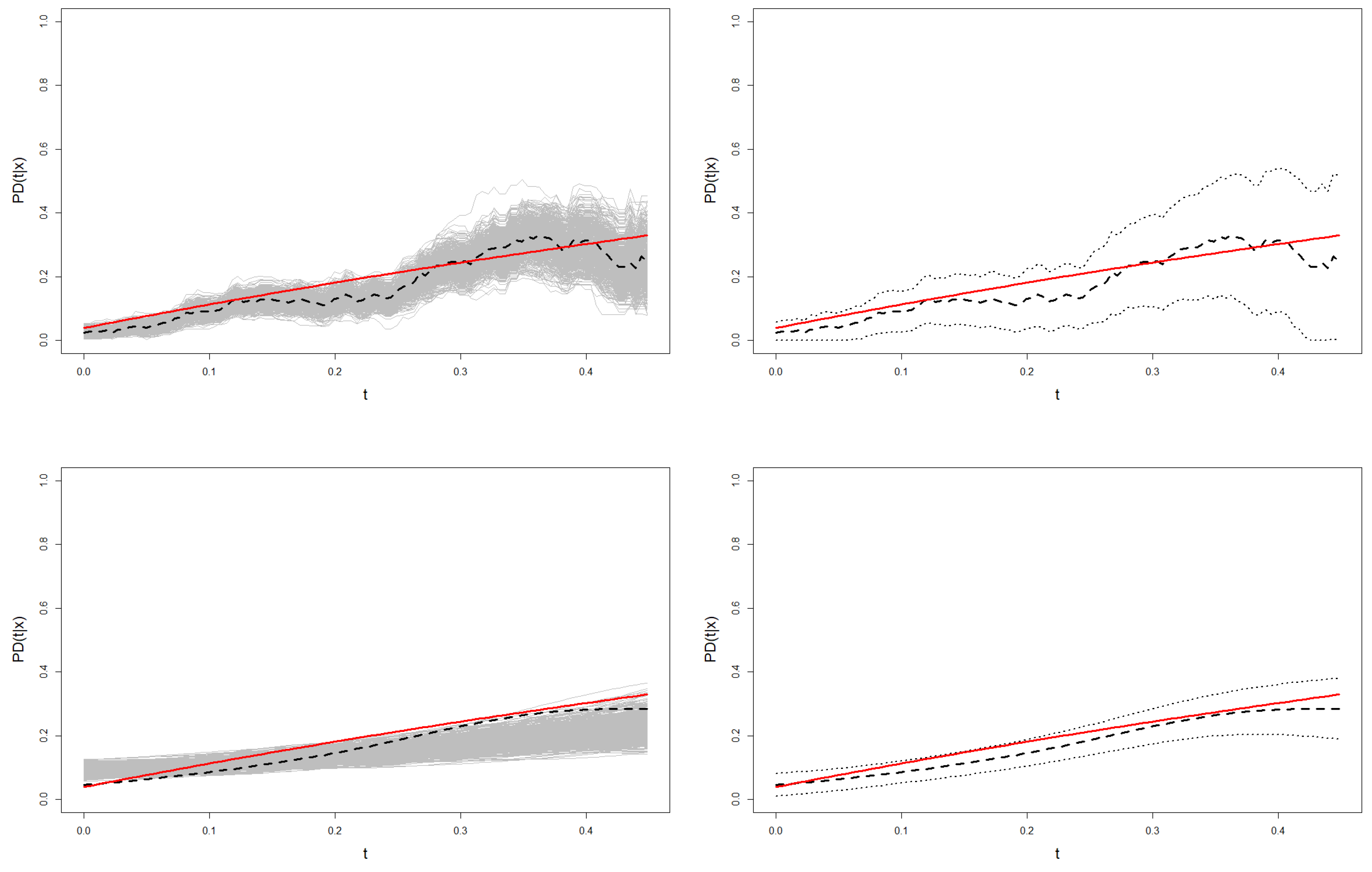
In order to illustrate the results,
Figure 3 shows the theoretical probability of default function and Beran’s estimation with the
MISE and bootstrap bandwidths drawn for one sample from Model 1 and 2 when the conditional probability of censoring is
. For large values of time, the performance of the estimator becomes worse, due to the fact that in that region there are few data, most of them censored, and therefore offering poor information.
3.2. Simulation Study for the Smoothed Beran’s Estimator
In this section, a simulation study on the bootstrap bandwidth selector of the smoothed Beran’s estimator in (
8) is carried out. The resampling technique and Monte Carlo approximation of the
MISE presented in
Section 2.2 are used.
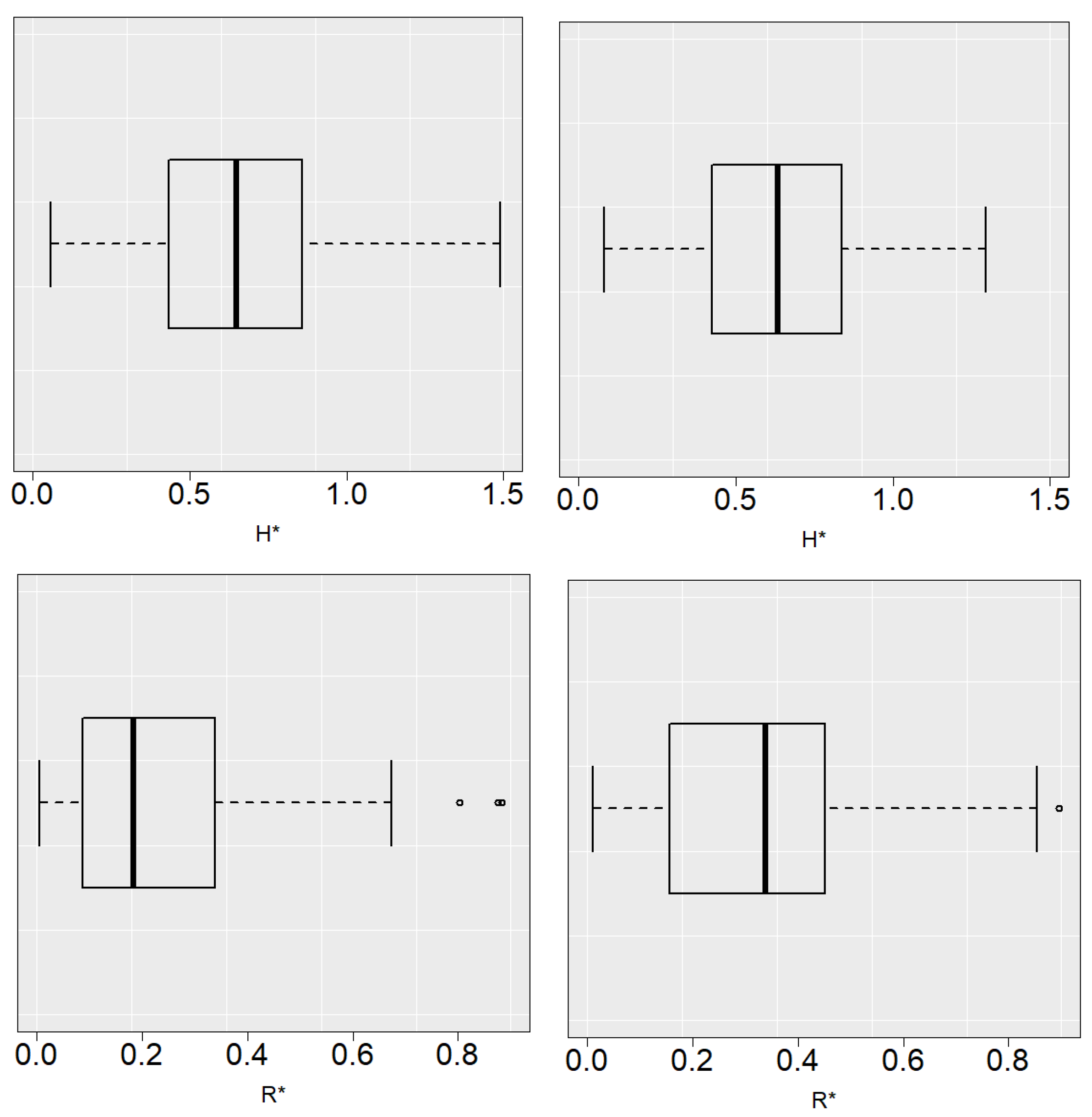
For each model, the error function is approximated via Monte Carlo from 300 simulated samples, and the bivariate bandwidth that minimizes is obtained and denoted by . The values of and are used as a benchmark.
In the study,
samples are simulated. For each simulated sample, the corresponding bootstrap bandwidths are approximated from
resamples, obtaining
with
. The mean value of the
N bootstrap bandwidths and the standard deviation are the following:
In order to measure the distance of the bootstrap bidimensional bandwidth of the
j-th sample,
, from the corresponding
MISE bandwidth,
, consider the vector
and its Euclidean norm denoted by
with
. The mean value,
is a measure of how close the bootstrap bandwidths are to the
MISE one.
For each sample, the estimation error committed by the smoothed Beran’s estimator with the corresponding bootstrap bandwidth,
and its squared root,
, are approximated via Monte Carlo using 300 simulated samples. The mean of these estimation errors given by
is used as a measure of the estimation error committed by the bootstrap bidimensional bandwidth in the model.
The ratio
is defined as a relative measure of the difference between the error committed by the estimator with bootstrap bandwidth and
MISE bandwidth. The mean of the positive values
with
is denoted by
. Values of the bootstrap bivariate bandwidths, estimation errors and relative measures for Models 1 and 2 are included in
Table 2.
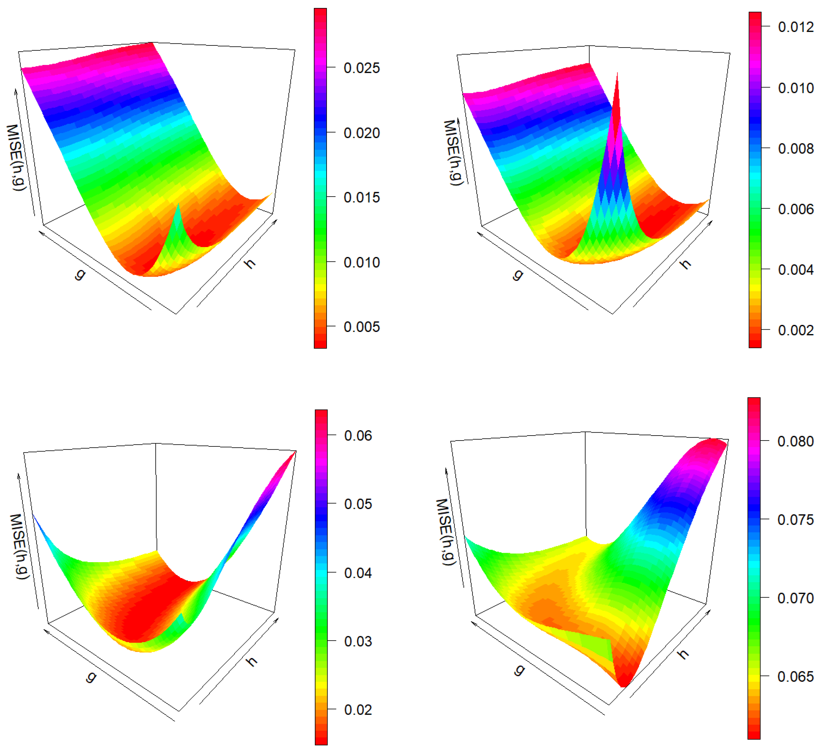
Figure 4 shows the
function of the smoothed Beran’s estimator and its bootstrap approximation for one sample of both Models 1 and 2 when the conditional probability of censoring is
. It is approximated on a grid of 50 values of
h and 50 values of
g. Note that both
and
curves for each fixed
h value are quite similar in the region close to the minimum value of
. Thus, the influence of covariate smoothing parameter
h is weak when estimating the PD using values of bandwidth
g close to the optimal one.
Figure 5 and
Figure 6 show the boxplots of
and
with
. In general, the selector tends to underestimate the value of the bandwidths. Due to the behavior of the
curves mentioned above, this does not lead to a significant increase in the estimation error.
Figure 7 shows the theoretical probability of the default function and Beran’s estimation with
MISE and bootstrap bandwidths for one sample from Models 1 and 2 when the conditional probability of censoring is
. Comparing this figure with the equivalent one for Beran’s estimator shown in
Figure 3, the improvement in estimation due to the double smoothing is remarkable.
The results showed in
Table 1 and
Table 2 are summarized in
Table 3 to compare the behavior of Beran (BERAN) and the smoothed Beran’s (SBERAN) estimators for the PD and to evaluate whether the improvement that smoothing in the time variable provides for PD estimation is preserved when approximating the smoothing parameters by resampling techniques.
Table 3 shows the estimation errors committed by Beran and the smoothed Beran’s estimators of the probability of default using bootstrap bandwidths. In order to measure the increase in estimation error resulting from using Beran’s estimator, the following ratio is defined:
and included in
Table 3.
In Model 1, the estimation error committed by Beran’s estimator is larger than the error committed by the smoothed Beran’s estimator when the conditional probability of censoring is 0.2 and by when the conditional probability of censoring is 0.5. In Model 2, these differences are even more significant: the estimation error increases up to when using Beran’s estimator with bootstrap bandwidth instead of the doubly smoothed Beran’s estimator.
4. Confidence Regions Using Beran and Smoothed Beran’s Estimators
Let
be a fixed value of the covariate and consider
the probability of default curve with
. The curve
belongs to the function space
whose elements are real-valued functions with domain
. From the sample
, Beran’s estimation of
,
, is obtained and a confidence region of
at
confidence level associated to Beran’s estimator can be constructed. A similar construction is done for the smoothed Beran’s estimator. This confidence region of
is a random subset of
denoted by
that satisfies
In this section, a method for constructing confidence regions, , based on Beran and the smoothed Beran’s estimator is developed.
First, Beran’s estimator of the probability of default,
, given in (
3) is used. This method follows the ideas of [
29] to obtain prediction regions. It is based on finding the value of
such that
with
. Thus, the theoretical confidence region is defined by
Since
and
are unknown, they are approximated by means of a bootstrap technique. The bootstrap confidence region is defined as follows:
where
is the bootstrap estimation of
with bandwidth
h and
and
are the bootstrap analogue of
and
. The confidence region
satisfies
From the original sample , Beran’s estimator of is obtained with appropriate bandwidth h, . The algorithm to obtain the bootstrap confidence region for at confidence level associated to is explained below. The Monte Carlo method is used to approximate , and an iterative method is used to approximate the value of so that the confidence region has a confidence level approximately equal to .
4.1. Confidence Region Based on Beran’s Estimator
Compute Beran’s estimator from the original sample and pilot bandwidth .
Generate
B bootstrap resamples of the form
by means of the resampling algorithm presented in Sub
Section 2.1 and pilot bandwidth
r.
For , compute with the k-th bootstrap resample and bandwidth h, obtaining .
Approximate the standard deviation of
by
Use an iterative method to obtain an approximation of the value
defined in (
12).
The confidence region is given by
4.2. Iterative Method to Approximate
The iterative method to approximate the value of so that the confidence region has a confidence level approximately equal to is explained below. This algorithm allows the parameter to be approximated quickly and efficiently.
Let
be the Beran’s estimations of the PD with bandwidth
h over a set of
B bootstrap resamples of
. Define the Monte Carlo approximation of
in (
12), for any
, as follows:
Let be such that and let be a tolerance, for example, .
A preliminary analysis not shown here suggests the following pilot bandwidth:
This method to obtain confidence regions for the curve
for fixed
and
t covering
based on Beran’s estimator can be adapted to obtain confidence regions using the doubly smoothed Beran’s estimator. Simply replace Beran’s estimator
by the smoothed Beran’s estimator
given in (
8) where necessary, and obtain the analogous bootstrap approximations of
and
. The confidence region is given by
Denote the lower and upper bounds of the confidence region by and , respectively. It may happen that the lower bound of the confidence region is less than 0 or the upper bound is greater than 1 for some points . When this happens, we set or , as appropriate.
The pilot bandwidths defined in (
6) and (
11) are used for the confidence region algorithm based on both Beran and smoothed Beran’s estimators.
5. Simulation Study for Confidence Regions
A simulation study is carried out to test the performance of bootstrap confidence regions proposed. Models 1 and 2 described in
Section 3 are considered in this study, with identical features. The methods shown in
Section 4 are used for this purpose with both Beran and smoothed Beran’s estimators. When Beran’s estimator is used, the bandwidth that minimizes the mean integrated squared error,
, is used. Similarly, if the smoothed Beran’s estimator is used, the two-dimensional bandwidth that minimizes the mean integrated squared error,
, is used. These bandwidths are unknown in practice, but they allow a fair comparison of methods in the simulation study.
The simulation set-up is the one explained in
Section 3. Two conditional probabilities of censoring are considered for each model:
and
. The number of bootstrap resamples of each samples is
, and
simulated samples of each model are obtained. The sample size is
. The confidence level is
with
.
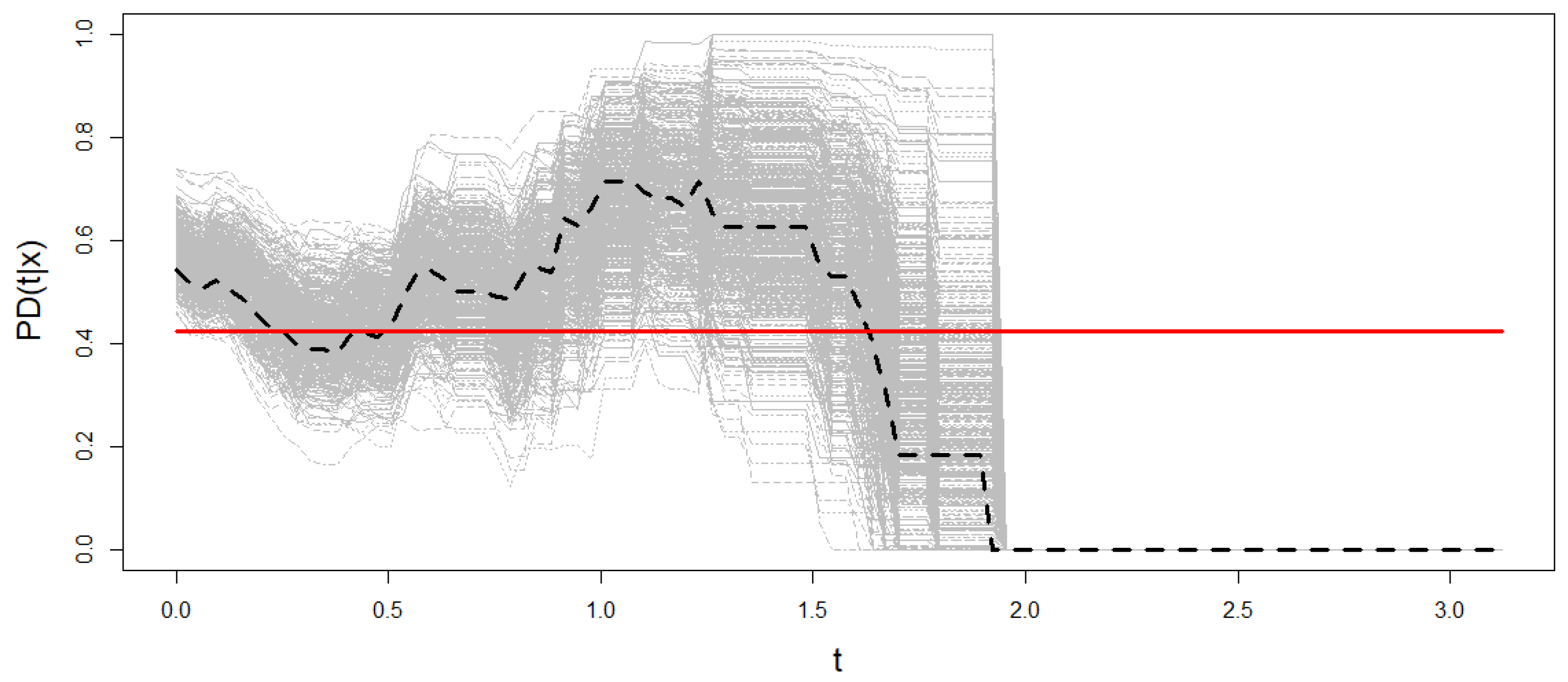
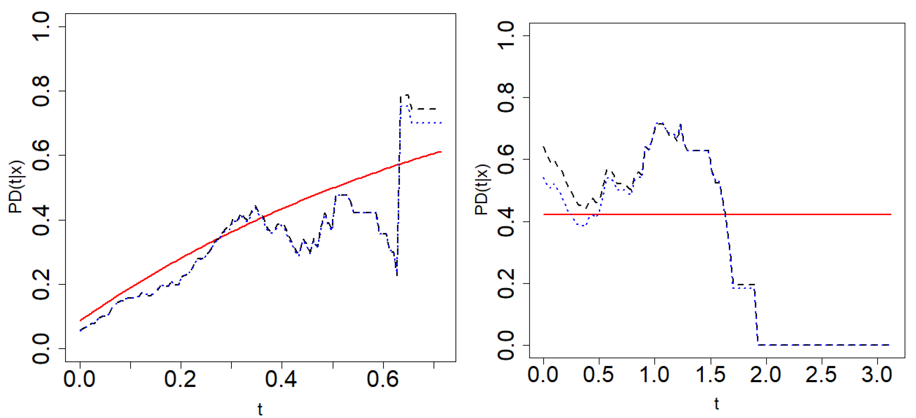
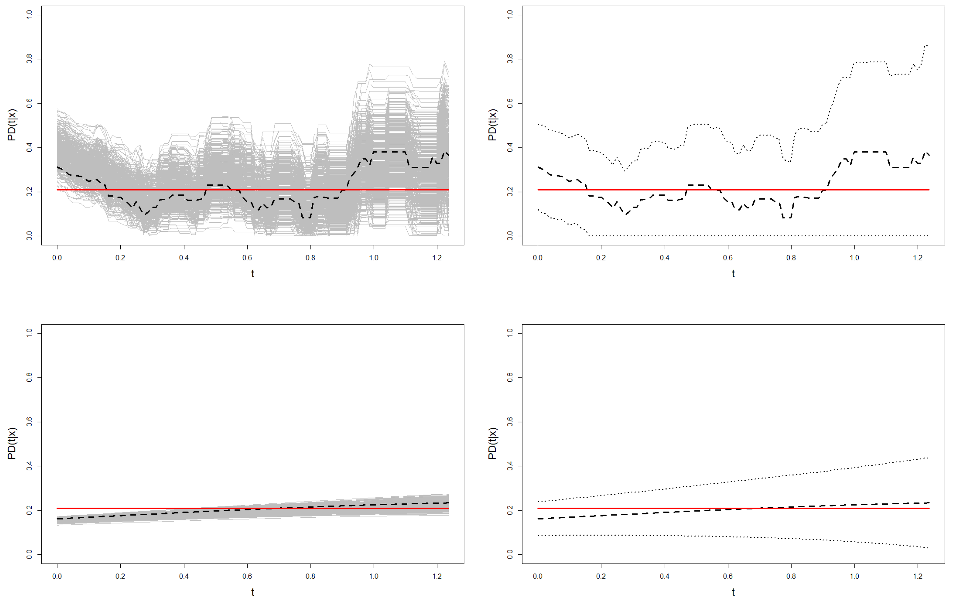
Figure 8 shows Beran’s estimations of the PD for
resamples from one sample of Model 2 when the conditional probability of censoring is 0.5. The theoretical probability of default is also plotted in the figure. The PD is estimated on a time grid
such that
. The information provided by the data in the right tail of such a time distribution is sparse due to high censoring. The method results in extremely wide confidence regions or degeneration to zero as in the case of Model 2 (see
Figure 8). Therefore, the time grid in this section is restricted to the interval where sufficient information is available.
For this section, we consider the problem of obtaining the bootstrap confidence region for the probability of default in a time grid
such that with
for all
and
, with
b being approximately equal to
of the grid length. For Model 1, having set the value of the covariate,
, the time horizon is
(
of the time range) and
. For Model 2, having set the value of the covariate,
, the time horizon is
(
of the time range) and
.
Table 4 contains the bandwidths that minimize the
MISE function for Beran’s estimator and the smoothed Beran’s estimator along this new time grid.
For each model, the confidence region is obtained according to the method explained in
Section 4 using both Beran’s estimator and the smoothed Beran’s estimator. The criteria for comparing the methods are set out below.
A confidence region performs well if its coverage is close to the nominal one, in this case , and has a small area or average width. Denoting and when using Beran’s estimator or and when using the smoothed Beran’s estimator, the following values measure the performance of the confidence region and allow for the comparison of results.
Coverage is the percentage of bootstrap regions that contain the whole theoretical probability of default curve and it is defined as follows
The mean pointwise coverage is the mean of the proportion of time grid values for which the confidence region contains the theoretical probability of default curve. It is given by
Average width of the bootstrap confidence region is defined by
Winkler score (see [
30]) is also used to compare the behavior of the methods. For classical confidence or prediction intervals, it is defined as the length of the interval plus a penalty if the theoretical value is outside the interval. Thus, it combines width and coverage. For values that fall within the interval, the Winkler score is simply the length of the interval. So low scores are associated with narrow intervals. When the theoretical value falls outside the interval, the penalty is proportional to how far the observation is from the interval. The formula of the Winkler score (WS) as a function of the time and covariate variables is as follows:
Since we are working with confidence regions for fixed
and
t varying over the interval
, the integrated Winkle score is proposed as a criteria for the comparison of the confidence regions. It is defined by
and the lower the value of IWS, the better the performance of the confidence region.
The results obtained are shown in
Table 5. The high values of pointwise coverage in all scenarios are remarkable. Furthermore, these coverage percentages are preserved when using double smoothing, while the average width of the confidence regions is halved. This is reflected in the IWS, which presents much larger values in the Beran’s estimator-based confidence regions.
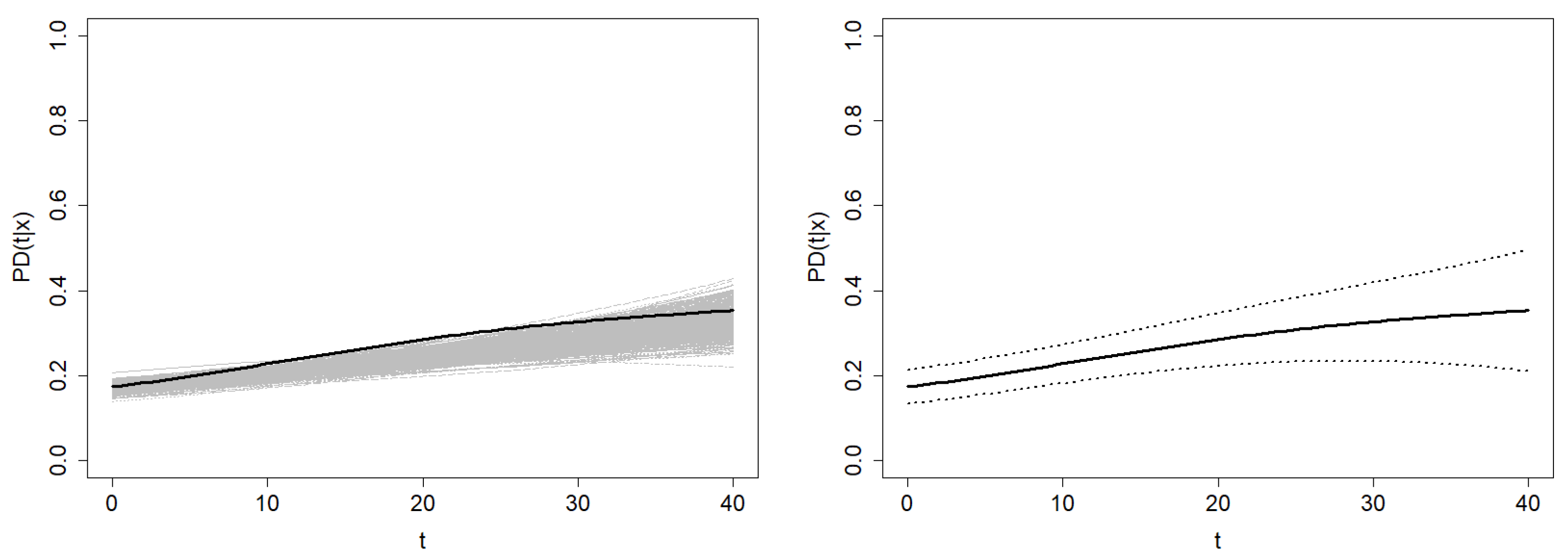
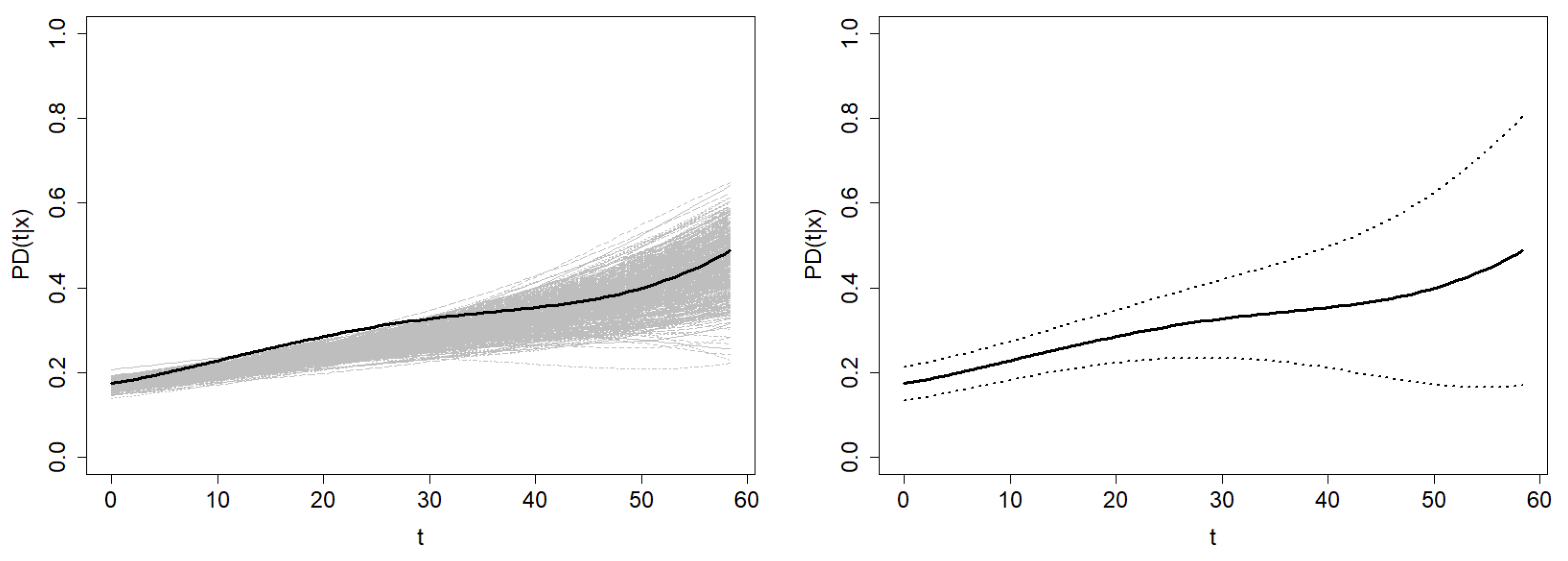
This analysis is also illustrated in
Figure 9 and
Figure 10, where the confidence region for the probability of default of one sample from Models 1 and 2 is shown. These graphs show the higher variability of the Beran’s estimations in the resamples with respect to the smoothed Beran’s estimations. This leads to much wider confidence regions, especially at the right tail of the time distribution.
6. Application to Real Data
In this section, bandwidth selectors for Beran’s and the smoothed Beran’s estimators are applied to the German Credit dataset, and the confidence region of the probability of default is obtained. This dataset is publicly available on the webpage
http://archive.ics.uci.edu/ml/datasets/Statlog+(German+Credit+Data) (accessed on 15 September 2021) and was previously analyzed in [
31]. It includes information about 1000 credits, from which 293 were classified as bad credits and 707 as good credits. Then, the censoring ratio of this dataset is
. The duration of the credits in months is available along with the credit amount, checking account, savings amount and time of employment, among others.
The duration of the credits is set as the time to default, Z, the bad/defaulted credits are denoted by and the good credits by . Let us denote the credit scoring with .
Since some of the original covariates are ordinal (interval) variables, we change them into numerical variables by following the criteria explained in [
31]:
is already a continuous variable denoting amount of credit in DM,
denotes the amount of money in the checking account in thousands of DM,
denotes the savings amount in thousands of DM, and
denotes the years of employment. The single-index method proposed by [
31] is used to estimate
. The credit scoring is obtained as follows:
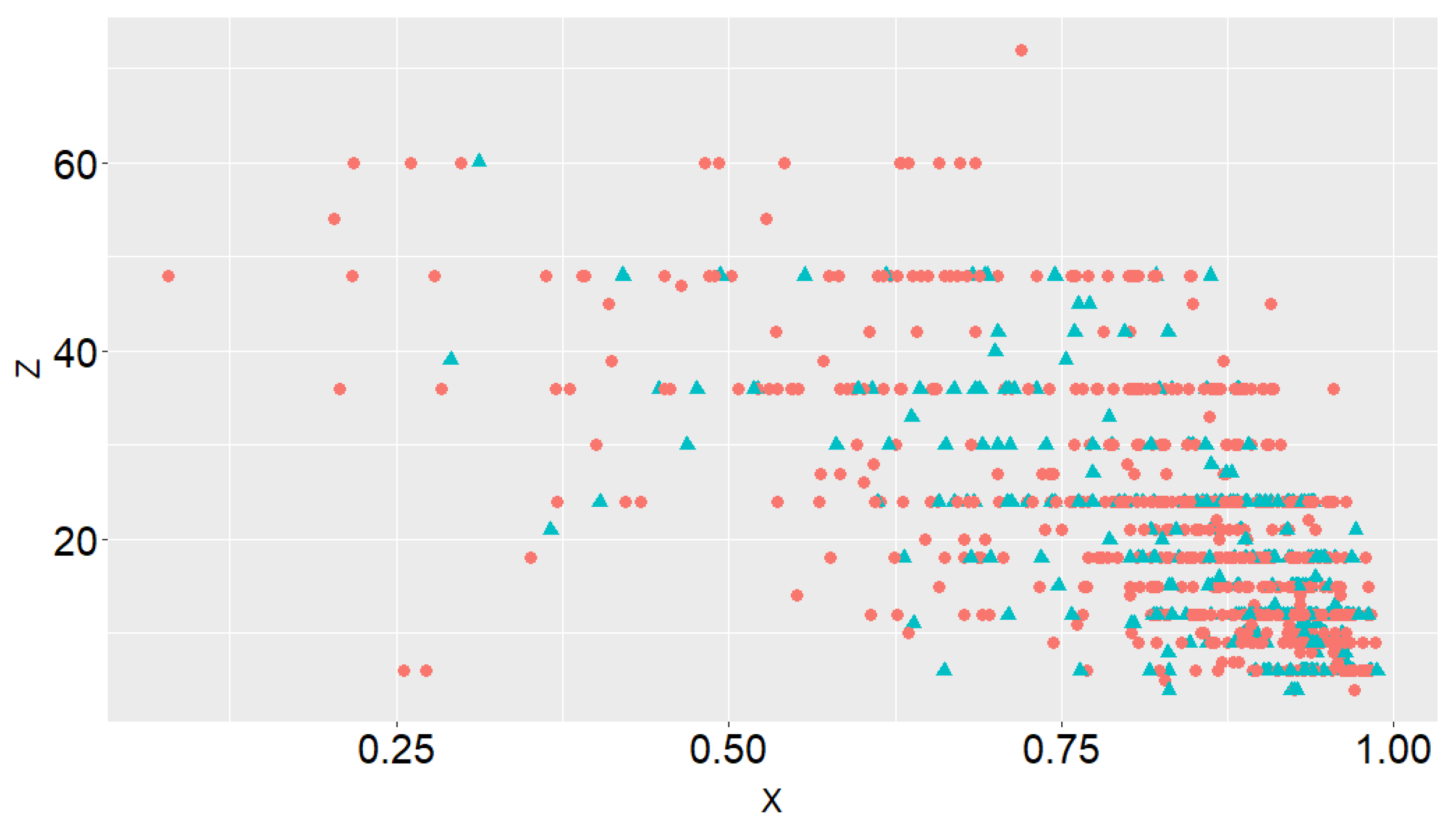
Figure 11 shows the scatter plot between credit scoring and follow-up time variable by distinguishing between the censored and uncensored (and therefore, defaulted) credits. A dependency relationship between the two variables can be identified in the plot.
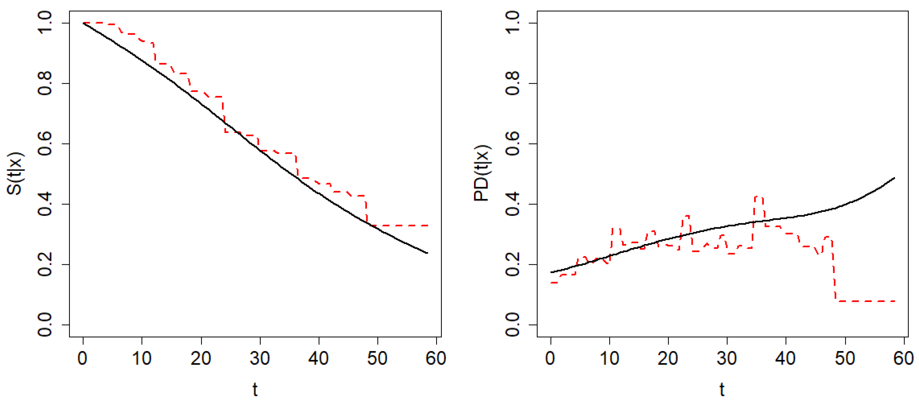
The probability of default,
, is estimated when
, which is a close value to the sample mean of the credit scoring, and
. The bandwidth selector presented in
Section 2.1 is used to approximate the optimal bandwidth for Beran’s estimator, obtaining
. The bandwidth selector presented in
Section 2.2 gives the bootstrap approximation of the optimal bivariate bandwidth for the smoothed Beran’s estimator,
. The estimations of the conditional survival function and the probability of default by means of Beran’s and the smoothed Beran’s estimator with the corresponding bootstrap bandwidths are shown in
Figure 12. The poor behavior of Beran’s PD estimator for large values of time is evident. The results obtained by the doubly smoothed Beran’s estimator seem to be more appropriate, since the roughness of the Beran’s estimaton is not expected in this type of curve. Supporting the conclusion of our real data analysis, the estimation of the probability of default over time for the assessment of risk in portfolios and bond rating obtained in [
32,
33] have shapes similar to those obtained here.
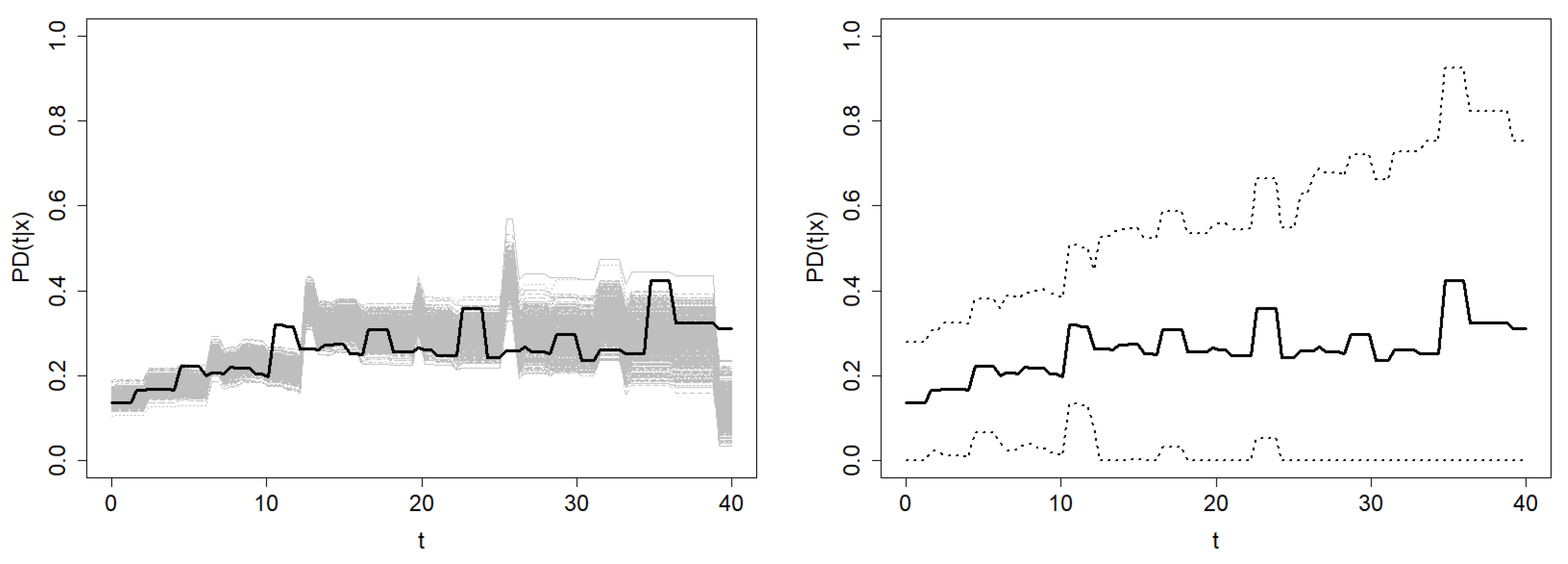
Finally, the confidence region methods proposed in
Section 4 are applied. Since the
MISE bandwidths are unknown in this context, bootstrap bandwidths are used. The bootstrap resamples and the resulting confidence regions at confidence level
using each estimator are shown in
Figure 13. The average width of the confidence region based on Beran’s estimator is
, and the average width of the one based on the smoothed Beran’s estimator is
. Note that the confidence region of
is computed over the time interval
. Since the information provided in the right tail of the time distribution is sparse, Beran’s estimator performs very poorly, leading to extremely wide confidence regions. However, this problem is not as severe for the doubly smoothed Beran’s estimator, so the confidence region is computable for higher values of time.
Figure 14 shows the confidence region of
based on the smoothed Beran’s estimator with
. The average width of this confidence region is
.
In practice, the financial institution measures different features of its clients, such as age, amount of money in the bank account, salary, years of employment, etc. They summarize, usually by logistic regression, these covariates into the single variable credit scoring. Subsequently, techniques such as those shown in this paper allow the calculation of the probability of default at horizon b for all of them. The curve provides the probability that the client will default after a certain period of time b.
7. Conclusions and Future Lines
This article proposes an automatic bandwidth selector and confidence regions algorithms based on bootstrap selectors for Beran’s estimator and the smoothed Beran’s estimator of the probability of default in credit risk. The proposed resampling methods and bootstrap selectors allow to approximate the MISE bandwidths corresponding to each estimator: the covariate-smoothing bandwidth in the case of the Beran estimator and the two-dimensional covariate and time-smoothing bandwidth in the case of the doubly-smoothed estimator. In view of the simulation study carried out, it can be concluded that the bandwidth selectors work properly. The doubly smoothed Beran’s estimator with bootstrap bandwidths commits smaller estimation errors than Beran’s estimator. The simulation results also show the good behavior of the confidence regions, especially those based on the doubly smoothed Beran’s estimator. They have a lower average width, reducing the uncertainty about where the true probability of default curve is located, while preserving a high coverage.
The main limitation of proposed methods is their high computational cost. Approximating the bootstrap bandwidth or computing a confidence region by 500 resamples from a sample of size 100 requires one minute, while a sample of size 500 requires 25 min to obtain the result. These times are similar for both estimators. They seem to increase quadratically as the sample size grows, which may lead to prohibitive times for very large sample sizes. Using subsampling techniques is an appealing idea to be considered in the future for optimizing these methods.
In a financial context, credit scoring typically summarizes several interesting features of clients in order to measure their creditworthiness. However, this work could be extended to the case of having a multidimensional covariate
, where each
is a feature of the individual. Methods such as single-index can be useful for this purpose to avoid the curse of dimensionality. An approach along the lines similar to [
31] can be used.


