The Impact of COVID-19 on the Connectedness of Stock Index in ASEAN+3 Economies

Abstract

This paper explores the impact of the COVID-19 pandemic on the connectedness of stock indexes in the group of developed and emerging economies known as the ASEAN+3. We derived our empirical findings from the Diebold and Yilmaz (DY12) and Baruník and Křehlík (BK18) spillover methods, using daily data from 10 May 2005 to 24 February 2021. We show that the COVID-19 pandemic has had a bigger impact on the return and volatilities of ASEAN+3 stock markets than previous economic turmoil, such as the 2008 global financial crisis and the 2009–2012 European debt crisis. Using a frequency domain methodology, we find evidence that return spillovers mostly occur in the short-term, while volatility connectedness is more pronounced in the long-term. The Singapore stock market primarily acts the as top transmitter in returns and volatilities, whereas Vietnam has become the top receiver of shocks in returns. We also demonstrate that it is possible to replicate the frequency-domain connectedness measures of BK18 with a DY12 methodology. Using a series decomposed with a wavelet-based approach, we find that the total spillover indices for short-, medium-, and long-term frequencies computed with the DY12 approach are comparable to the within connectedness indices of BK18. Our results have important policy implications for investors, regulators, and policy makers.

1. Introduction

An economic crisis can have a direct or indirect impact on a country’s economy. If one country’s stock market is highly correlated with another, the financial stability of the former is influenced by the financial stability of the latter. As a result, a strong or close relationship between markets increases the vulnerability to external shocks and can affect the economic conditions of the respective countries. A recent study by [1] revealed that potentialities to diversify investment and take on risks across international markets are a critical consequence of the interconnectedness between markets. As a result, analyzing the interconnectedness of financial assets, particularly stocks, is important for investors, since it enables them to analyze the effects and decide effectively on opportunities regarding international portfolio diversification.

Previous studies that examined the relationships of financial markets have shown that financial strain and crises are directly impacted by the gravity and extent of connectedness between those markets; with examples being drawn from previous crises such as the global financial crisis (GFC), the debt crisis in Europe [2,3], and the COVID-19 health crises [4,5,6,7,8,9,10]. Recent articles on the financial impact of COVID-19 have reported varying results for different stock markets. For example, it was shown that COVID-19 has been far more destructive to the US stock market than previous infectious diseases [11]; and the entities listed in the US stock market have exhibited a higher reactivity to the recent COVID crisis compared to their Asian and Australian counterparts [12]. However, ref. [6] revealed that Asian stock markets have been more affected than European ones. Similarly, ref. [13] explored the pre- and during COVID-19 spillovers between crude oil prices and five developed stock markets in Europe, concluding that spillovers were more apparent during the COVID-19 period. In addition to a significant decline in stock indices [14], the pandemic also created a dynamic whereby the stock exchanges were highly uncertain and extremely susceptible to movements [15,16], leading to huge investment losses [17].

A variety of models have been used in the empirical literature to examine connectedness, including cross-market correlation coefficients [18,19], multivariate ARCH and GARCH models [20,21], cointegration techniques [22], vector autoregressive (VAR) model [23,24], and wavelet methods [7,25]. However, one of the most notable empirical methods is that of Diebold and Yilmaz [26,27,28], who proposed a set of connectedness measures based on the concept of forecast error variance decomposition derived from rolling-window VARs. Their method has already attracted considerable attention from academic researchers and has been applied to a wide range of issues, including stock market interdependencies. For example, Diebold and Yilmaz’s [27] methodology (henceforth DY12) was applied in [29] to calculate the balance of equity and volatility returns between MENA (Middle East and North Africa) and US stock markets, prior and after the global financial crisis. They mentioned that the relationship with the US stock market was very weak prior to the crisis period, but that it was bound to a high degree after the crisis. The DY12 approach was utilized in [30] to examine the relationship between global stock markets and GIPSI (Greece, Ireland, Portugal, Spain, and Italy). The connection between these two was examined using two methods—static and rolling-window methods—and it was found that there was an element of intra-financial reactivity between the global stock markets and GIPSI when COVID-19 hit. Pursuant to this, [31] applied a DY12 spillover index methodology to examine the intersectionality of spillovers between the global stock markets and ASEAN-5. The authors also found that the relationship of spillovers was positive.

The DY12 methodology provides a clear and intuitive aggregate of interdependence, in terms of asset returns and magnitude of volatilities, by applying the broad-based VAR framework of Koop et al. [32] and Pesaran and Shin [33], and generating a variance decomposition that is not influenced by the ordering. To this end, Baruník and Křehlík [34] (henceforth BK18) extended the spillover index of DY12 from the time series domain to the frequency domain. The BK18 framework allows a deeper and more comprehensive insight into the connectedness across different time horizons, as it offers a coherent structure for quantifying the magnitude and direction of connectedness, through a set of variables over the time at which different spillovers occur. This method has gained great interest from recent researchers, see for example [31,35,36,37], to study the connectedness of different financial assets.

Therefore, the purpose of this study was to analyze the impact of COVID-19 on stock index returns and volatilities among ASEAN+3 (APT) economies. The APT block comprises ten ASEAN member states and three East Asian countries (China, Japan, and South Korea). ASEAN is considered to be the strongest and most successful regional grouping in the developing world, and its strong economic performance has made ASEAN one of the most active regions in the world [38]. Among ASEAN countries, we include the top five ASEAN countries, namely Indonesia, Malaysia, the Philippines, Singapore, and Thailand (ASEAN-5), as well as Vietnam. The inclusion of Vietnam is deemed inevitable and necessary. Indeed, ref. [39] argued that Vietnam has had a successful track record of avoiding recessions in recent years, and in doing so, has helped to prevent the ripple effects of recession from the shores of other Asian countries. In fact, the International Monetary Fund (IMF)’s identification of Vietnam as one of Asia’s fastest-growing economies in 2020 was also considered when including it in the analysis. Thus, this block is a unique sample with which to analyze the impact of COVID-19 shocks on stock index connectedness among developed and developing countries.

Our study contributes to the existing literature in three ways. First, our sample includes the most recent crises of the COVID-19 pandemic, which has had a huge impact on the world economy, especially stock markets. The analysis of measuring returns and volatility spillover between stock markets has become very important, for monitoring the extent of the COVID-19 impacts on equity markets and to issue early warnings to investors.

Second, we use the approaches of both DY12 and BK18 to find the dynamic connectedness of stock indexes in six ASEAN countries, including China, Japan, and South Korea. To the best of our knowledge, our study is the first paper to analyze the impact of the COVID-19 outbreak across these countries, and encompassing both time and frequency domains. Unlike the conventional time series methods, such as Johansen cointegration or Granger causality, which obtain static measurements for one or more variables captured over a period in a given space (a specific country, state, and so on), the DY12 and BK18 procedures allow us to identify and quantify the direction and degree of spillovers between markets over time and across investment horizons simultaneously. As such, these procedures are considered superior to the classical time series approach because they enable the identification and quantification of returns and volatility interconnectedness across markets. In the same vein, our study complements and extends the previous work of [40], who employed the time-domain connectedness to measure the ASEAN+3 stock market spillover from 1999 to 2019. The frequency-domain approach of BK18 is expected to provide more detailed results. This is important in helping investors decide on the duration of their investments.

Third, we measure stock market connectedness in terms of returns and volatility. Previous studies, such as [37,41], only examined connectedness separately, either in returns or in volatility. Since there is growing evidence (see [36,42], as examples) that return and volatility spillovers for stock markets differ (moving in opposite direction) over the short-, medium-, and long-term, it is critical for us to provide further evidence of this. Additional information will help investors to mitigate risks and policymakers to establish regulations, to reduce the impact of the pandemic on the economy.

Fourth, we use a wavelet approach to decompose our data, according to three distinct frequencies: short-, medium-, and long-term, and employ the DY12 method to estimate the connectedness index. This approach aims to replicate the within connectedness index of BK18 and to determine if we can use DY12 method to estimate frequency-based spillover index as a robustness check for the BK18 method. In previous research exploring the relationship between dynamic connectedness across a spectrum of stock markets, this type of analysis has not been employed.

Our result shows that in the time domain, the total connectedness of stock index returns is higher than total connectedness in the volatility of stock indexes. In terms of the frequency domain, our result shows that the return shocks emanating from one market, then being imparted to other markets, only produce short-term effects. In contrast, the volatility shocks arising from one market and transferred to other markets trigger long-circulating effects. Our results also suggest that Singapore primarily acts as spillover transmitter for both returns and volatilities. Meanwhile, Vietnam has become the top receiver of spillover, in terms of returns, while the Philippines is the top receiver based on the volatility of stock indexes. Furthermore, our results also reveal that the long-term frequency connectedness was particularly intense in 2020, where the spillover surged considerably owing to COVID-19. This indicates a strong impact and long-lasting spillover effects of COVID-19 among ASEAN+3 economies. Last, the robustness test revealed that the use of decomposed data with the wavelet approach in the DY12 method can replicate the within connectedness index of BK18. The total spillover indices for short-, medium-, and long-term frequencies are comparable for both methodologies.

The rest of the paper is organized as follows: The relevant literature is presented in Section 2. Section 3 describes the DY12 and BK18 methods, followed by an overview of the data and our methodology. Section 4 presents the empirical results. Section 5 provides some concluding thoughts.

2. Literature Review

The very first COVID-19 case was reported in Wuhan, China, on 31 December 2019. As a result of being highly infectious, the World Health Organization (WHO) issued an alert on 30 January 2020; and later on 11 March 2020, it was declared a pandemic. Over time, its concentration has shifted from China to other regions in Asia, Europe, and the Americas. The immediate solution to preventing its spread was isolation, and a lockdown was applied in most countries. According to The Economist [43], this pandemic is a serious threat to global markets. In addition, news about COVID-19 in international media caused negative feelings, fear, and uncertainty [44]. As a result, this uncertainty could affect stock market returns.

Changes in stock market returns and volatility and subsequent contagion through the transfer of information across local and international markets during the crisis have received considerable attention from academics, policy makers, and investors [45]. The ability and accessibility of information enabling investors to discern and comprehend the magnitudes of return, as well as the volatility triggered by pandemic jolts and situational crises, is critical in order for them to deflect all potential risks when considering an investment. This is particularly true when pandemics such as the COVID-19 strike a pervasive blow, and legislators need to devise measures and other guidelines which can minimize the economic repercussions after such a pandemic. Using a GARCH (1,1) model, ref. [46] examined the impact of the COVID-19 pandemic and related deaths on the US stock market (Dow Jones and S&P500 indices). The authors ascertained that the death toll reports in Italy and France precipitated adverse effects on US stock market returns, but prompted a promising impact on returns of VIX. In addition, ref. [47] measured the shock impacts resulting from COVID-19 on the stock exchange in China, by applying an analysis of available panel data. The conclusion derived was that, between 10 January to 16 March 2020, the reported increase of total deaths caused by COVID-19 daily, as well as confirmed COVID-19 related cases, sparked off a series of adverse impacts pertaining to the returns of stock in every company listed in the Hang Seng and Shanghai Stock Exchange Composite indexes, respectively. Furthermore, ref. [48] also examined the immediate and direct consequences of COVID-19 vis-à-vis the volatility in the European, Asian, United States, and Australian stock exchanges, as well as the more hidden and indirect impacts, by relying on the panel data obtained. Their findings suggested that Google-based fear of COVID-19’s contagious effects would result in heightened aversion to risk in the stock market. Using the DOW Jones World Index and Islamic Sukuk Index data, ref. [8] argued that Islamic bonds had the potential to be a safe haven during the ongoing COVID-19 crisis. The authors also argued that spillovers between conventional and Islamic stock markets increased during this period. A recent study by [42] explored the interrelatedness of the crude oil market, and the stock markets in US, Japan, and Germany, in its intersectionality with the COVID-19 crisis. They asserted that the aftereffects of COVID-19 have led to an unprecedented degree of risk, simultaneously triggering the circuit breaker within the US stock market in four separate incidents. The aftermath of this unprecedented event brought about severe and unparalleled losses to investors within a short time span. Moreover, COVID-19 has had greater ramifications for oil and stock market volatility compared to the backwash brought about by the global financial crisis in 2008. Investigating cross-correlations for 80 cryptocurrencies over the course of the COVID-19 outbreak, ref. [49] concluded that cryptocurrencies are now more highly cross-correlated with one another than they were previously. Their findings also demonstrated that during pandemic periods, the cryptocurrency market exhibits higher degrees of cross-correlations with the stock, commodity, and foreign exchange markets.

Previous studies have focused more on the spillover effects during the COVID-19 pandemic on the developed stock market, with less attention on emerging countries, such as ASEAN, with the world stock index. A recent study on the impact of COVID-19 on ASEAN countries, ref. [9] revealed that the pre- and actual lockdown spillovers effects observed in Vietnam’s stock performance are diametrically opposed. While stock performance was significant and positive during the actual lockdown across the whole business spectrum, the opposite was true prior to the lockdown. Prior to the lockdown, the stock returns were significant and negative. More recently, ref. [10] used a wavelet approach to reveal the impact of COVID-19 on ASEAN-5 countries and the Dow Jones Index. Their results demonstrate a three-period progression in the connection between ASEAN-5 countries and the Down Jones: at the start of the COVID-19 outbreak, Malaysia, Indonesia, and Singapore’s equities exhibited strong reactivity to the Dow Jones; mid-outbreak, Thailand and the Philippines exhibited consistency with the Dow Jones; and finally, as the COVID-19 crisis panned out across the year, all equities in the ASEAN-5 exhibited a consistent and parallel coherence with the Dow Jones Index.

Against the backdrop of worldwide economic turmoil, the momentum of trade between ASEAN and the plus three countries (China, Japan, Korea) has remained steady. This is evident from the increase of ASEAN total merchandise trade with the plus three countries; recorded at 31 percent, equivalent to USD 37.9 billion. This translates to a total of USD 37.9 billion of foreign direct investment (FDI) flows from the plus three into ASEAN, up 9.9 percent from the previous year [50]. This gives some motivation to study the connectedness of stock market among APT countries, which can help investors to make sound investment decisions. There have been some studies that investigated the integration of the plus three country stock markets with ASEAN stock markets. For example, ref. [40] explored the level of market interconnectedness between ASEAN-5 and the plus three countries, using the VAR method and rolling window approach. He concluded that the markets’ inter-reactivity and integration are high. Furthermore, ref. [51] found that during the Chinese stock market crash in 2015, the financial market integration between ASEAN-5 and Chinese markets rose to 533%. Other research also supported the argument that Asian markets tend to integrate in turbulent periods; see [52,53]. As stated in the introduction, we are aware of no studies that have discussed the connectedness of stock market index returns and volatility among APT economies, particularly during COVID-19 pandemic, and in the hope of providing useful implications for both policymakers and market participants.

3. Method

We constructed a spillover index for ASEAN+3 financial markets, with nine countries in total, by adopting the methodology of DY12 and BK18. The focus was to compute the forecast error variance decomposition (FEVD), to examine the spillover index.

3.1. Diebold and Yilmaz (DY12) Time Domain Approach

To examine the cross-market interdependencies spillovers in the time domain, the generalized vector autoregression (GVAR) framework developed by DY12 was applied in our analysis. This framework hinges on the generalized forecast error variance decompositions (GFEVD), to compute the indexes of total, directional, and net spillovers. Following [27,28], the definition of the K-variable, VAR (p) system, is:

$$y_t=c+A_1{y}_{t-1}+A_2{y}_{t-2}+\dots +A_p{y}_{t-p}+u_t$$

(1)

where $y_t$ stands for the $K\times 1$ vector of variables at time $t,$ and $c$ represents the constants of the $K\times 1$ vector of variables. The coefficients of the $K\times K$ dimension matrix are denoted by $A$. A simpler form of Equation (1) above is:

$$Y_t=C+A{Y}_{t-1}+U_t$$

(2)

where $A$ signifies a $pK\times pK$ dimensional matrix; and $Y,C$, and $U$ signify $pK\times$ 1 vectors, as defined below:

$$Y=\left[\begin{array}{l}{y}_t\hfill \\ y_{t-1}\hfill \\ ⋮\hfill \\ y_{t-p}\hfill \end{array}\right],C=\left[\begin{array}{l}c\hfill \\ 0\hfill \\ ⋮\hfill \\ 0\hfill \end{array}\right],A=\left[\begin{array}{ccccc}{A}_1& A_2& \cdots & & A_{p-1}{A}_p\\ I_K& 0& \cdots & 0& 0\\ 0& I_K& 0& 0& ⋮\\ ⋮& \ddots & ⋮& ⋮& ⋮\\ 0& 0& \cdots & I_K& 0\end{array}\right],U=\left[\begin{array}{l}{u}_t\hfill \\ 0\hfill \\ ⋮\hfill \\ 0\hfill \end{array}\right]$$

(3)

We employ variance decomposition in the VAR model estimation to evaluate the extent to which one variable influences or contributes to other variables, for explaining the variation across variables. The H-step forecast of the mean square error (MSE) of variable $y_t$ is given by:

$$\mathrm{MSE}|y_{i.t}(H)|={\displaystyle \sum {}_{j=0}^{H-1}}{\displaystyle \sum {}_{k=1}^k}{(e_i^{\prime }{\Theta }_j{e}_k)}^2$$

(4)

where $e_i$ represents the $i$-th column of $I_K,{\mathsf{\Theta }}_j={\mathsf{\Phi }}_{j}P,$ and $P$ denotes the lower triangular matrix. To estimate $P$, the lower triangular matrix, we use the generalised decomposition of the variance covariance matrix ${\mathsf{\Omega }}_u=E\left(u_t{u}_t^{\prime }\right)$ following [32,33]. In addition, $\mathsf{\Phi }=J{A}^j{J}^{\prime },$ where $J=\left|I_K,0,\dots ,0\right|$. We estimate $k$’s contribution to variable $i$ as:

$${\theta }_{ik,H}={\displaystyle \sum {}_{j=0}^{H-1}}{(e_i^{\prime }{\Theta }_j{e}_k)}^2/MSE\lfloor y_{i,t}(H)|$$

(5)

We estimate the dependency of the variables in the system to abridge all items in (H) from 1 to $K$ using [27]. We define connectedness as follows:

$$C_H=\frac{1}{K}{\displaystyle \sum {}_{ij=1}^K}{\theta }_{ij}^H(i\ne j)$$

(6)

To ensure that the estimated total connectedness among the variables spans between 0 and 1, Equation (6) excludes any diagonal elements from the system. This measurement, thus, investigates the extent to which the contribution of the system’s components to variations is initiated by another variable, rather than the variable itself. A value of 0 implies that the system’s components are independent, with no spillover effects. When the value is one, this indicates that the system’s components are strongly connected.

3.2. Baruník and Křehlík (BK18) Frequency Domain Approach

Extending the GFEVD framework, BK18 builds upon the DY12 time domain methodology to examine connectedness at various frequencies, namely the short-, medium-, and long-term. We examine the frequency response obtained as a Fourier transformation of the coefficient $\Psi (e^{-i\omega })={\displaystyle {\sum }_h{e}^{-i\omega h}}{\Psi }_h$, with $i=\sqrt{-1}$. By using the frequency response functions from the spectral representation, the generalized variance decomposition at the given $\omega \in \left(-\pi ,\pi \right)$ is defined as:

$${(f\left(\omega \right))}_{j,k}\equiv \frac{{\sigma }_{kk}^{-1}\mid ({{\left(\mathsf{\Psi }\left(e^{-i\omega }\right)\sum \right)}_{j,k}\left)\right|}^2}{\left(\mathsf{\Psi }\left(e^{-i\omega }\right)\sum {\mathsf{\Psi }}^{\prime }{\left(e^{+i\omega }\right)}_{j,j}\right)}$$

(7)

where $\Psi (e^{-i\omega })={\displaystyle {\sum }_h{e}^{-i\omega h}}{\Psi }_h$, indicates the Fourier transformation of the impulse response function $\mathsf{\Psi }$ and ${(f\left(\omega \right))}_{j,k},$ which signifies the part of the spectrum of the $j$-th variable under the frequency $\omega$, as a result of shock in the k-th variable. Assuming that the denominator holds the spectrum of the $j$-th variable under frequency $\omega$, we deduce Equation (7) above as the quantity within the frequency causation. The generalized decomposition of the variance is obtained under the frequency omega, by weighting the function ${(f\left(\omega \right))}_{j,k}$ by the $j$-th variable frequency share of the variance. Following the above, the weighting function is:

$${\Gamma }_j=\frac{{(\Psi (e^{-i\omega }){\displaystyle \sum {\Psi }^{\prime }(e^{+i\omega })})}_{j,j}}{\frac{1}{2\pi }{\displaystyle {\int }_{-\pi }^{\pi }{(\Psi (e^{-i\lambda }){\displaystyle \sum {\Psi }^{\prime }(e^{+i\lambda })})}_{j,j}d\lambda }}$$

(8)

Equation (9) shows j-th variable power in the system under frequency $\omega$ and sums the frequencies to a constant value of $2\pi .$ It is noteworthy that even though the Fourier transformation of the impulse response is a complex number, the generalized spectrum is the squared coefficient of the weighted complex number and, as result, is a real number. We set the weighted complex number and, as result, this is a real number. We set the frequency band formally as: $d=\left(a,b\right):a,b\in \left(-\pi ,\pi \right),a<b$. In Equation (9), the generalized variance decomposition under the frequency band d is:

$${({\Theta }_d)}_{j,k}=\frac{1}{2\pi }{\displaystyle {\int }_d^{\infty }{\Gamma }_j}(\omega ){(f(\omega ))}_{j,k}d\omega .$$

(9)

The generalized variance decomposition is scaled under the frequency band $d=\left(a,b\right):a,b\in \left(-\pi ,\pi \right),a<b$, as shown in Equation (10):

$${({\tilde{\Theta }}_d)}_{j,k}=\frac{{({\Theta }_d)}_{j,k}}{{\displaystyle {\sum }_k}}{\left({\Theta }_{\infty }\right)}_{j,k}$$

(10)

Under the frequency band $d,$ we evaluate the intra-market dependency on the connectedness by formulating the unweighted within connectedness, as follows:

$$C_d^W=100\cdot \left(1-\frac{\mathrm{Tr}\left\{{\tilde{\mathsf{\Theta }}}_d\right\}}{\sum {\tilde{\mathsf{\Theta }}}_d}\right)$$

(11)

Within connectedness calculates the connectedness that occurs within the frequency range, without considering the impact of variation in this band in relation to other variations. Connectedness within frequency bands can be described as pure unweighted connectedness, where information beyond the perceived band is disregarded. The primary reason for our consideration of the within connectedness is to investigate the impact of cross-sectional dependence of samples. To obtain the frequency connectedness at band $d$, $C_d^F$ is specified as:

$$C_d^F=100\cdot \left(\frac{\sum {\tilde{\mathsf{\Theta }}}_d}{\sum {\tilde{\mathsf{\Theta }}}_{\infty }}-\frac{\mathrm{Tr}\left\{{\tilde{\mathsf{\Theta }}}_d\right\}}{\sum {\tilde{\mathsf{\Theta }}}_{\infty }}\right)=C_d^W\frac{\sum {\tilde{\mathsf{\Theta }}}_d}{\sum {\tilde{\mathsf{\Theta }}}_{\infty }}$$

(12)

To sum up, frequency connectedness permits the original DY12 connectedness index to be decomposed into various parts. As a result, when applying the BK18 method, the total spillover index proposed by DY12 is obtained by summing the connectedness across all frequency bands. In addition, by calculating measures for directional connectedness, the total connectedness across all bands of frequency is applied. This includes directional frequency connectedness from the other variables to the i-th variable or from the i-th variable to the rest of the variables.

3.3. Wavelet-Based Method

We estimate the wavelets for returns and volatility in the time domain using the maximal overlap discrete wavelet transform (MODWT). The MODWT wavelet and scaling coefficient ${\tilde{w}}_{j,t}$ is defined as:

$${\tilde{w}}_{j,t}=\frac{1}{2^{j/2}}{\displaystyle \sum {}_{l=0}^{L-1}}{\tilde{h}}_{j,l}{r}_{t-j}$$

(13)

and ${\tilde{v}}_{j,t}$ for a return and volatility series $r\left(t\right)$ is written as:

$${\tilde{v}}_{j,t}=\frac{1}{2^{j/2}}{\displaystyle \sum {}_{l=0}^{L-1}}{\tilde{g}}_{j,t}{r}_{t-j}$$

(14)

where $L$ is the length of the filter. With the application of the least asymmetric wavelet technique [54,55], the return and volatility series’ multiscale decomposition with a filter length of $L=8$ is derived. The decomposed signals of the multiresolution analysis in the MODWT are further derived herein, as follows:

$$r(t)=W_J(t)+{\displaystyle \sum {}_{j=1}^J}{D}_j(t)$$

(15)

where $W_J(t)={\displaystyle \sum {}_{l=-\infty }^{+\infty }}h(l)W_{(J-1)}(t+2^{j-1}\times l)$ denotes the smoothed version of the series $r\left(t\right)$ at scale $J,$ and $D_j(t)={\displaystyle \sum {}_{l=-\infty }^{+\infty }}g(l)W_{j-1}(t+2^{j-1}\times l)$ presents the wavelet scales, which indicates the local fluctuation over the period of returns as each scale $j$. Furthermore, the return and volatilities series are decomposed into six wavelet scales $W\left(D_1,\dots ,D_6\right)$. Following [37], we convert the decomposed series into three frequency domains, where the short-term horizon is defined as the sum of the $D_1$ and $D_2$ series, the medium-term horizon is defined as the sum of $D_3$ and $D_4$, and the long-term horizon is the sum of $D_5$ and $D_6$.

3.4. Data and Variables

To investigate the interconnectedness of ASEAN+3 financial markets, we employed daily data from 10 May 2005 to 24 February 2021, which spans many volatile phases and disturbances, including sharp swings in commodity futures markets and significant global incidents, such as the 2008–2009 GFC, the oil price crisis that started in 2014, and the ongoing COVID-19 global pandemic. The stock market indices of the ASEAN+3 countries include Singapore (SG), Indonesia (IDN), Japan (JPN), Korea (KOR), Malaysia (MAS), Philippines (PHL), China (CHN), Thailand (Thai), and Vietnam (VNM). For each variable, the study encompassed 2913 observations. The data were obtained from the Thomson Reuters Datastream for all the series. We used logarithmic returns and volatilities to estimate the spillovers and analyze the connectedness. For daily log-returns, this was calculated as first log differences of closing prices. Volatilities were measured following DY12 annualized daily percentage standard deviation from the maximum (high) and minimum (low) prices of stock market indices.

We sampled a diverse set of Asian countries for consideration of disparate market conditions and market innovations. Domestic markets in Singapore, Japan, and Korea have matured, developed, and integrated in comparison to Malaysia, the Philippines, Thailand, and Vietnam. This heterogeneity can be mirrored in the patterns of connectedness in the financial markets of ASEAN+3 member countries, which may be instructive for policymakers and investors. Figure 1 shows the dynamics of the nine Asian stock market returns. As illustrated, the return series became more volatile during periods of high uncertainty about future economic growth, market demand, and market performance, as a result of the impact of the GFC in 2008 and the COVID-19 pandemic in 2020. These were characterized by significant fat-tails during these intervals.

The descriptive statistics and unit root tests for the return series are shown in

Table 1. Unit root tests and descriptive statistics of stock market indices returns.

	CTY	Mean	Max	Min	SD	Skew	Kurt	JB	ADF	KPSS
Singapore	SG	0.0001	0.2147	−0.1293	0.0132	1.027	35.72	130,482 *	−53.96 *	a 0.034
Indonesia	IDN	0.0006	0.1362	−0.1277	0.0156	−0.529	14.75	16,886 *	−50.27 *	a 0.196
Japan	JPN	0.0003	0.0999	−0.1272	0.0167	−0.666	10.03	6215 *	−55.36 *	a 0.160
Korea	KOR	0.0004	0.1128	−0.1895	0.0148	−1.187	20.33	37,132 *	−54.92 *	a 0.081
Malaysia	MAS	0.0002	0.0581	−0.1024	0.0089	−0.778	15.25	18,516 *	−49.89 *	a 0.218
Philippine	PHL	0.0004	0.1313	−0.1432	0.0157	−0.563	15.12	17,970 *	−54.38 *	a 0.171
China	CHN	0.0004	0.0903	−0.1324	0.0186	−0.491	7.87	2996 *	−52.18 *	a 0.174
Thailand	THAI	0.0002	0.1224	−0.1709	0.0158	−0.757	17.09	24,379 *	−53.16 *	a 0.079
Vietnam	VNM	0.0005	0.1419	−0.1093	0.0179	−0.03	8.27	3376 *	−45.98 *	a 0.092

Note: This table includes descriptive statistics for the financial markets of ASEAN+3. CTY, Max, Min, SD, Skew, Kurt, JB, ADF, and KPSS are abbreviations for country, maximum, minimum, standard deviation, skewness, kurtosis, Jarque–Bera test of normality, augmented Dickey–Fuller, and KPSS tests of stationarity, respectively. * Indicates the rejection of the null hypotheses of normality and the unit root at a 1% significance level. ^a Signifies non-rejection of the null hypothesis of no unit root at a 1% significance level.

. We discovered that the mean returns are positive for all markets, with Indonesia recording the highest mean return of 0.0006, followed by Vietnam with a mean return of 0.0005. The lowest average return of 0.0001 was recorded by Singapore. Nevertheless, all return series show excess kurtosis, displaying elements of leptokurtosis and a fat-tail for financial variables. China can be described as the most volatile (as given by the standard deviations), followed by Vietnam and Japan. All series except Singapore show negative skewness. The Jarque–Bera test demonstrated the non-normal distribution of all the series. High amounts of kurtosis imply the probability of high yields compared to those found in a normally distributed series. We further explored the variables for data stationarity through the unit root test of augmented Dickey–Fuller (ADF) and the Kwiatkowski–Phillips–Schmidt–Shin (KPSS) stationary test. Table 1 shows that all variables are stationary at this level.

Figure 2 depicts the overall data distribution and pairwise correlations of ASEAN+3 asset returns. The data used in this analysis are not normally distributed, and all pairwise correlations are positive and significant at the 1% level of significance. Singapore and Korea have the highest pairwise correlation (0.7), followed by Singapore–Indonesia and Japan–Korea (0.65), implying that they are less efficient as hedges or diversifiers in relation to one another. The lowest pairwise correlation coefficients are between Vietnam–China (0.18) and Vietnam–Korea (0.2), implying diversification advantages between Vietnam and China and Korea. Overall, it is evident that Singapore has a relatively stronger pairwise correlation with most ASEAN+3 counterparts, whereas Vietnam records the lowest pairwise coefficients with all countries. This implies a strong possibility to diversify and hedge investments using the Vietnam stock market, but less effectiveness when using the Singapore stock market.

4. Empirical Results

This section presents the results of time-domain connectedness from DY12 and frequency-domain connectedness from BK18. We present our analysis of the spillovers between the ASEAN+3 stock markets in volatility and returns for short-, intermediate-, and long-term frequencies.

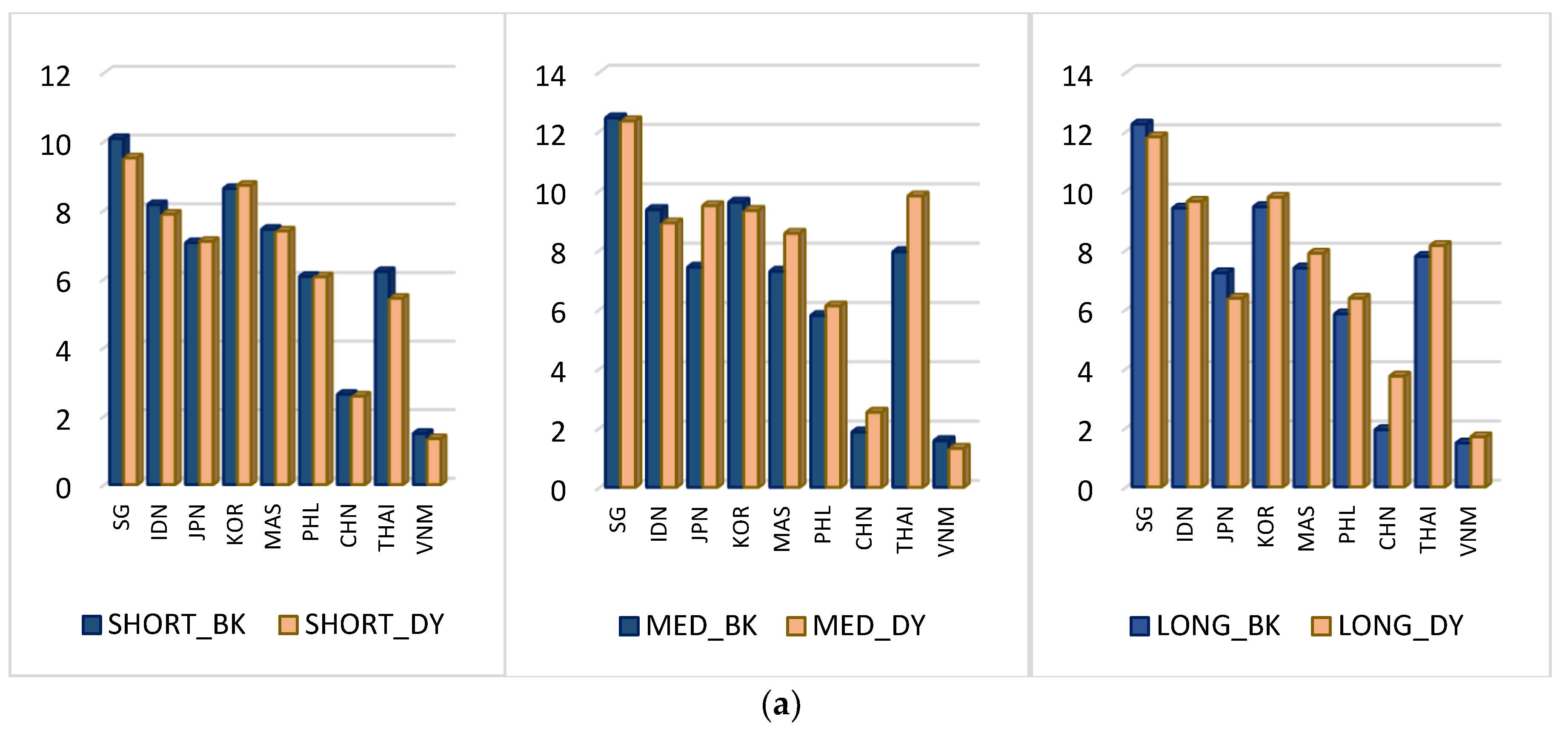
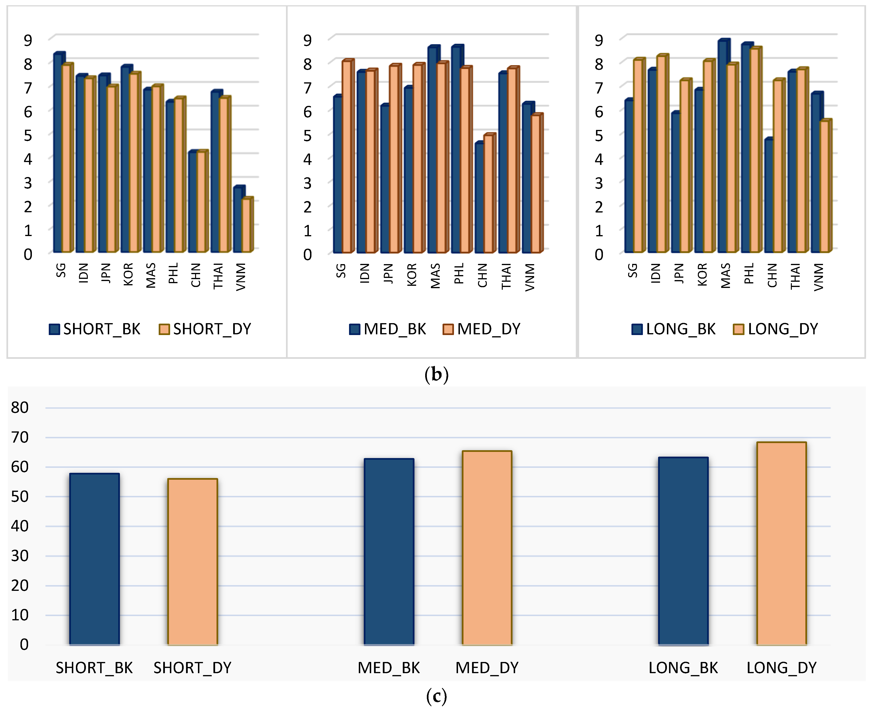
4.1. Static Connectedness

The VAR model is used to calculate volatility and return spillover over time. In constructing the volatility and spillover table, generalized variance decomposition is employed, using the DY12 methodology. We apply the generalized decomposition of variances, which allows us to measure the direction and magnitude of variances across selected markets in the time domain. Meanwhile, with the BK18 frequency domain approach, the spillover table is decomposed into three distinct frequency bands, using the Fourier transformation. Following [56], we describe the three frequency bands as follows: short-term, refers to a span of between 1 and 5 days (one week); medium-term, between 6 and 21 days (one month); and a long-term, between 22 and infinity days (one year). Consistent with [36,57], we assessed the dynamic connectedness based on a 200-day rolling window size. Furthermore, a 100-day forecast horizon is used in accordance with the BK18; albeit, the BK18 system is independent of the forecast horizon.

Table 2. Return connectedness.

Panel A. Diebold–Yilmaz Method (2012)
	SG	IDN	JPN	KOR	MAS	PHL	CHN	THAI	VNM	FROM_ABS
SG	28.81	12.34	11.51	13.95	10.65	7.24	3.74	9.84	1.91	7.91
IDN	14.20	32.92	7.22	11.06	10.58	9.85	2.46	10.32	1.40	7.45
JPN	14.56	8.02	35.95	14.91	8.10	6.28	3.26	6.68	2.25	7.12
KOR	15.44	10.62	13.19	31.73	8.93	7.28	3.27	8.14	1.39	7.59
MAS	13.27	11.75	7.83	10.02	34.70	9.31	3.03	8.78	1.30	7.26
PHL	10.59	12.14	6.99	9.42	10.52	38.28	2.06	8.24	1.76	6.86
CHN	7.99	4.76	5.47	6.25	5.39	3.16	61.36	3.72	1.90	4.29
THAI	13.07	12.00	7.06	9.81	9.00	7.60	2.24	37.69	1.53	6.92
VNM	6.24	4.37	4.63	4.05	3.60	3.39	2.13	3.53	68.06	3.55
TO	10.60	8.44	7.10	8.83	7.42	6.01	2.47	6.58	1.49	58.94
NET_ABS	2.69	0.99	−0.02	1.25	0.16	−0.85	−1.83	−0.34	−2.06
Panel B. Baruník–Křehlík method (2018)—Spillover for band 3.14 to 0.63 (roughly to 1 day to 5 days).
	SG	IDN	JPN	KOR	MAS	PHL	CHN	THAI	VNM	FROM_ABS	FROM_WTH
SG	23.43	9.99	9.38	11.31	8.69	5.8	3.25	7.79	1.51	6.41	8.33
IDN	10.67	26.02	5.58	8.23	8.2	7.74	2.03	7.79	1.09	5.7	7.41
JPN	11.31	6.42	29.6	12.14	6.6	5.3	2.83	5.01	1.84	5.72	7.43
KOR	11.99	8.45	10.69	25.76	7.12	5.83	2.75	6.05	1.11	6	7.79
MAS	9.46	8.42	5.86	7.21	26.76	6.91	2.39	6.05	0.98	5.25	6.83
PHL	7.26	8.65	4.9	6.66	7.65	30.73	1.6	5.7	1.35	4.86	6.32
CHN	5.89	3.42	4.3	4.87	4.17	2.36	49.77	2.71	1.35	3.23	4.2
THAI	9.8	8.87	5.13	7.06	6.97	5.85	1.91	29.94	1.09	5.19	6.74
VNM	3.46	2.3	2.98	2.28	2.11	2.23	1.48	1.93	50.59	2.09	2.71
TO_ABS	7.76	6.28	5.42	6.64	5.72	4.67	2.03	4.78	1.14	44.45
TO_WTH	10.08	8.16	7.05	8.63	7.44	6.07	2.63	6.21	1.49		57.76
NET ABS	1.35	0.58	−0.3	0.64	0.47	−0.19	−1.2	−0.41	−0.95
Panel C. Baruník–Křehlík method (2018)—Spillover for band 0.63 to 0.15 (roughly 6 days to 21 days).
	SG	IDN	JPN	KOR	MAS	PHL	CHN	THAI	VNM	FROM_ABS	FROM_WTH
SG	3.96	1.74	1.56	1.94	1.45	1.06	0.37	1.5	0.29	1.1	6.54
IDN	2.57	5.08	1.19	2.05	1.74	1.55	0.32	1.84	0.22	1.28	7.58
JPN	2.39	1.19	4.69	2.05	1.12	0.73	0.32	1.23	0.3	1.04	6.16
KOR	2.52	1.61	1.83	4.39	1.33	1.07	0.38	1.53	0.2	1.16	6.91
MAS	2.76	2.43	1.43	2.03	5.81	1.74	0.46	1.97	0.23	1.45	8.61
PHL	2.42	2.55	1.52	2.01	2.1	5.54	0.35	1.84	0.3	1.45	8.63
CHN	1.52	0.97	0.85	1	0.89	0.58	8.57	0.73	0.39	0.77	4.58
THAI	2.37	2.29	1.39	2	1.49	1.28	0.25	5.67	0.32	1.27	7.52
VNM	2	1.48	1.18	1.26	1.08	0.84	0.47	1.14	12.7	1.05	6.24
TO_ABS	2.06	1.58	1.22	1.59	1.24	0.98	0.32	1.31	0.25	10.57
TO_WTH	12.25	9.41	7.23	9.46	7.39	5.84	1.93	7.78	1.48		62.77
NET ABS	0.96	0.3	0.18	0.43	−0.21	−0.47	−0.45	0.04	−0.8
Panel D. Baruník–Křehlík method (2018)—Spillover for band 0.15 to 0 (roughly 21 days to infinity).
	SG	IDN	JPN	KOR	MAS	PHL	CHN	THAI	VNM	FROM_ABS	FROM_WTH
SG	1.42	0.62	0.57	0.7	0.51	0.38	0.13	0.55	0.11	0.4	6.38
IDN	0.96	1.82	0.45	0.77	0.64	0.57	0.11	0.69	0.09	0.48	7.66
JPN	0.85	0.41	1.66	0.72	0.38	0.24	0.11	0.44	0.11	0.36	5.84
KOR	0.93	0.57	0.67	1.59	0.48	0.38	0.14	0.57	0.08	0.42	6.82
MAS	1.05	0.9	0.55	0.78	2.14	0.66	0.17	0.76	0.09	0.55	8.88
PHL	0.91	0.94	0.58	0.75	0.77	2.01	0.12	0.7	0.11	0.54	8.73
CHN	0.58	0.37	0.32	0.38	0.33	0.22	3.02	0.28	0.16	0.29	4.73
THAI	0.9	0.84	0.53	0.76	0.54	0.46	0.09	2.08	0.12	0.47	7.58
VNM	0.79	0.58	0.47	0.51	0.41	0.32	0.18	0.46	4.77	0.41	6.66
TO_ABS	0.77	0.58	0.46	0.6	0.45	0.36	0.12	0.49	0.1	3.93
TO_WTH	12.45	9.36	7.42	9.61	7.28	5.79	1.86	7.94	1.57		63.29
NET ABS	0.37	0.1	0.1	0.18	−0.1	−0.18	−0.17	0.02	−0.31

Note: This table presents the return spillover results for the DY12 and BK18 approaches in Panels A and B, respectively, using the return data for each country. In Panels B–D, “FROM_ABS” is the measure of “frequency” connectedness, and “FROM_WTH” is the measure of “within” connectedness. “NET ABS” denotes the net spillover index for each market.

and

Table 3. Volatility connectedness.

Panel A. Diebold–Yilmaz method (2012)
	SG	IDN	JPN	KOR	MAS	PHL	CHN	THAI	VNM	FROM
SG	65.30	5.47	4.42	11.55	5.00	2.13	2.34	3.43	0.34	3.86
IDN	9.49	51.69	5.34	11.00	6.64	4.65	1.95	7.99	1.26	5.37
JPN	8.77	5.63	53.25	15.27	3.95	2.82	2.54	6.21	1.56	5.19
KOR	14.58	7.41	10.75	48.15	5.73	2.80	2.57	6.96	1.05	5.76
MAS	10.35	7.31	4.50	9.24	52.27	4.97	3.59	6.87	0.90	5.30
PHL	5.71	6.84	4.97	6.94	6.47	59.93	1.03	6.76	1.35	4.45
CHN	8.01	2.43	2.83	4.11	4.01	0.65	75.80	1.87	0.28	2.69
THAI	8.32	8.49	5.48	9.80	5.75	5.47	1.75	53.57	1.37	5.16
VNM	0.45	1.75	3.21	2.68	1.95	1.32	0.77	2.92	84.95	1.67
TO	7.30	5.04	4.61	7.84	4.39	2.76	1.84	4.78	0.90	39.45
NET_ABS	3.44	−0.33	−0.58	2.08	−0.92	−1.70	−0.85	−0.38	−0.77
Panel B. Baruník–Křehlík method (2018)—Spillover for band 3.14 to 0.63 (roughly to 1 day to 5 days).
	SG	IDN	JPN	KOR	MAS	PHL	CHN	THAI	VNM	FROM_ABS	FROM_WTH
SG	10.93	0.83	0.96	1.55	1.18	0.47	0.37	0.81	0.03	0.69	2.18
IDN	1.51	22.02	0.54	0.84	1.17	1	0.18	1.06	0.06	0.71	2.24
JPN	1.58	0.6	22.32	3.19	0.72	0.44	0.26	0.64	0.3	0.86	2.72
KOR	1.89	0.59	2.24	14.74	0.7	0.62	0.23	0.54	0.09	0.77	2.43
MAS	2.34	1.29	0.78	1.13	25.46	0.89	0.4	1.27	0.1	0.91	2.89
PHL	1.2	1.68	0.69	1.39	1.16	35.53	0.12	1.35	0.16	0.86	2.73
CHN	0.85	0.3	0.34	0.44	0.5	0.1	28.58	0.24	0.07	0.32	1
THAI	1.53	1.28	0.65	0.84	1.35	1.3	0.2	26.38	0.11	0.81	2.56
VNM	0.05	0.1	0.51	0.23	0.18	0.18	0.14	0.18	43.26	0.17	0.55
TO_ABS	1.22	0.74	0.75	1.07	0.77	0.56	0.21	0.68	0.1	6.09
TO_WTH	3.85	2.34	2.37	3.38	2.45	1.76	0.67	2.15	0.33		19.3
NET ABS	0.53	0.03	−0.11	0.3	−0.14	−0.3	−0.11	−0.13	−0.07
Panel C. Baruník–Křehlík method (2018)—Spillover for band 0.63 to 0.15 (roughly 6 days to 21 days).
	SG	IDN	JPN	KOR	MAS	PHL	CHN	THAI	VNM	FROM_ABS	FROM_WTH
SG	14.45	1.36	1.32	2.88	1.27	0.62	0.5	0.99	0.06	1	3.55
IDN	2.49	14.82	1.53	3.13	1.97	1.45	0.47	2.47	0.43	1.55	5.49
JPN	2.21	1.67	15.91	4.29	1.03	0.9	0.68	2.02	0.49	1.48	5.24
KOR	3.43	2.07	3.07	13.56	1.6	0.67	0.6	2.12	0.34	1.54	5.47
MAS	2.74	2.2	1.21	2.64	14.59	1.82	1.13	2.09	0.28	1.57	5.56
PHL	1.61	2.08	1.68	1.86	2.37	14.91	0.25	2.25	0.5	1.4	4.97
CHN	1.91	0.64	0.86	1.02	1.32	0.15	24.74	0.51	0.1	0.72	2.57
THAI	2.13	2.71	1.67	2.89	1.6	1.88	0.43	14.54	0.49	1.53	5.44
VNM	0.08	0.58	0.94	0.82	0.69	0.43	0.22	0.97	24.39	0.52	1.86
TO_ABS	1.85	1.48	1.37	2.17	1.32	0.88	0.48	1.49	0.3	11.32
TO_WTH	6.54	5.25	4.84	7.69	4.67	3.12	1.68	5.29	1.06		40.15
NET ABS	0.85	−0.07	−0.11	0.63	−0.25	−0.52	−0.24	−0.04	−0.22
Panel D. Baruník–Křehlík method (2018)—Spillover for band 0.15 to 0 (roughly 21 days to infinity).
	SG	IDN	JPN	KOR	MAS	PHL	CHN	THAI	VNM	FROM_ABS	FROM_WTH
SG	39.93	3.28	2.14	7.12	2.55	1.03	1.48	1.64	0.25	2.17	5.38
IDN	5.49	14.85	3.27	7.03	3.49	2.19	1.3	4.46	0.77	3.11	7.73
JPN	4.98	3.36	15.03	7.8	2.19	1.48	1.59	3.54	0.77	2.86	7.1
KOR	9.25	4.75	5.44	19.84	3.44	1.51	1.74	4.3	0.61	3.45	8.57
MAS	5.27	3.82	2.5	5.47	12.22	2.26	2.06	3.51	0.51	2.82	7.02
PHL	2.89	3.09	2.59	3.69	2.93	9.49	0.66	3.15	0.69	2.19	5.44
CHN	5.25	1.49	1.63	2.65	2.19	0.4	22.49	1.12	0.11	1.65	4.1
THAI	4.66	4.49	3.16	6.07	2.81	2.29	1.12	12.64	0.77	2.82	7
VNM	0.33	1.08	1.76	1.64	1.08	0.71	0.42	1.77	17.29	0.97	2.42
TO_ABS	4.24	2.82	2.5	4.61	2.3	1.32	1.15	2.61	0.5	22.04
TO_WTH	10.53	7.01	6.21	11.45	5.71	3.28	2.86	6.49	1.24		54.77
NET ABS	2.07	−0.29	−0.36	1.16	−0.52	−0.87	−0.5	−0.21	−0.47

Note: This table presents the volatility spillover results for the DY12 and BK18 approaches in Panels A and B, respectively, using the volatility data for each country. In Panels B–D, “FROM_ABS” is the measure of “frequency” connectedness, and “FROM_WTH” is the measure of “within” connectedness. “NET ABS” denotes the net spillover index for each market.

present the empirical results of the spillovers for return and volatility, respectively. Panel A presents the results using the DY12 method, while Panels B–D provide estimates for the BK18 method for the three frequency bands. The cross-market spillover effect can be found from row to column, indicating the directional spillovers from market i-th to the j-th market and vice versa. The last number in the last column in Panel A gives the total spillover from all other variables. Likewise, the last number in the second last column in Panels B–D, “FROM_ABS”, provides the total frequency connectedness for three frequency bands, where summing these three parts equals the total connectedness index of “FROM” in Panel A. “FROM_WTH” presents the unweighted connectedness from the variable that is within its respective band, rather than outside. Moreover, the “TO” in Panel A and “TO_ABS” in Panels B–D indicate the spillover to all variables, and “TO_WTH” is the unweighted connectedness to other variables that are within its frequency band. Last, “NET_ABS” calculates the difference between the “TO_ABS” row and “FROM_ABS” column, whereby a positive (negative) value indicates transmitter (receiver) of return and volatility to (from) other markets.

We first present the time domain results using the DY12 method in Panel A, then follows the frequency domain results for the short-, medium-, and long-term using the BK18 method in Panels B, C, and D, respectively. As shown in Table 2, the total connectedness in returns reaches 58.94%, and the total connectedness in volatility stands at 39.45% in Table 3. This indicates that the stock market returns for ASEAN+3 economies have a stronger connectedness than in volatilities. In Panels B–D, we find the frequency connectedness for returns in the short-, medium-, and long-term are 44.45%, 10.57%, 3.93%, respectively, which means that the return spillover emanating from one market transmitted to other markets produces only short-term consequences. Moreover, based on the volatility spillover results in Table 3, the frequency spillover (FROM_ABS) in the short-, medium-, and long-term are 6.09%, 11.32%, and 22.04%, respectively. Nonetheless, unlike the return spillover, the volatility spillover from one market transmits to other markets, sparked off by impacts that run for a long period of time. Baruník and Křehlík [34] opine that the opposing spillover effects between asset returns and volatilities in the frequency domain are due to the construction of the series themselves. Volatility takes longer to transmit from one market to another because it is induced after a return. Thus, the impact of a shock in a system is transmitted quickly to asset returns, first, before being diffused to volatilities. This explains the finding of [36], in which shock effects were merely temporary and short-lived, for only a few days, when investors had not reacted to any speculations induced by market news. This also throws a light onto why volatility shocks last longer when the relationship is formed at lower frequencies.

Table 2 also reveals that in the time domain, the largest transmitters and receivers of spillovers are Singapore (10.6%, 7.91%) and Korea (8.83%, 7.59%). The Singapore stock market is the largest transmitter of return spillover to other markets, followed by South Korea and Indonesia. Vietnam, China, and the Philippines are the highest receivers of return spillover. With respect to the total spillovers in the short-term frequency, a high level of spillovers is observed amongst Singapore, Korea, and Japan markets. In the medium-term and long-term frequency, Singapore still stands as the top transmitter of stock returns, and Vietnam is the top receiver. Likewise, Table 3 shows that Singapore contribute the most to volatility spillovers in all frequencies; short-term (1.22%), medium-term (1.85%), and long-term (4.24%), followed by South Korea (1.07% for short term, 2.17% for medium term, 4.61% for long term). Both Table 2 and Table 3 indicate that Singapore is a significant contributor of spillover to ASEAN countries, mainly Malaysia, Indonesia, the Philippines, and Thailand. Our evidence is consistent with [58], who also documented a strong stock market integration between Singapore and ASEAN countries during the GFC period. Our findings are also comparable to [40], who emphasize the role of China as the highest net receiver of shocks, while Singapore contributes the most spillovers among the APT countries.

The markets that transmit the lowest level of volatility shocks to the others are China (0.21%, 0.48%, 1.15%) and Vietnam (0.1%, 0.3%, 0.5%), respectively. Meanwhile, the markets which received the highest level of volatility, albeit for just a short period, were Malaysia (0.91%), the Philippines (0.86%), and Japan (0.86%). Throughout the whole observation, volatility spillovers occurred at a higher rate for the long-term spillovers from one market to another, as opposed to the spillovers that occurred in the medium- and long-term. This finding is consistent with [59], who found that volatility spillovers are higher for the long periods when compared to short- and medium-periods, factoring the dynamic connectedness between several important financial variables and renewable stock markets. Our results show that the shocks to ASEAN+3 are slowly absorbed by the markets (within a week) and traders build their response gradually over the long term. In contrast, the highest receivers of volatility in the long run are South Korea (3.45%), Indonesia (3.11%), and Japan (2.86%). This finding indicates that when ASEAN+3 financial markets are exposed to external shocks, these markets tend to be the slowest to adjust. In other words, investors react slowly when facing market shocks, giving ample time for the real sector to adapt; a finding similar to that of BRICS economies in [60].

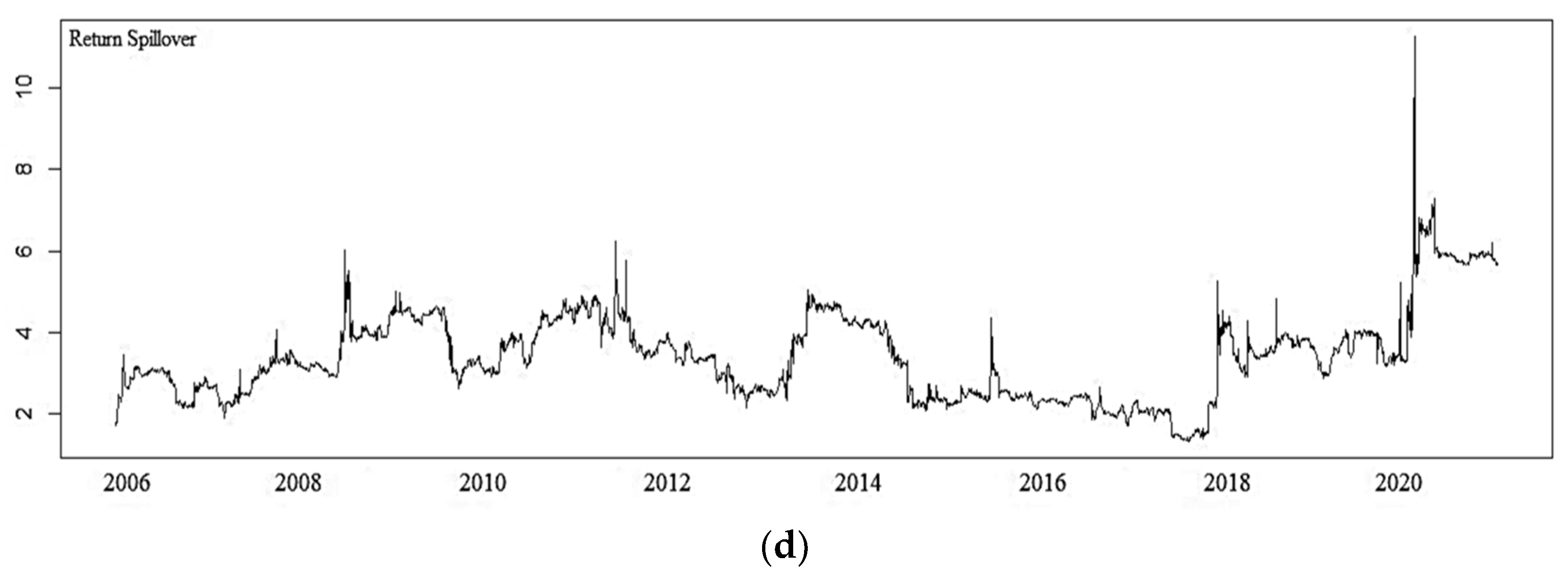
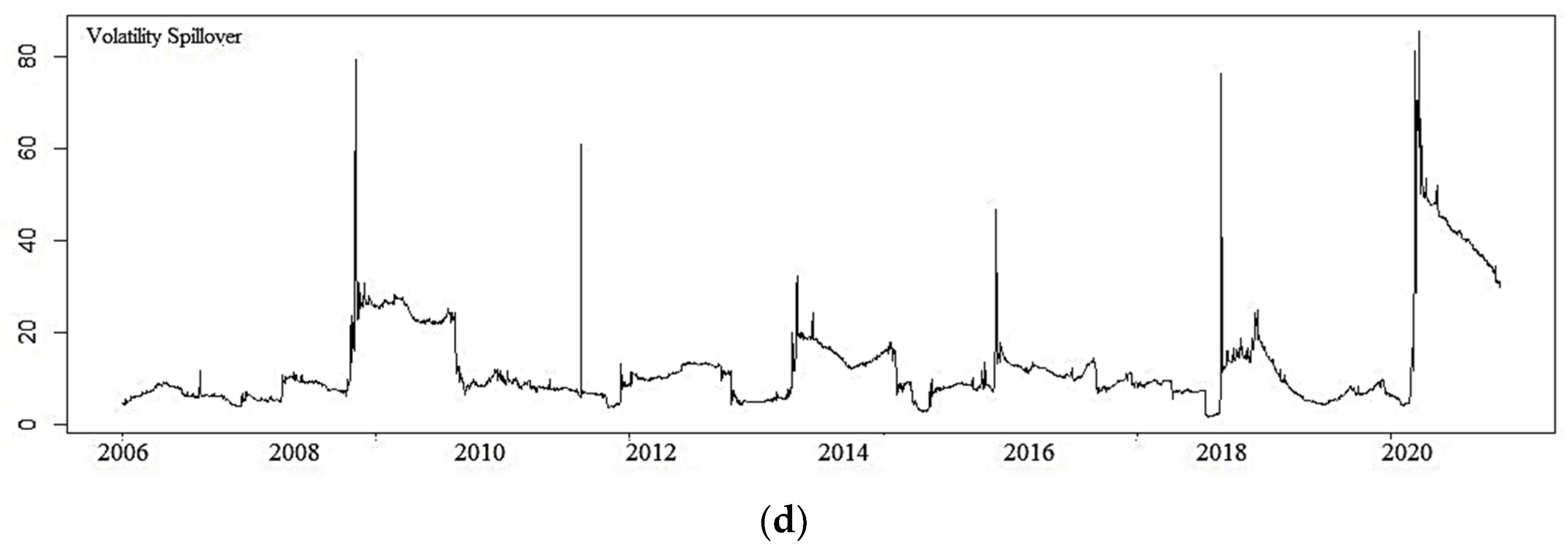
4.2. Dynamic Rolling Connectedness

To examine the return and volatility spillovers over time, a three-periodic trajectory was mapped out. Figure 3 and Figure 4 illustrate these three trajectories as short-, intermediate-, and long-term, by plotting the daily log-returns (volatility) of total spillovers in the time and frequency domains. A 200-day rolling window size was plotted, with a 100-day forecast horizon. Meanwhile, in the time domain, as exhibited in Panel (a), three key crises—the 2008–2009 global financial crisis, the downturn in China’s growth in 2016, and the ongoing COVID-19 pandemic—are selected as the driving factors determining the return and volatility spillovers. To be exact, we can very well observe that the total spillover of returns (volatility) increased, and subsequently it oscillated around 40–60% (20–40%), following the global financial crisis in 2008. However, the COVID-19 pandemic in 2020 had the effect of pushing the total return (volatility) connectedness above 75% (80%). In other words, volatility connectedness is more vulnerable to extreme crises in the time domain.

The graphical evidence for frequency connectedness from Panels (b) to (d) of Figure 3 and Figure 4 indicates that short-term return spillovers dominate the medium- and long-term spillovers, whereas volatility spillovers are evidently more distinct in the long-term rather than in the short- and medium-term, consistent with Table 2 and Table 3. In contrast to Figure 3, the total volatility spillover in Figure 4 fluctuates dramatically and has multiple spike points. These sharp fluctuations are most notable in the short-term frequency band i.e., Panel (b), whereby high spillovers are observed around 2008–2009, during GFC; around 2015, which correlates with the rapid fall in oil prices; around 2017, consequent to the increase of the Federal Reserve’s interest rate in the United States; and around 2018, following trade uncertainty between China and the United States. Apart from the year 2020, Panel (d) for the long-term frequency band, exhibits a relatively smooth pattern, fluctuating around 2–6% for return and around 4% to 20% for volatilities. From 2020 onwards, it is evident that COVID-19 exerted a significant impact on the volatility spillover of ASEAN+3 stock markets, reaching above 80% and exceeding the impact of the 2008 GFC.

Overall, the results from the dynamic moving-window analysis reveal that spillover in volatilities primarily happens over the long run, followed by the medium term and the short term. This, however, is not the case for returns spillovers in the frequency-based domain. In fact, the assertion that the shocks which COVID-19 has had on returns and volatilities are significantly higher than any of the previous global incidents is reiterated here. Our results are in full agreement with [42], who documented a similar impact of COVID-19 on commodity and stock exchanges.

4.3. Robustness

A further step in this paper is to apply a wavelet-based decomposed series in the DY12 framework and determine whether we could replicate the within connectedness index of the BK18 method as a robustness check. Since the within connectedness index of BK18 is regarded as a pure unweighted frequency connectedness index, the GFEVD methodology in DY12 may be utilized to replicate the within index of BK18 from data decomposed according to the time–frequency domain. Accordingly, we decomposed our return and volatilities series using maximal overlap discrete wavelet transform (MODWT). As specified by [61], MODWT is able to process all sample sizes, including non-dyadic lengths with an improved asymptotically efficiency (see also [37]).

Next, we used the DY12 method to estimate the spillover index and plot the connectedness index of returns and volatilities in Figure 5 and Figure 6, respectively. To facilitate analysis, we performed side-by-side comparisons of the BK18 and DY12 methods, assessing the “To”, “From”, and “Total” connectedness indexes across three separate Panels (a, b, and c).

Overall, as exhibited in Figure 5 and Figure 6, we observed a highly comparable index of connectedness calculated using the DY12 method from wavelet-based series and the within spillover index from the BK18 method. Specifically, the “To”, “From”, and “Total” spillovers across the three frequency domains in returns and volatilities only differed by a few percentage points between the two methods. Our results show that the unweighted within spillover index of BK18 may be reproduced with a high level of similarity using the time-domain method of DY12. This exercise mainly serves two purposes: First, is to confirm the robustness of our frequency-based indexes, and second is to expand the use of the wavelet-based method in the literature of dynamic connectedness in asset markets.

5. Conclusions

In this paper, the effect of the COVID-19 pandemic on directional spillovers amongst nine Asian countries, known as the ASEAN+3, was examined. For our empirical analysis, we used daily data ranging from 10 May 2005 to 24 February 2021. Our study is the first to examine the return and volatility spillovers among ASEAN+3 stock markets from time-domain (DY12) and frequency-domain (BK18) perspectives. We demonstrated that the COVID-19 pandemic has had a bigger impact on the return and volatilities of ASEAN+3 stock markets than previous economic turmoil, affirming the findings of [11]. Using a frequency-domain methodology, we found evidence that return spillovers mostly occur in the short-term, while volatility connectedness is more pronounced in the long-term. Most of the spikes in short-term spillovers correspond to global events, namely the 2008 GFC, 2016 Chinese economic downturn, and the ongoing COVID-19 epidemic. Long-term spillovers are less pronounced, except from 2020 onwards, suggesting a long-lasting effect of the current pandemic is exerting on the system. We also recognized that the Singapore stock market acts primarily as the top transmitter in returns and volatilities for many ASEAN countries, suggesting that ASEAN countries are increasingly interconnected, especially during economic crisis. We also demonstrated that it is possible to reproduce the frequency domain spillovers of BK18 from the DY12 methodology. Using a series decomposed with the wavelet procedure, we found that the total spillover indices for short-, medium-, and long-term frequencies computed with the DY12 approach are comparable to the within connectedness indices of BK18.

Our results have several important implications for investors and policy makers, especially in Asian countries. Investors should consider short- and long-term transmission of volatility asymmetry. Equity investors may generate more diversification benefits, especially over a one-week period, than generated merely for longer time periods, by incorporating assets derived from emerging ASEAN markets, namely Vietnam, Malaysia, and the Philippines. Against this backdrop, portfolio managers who factor in frequency decomposition in their management will substantially improve their knowledge diffusion, as well as heighten their cognizance of how volatility spillovers occur between markets. Furthermore, there should be constant monitoring of the interrelationships between asset markets in ASEAN+3 economies, so that policymakers are more informed of the spillover effects caused by financial instability, especially regarding the ongoing impacts of the COVID-19 pandemic. They should, therefore, develop policies to track stock market instability that can help companies boost their cash flows and increase shareholders’ wealth. This would reduce drawdowns and risk exposures in the financial system when a stock market is confronted with a declining trajectory that may be fueled by an extreme crisis.

References

1. Dias, R.; Da Silva, J.V.; Dionísio, A. Financial markets of the LAC region: Does the crisis influence the financial integration? Int. Rev. Financ. Anal. 2019, 63, 160–173. [Google Scholar] [CrossRef]
2. Jondeau, E.; Rockinger, M. The Copula-GARCH model of conditional dependencies: An international stock market application. J. Int. Money Financ. 2006, 25, 827–853. [Google Scholar] [CrossRef] [Green Version]
3. Mokni, K.; Mansouri, F. Conditional dependence between international stock markets: A long-memory GARCH copula model approach. J. Multinatl. Financ. Manag. 2017, 42–43, 116–131. [Google Scholar] [CrossRef]
4. Azimili, A. The impact of COVID-19 on the degree of dependence and structure of risk return relationship: A quintile regression approach. Financ. Res. Lett. 2020, 36, 101648. [Google Scholar] [CrossRef] [PubMed]
5. Cepoi, C.O. Asymmetric dependence between stock market returns and news during COVID-19 financial turmoil. Financ. Res. Lett. 2020, 36, 101658. [Google Scholar] [CrossRef] [PubMed]
6. Topcu, M.; Gulal, O.S. The impact of COVID-19 on emerging stock markets. Financ. Res. Lett. 2020, 36, 101691. [Google Scholar] [CrossRef]
7. Sharif, A.; Aloui, C.; Yarovaya, L. COVID-19 pandemic, oil prices, stock market, geopolitical risk and policy uncertainty nexus in the U.S. economy: Fresh evidence from the wavelet-based approach. Int. Rev. Financ. Anal. 2020, 70, 101496. [Google Scholar] [CrossRef]
8. Yarovaya, L.; Ahmed, H.E.; Shawkat, M.H. Searching for Safe Havens during the COVID-19 Pandemic: Determinants of Spillovers between Islamic and Conventional Financial Markets. 2020. Available online: https://papers.ssrn.com/sol3/papers.cfm?abstract_id=3634114 (accessed on 15 July 2021).
9. Anh, D.L.T.; Gan, C. The impact of the COVID-19 lockdown on stock market performance: Evidence from Vietnam. J. Econ. Stud. 2021, 48, 836–851. [Google Scholar] [CrossRef]
10. Kamaludin, K.; Sundarasen, S.; Ibrahim, I. COVID-19, Dow Jones and equity market movement in ASEAN-5 countries: Evidence from wavelet analyses. Heliyon 2021, 7, e05851. [Google Scholar] [CrossRef]
11. Baker, S.R.; Bloom, N.; Davis, S.J.; Kost, K.; Sammon, M.; Viratyosin, T. The unprecedented stock market reaction to COVID-19. Rev. Asset Pricing Stud. 2020, 10, 742–758. [Google Scholar] [CrossRef]
12. Ammy-Driss, A.; Garcin, M. Efficiency of the financial markets during the COVID-19 crisis: Time-varying parameters of fractional stable dynamics. arXiv 2020, arXiv:2007.10727. [Google Scholar]
13. Hung, N.T. Dynamic spillover effects between oil prices and stock markets: New evidence from pre and during COVID-19 outbreak. AIMS Energy 2020, 8, 819–834. [Google Scholar] [CrossRef]
14. McKibbin, W.J.; Vines, D. Global macroeconomic cooperation in response to the COVID-19 pandemic: A roadmap for the G20 and the IMF. Oxf. Rev. Econ. Policy 2020, 36, S297–S337. [Google Scholar] [CrossRef]
15. Ali, M.; Nafis, A.; Rizvi, S.A.R. Coronavirus (COVID-19)—An epidemic or pandemic for financial markets. J. Behav. Exp. Financ. 2020, 27, 100341. [Google Scholar] [CrossRef] [PubMed]
16. Barro, R.J.; José, F.U.; Joanna, W. The Coronavirus and the Great Influenza Pandemic: Lessons from the “Spanish flu” for the Coronavirus’s Potential Effects on Mortality and Economic Activity; NBER Working Paper No. 26866; National Bureau of Economic Research: Cambridge, MA, USA, 2020. [Google Scholar]
17. Zhang, D.; Min, H.; Qiang, J. Financial markets under the global pandemic of COVID-19. Financ. Res. Lett. 2020, 36, 101528. [Google Scholar] [CrossRef] [PubMed]
18. King, M.; Sentana, E.; Wadhwani, S. Volatility and links between national stock markets. Econometrica 1994, 62, 901–933. [Google Scholar] [CrossRef]
19. Forbes, K.J.; Rigobon, R. No contagion, only interdependence: Measuring stock market comovements. J. Financ. 2002, 57, 223–261. [Google Scholar] [CrossRef]
20. Berben, R.P.; Jansen, W.J. Comovement in international equity markets: A sectoral view. J. Int. Money Financ. 2005, 24, 832–857. [Google Scholar] [CrossRef] [Green Version]
21. Bartram, S.M.; Taylor, S.J.; Wang, Y.-H. The Euro and European financial market dependence. J. Bank. Financ. 2007, 31, 1461–1481. [Google Scholar] [CrossRef]
22. Kasa, K. Common stochastic trends in international stock markets. J. Monet. Econ. 1992, 29, 95–124. [Google Scholar] [CrossRef]
23. Manopimoke, P.; Prukumpai, S.; Sethapramote, Y. Dynamic Connectedness in Emerging Asian Equity Markets. In Banking and Finance Issues in Emerging Markets; Barnett, W.A., Sergi, B.S., Eds.; Emerald Publishing Limited: Bingley, UK, 2018; pp. 51–84. [Google Scholar]
24. Jiang, Y.; Yu, M.; Hashmi, S.M. The financial crisis and co-movement of global stock markets—A case of six major economies. Sustainability 2017, 9, 260. [Google Scholar] [CrossRef] [Green Version]
25. Madaleno, M.; Pinho, C. International stock market indices comovements: A new look. Int. J. Financ. Econ. 2012, 17, 89–102. [Google Scholar] [CrossRef]
26. Diebold, F.X.; Yilmaz, K. Measuring financial asset return and volatility spillovers, with application to global equity markets. Econ. J. 2009, 119, 158–171. [Google Scholar] [CrossRef] [Green Version]
27. Diebold, F.X.; Yilmaz, K. Better to give than to receive: Predictive directional measurement of volatility spillovers. Int. J. Forecast. 2012, 28, 57–66. [Google Scholar] [CrossRef] [Green Version]
28. Diebold, F.X.; Yilmaz, K. On the network topology of variance decompositions: Measuring the connectedness of financial firms. J. Econom. 2014, 182, 119–134. [Google Scholar] [CrossRef] [Green Version]
29. Maghyereh, A.I.; Awartani, B.; Al Hilu, K. Dynamic transmissions between the US and equity markets in the MENA countries: New evidence from pre-and post-global financial crisis. Q. Rev. Econ. Financ. 2015, 56, 123–138. [Google Scholar] [CrossRef] [Green Version]
30. Mensi, W.; Boubaker, F.Z.; Al-Yahyaee, K.H.; Kang, S.H. Dynamic volatility spillovers and connectedness between global, regional, and GIPSI stock markets. Financ. Res. Lett. 2018, 25, 230–238. [Google Scholar] [CrossRef]
31. Kang, S.H.; Uddin, G.S.; Troster, V.; Yoon, S.-M. Directional spillover effects between ASEAN and world stock markets. J. Multinatl. Financ. Manag. 2019, 52, 100592. [Google Scholar] [CrossRef]
32. Koop, G.; Pesaran, M.H.; Potter, S.M. Impulse response analysis in non-linear multivariate models. J. Econom. 1996, 74, 119–147. [Google Scholar] [CrossRef]
33. Pesaran, M.H.; Shin, Y. Generalized impulse response analysis in linear multivariate models. Econ. Lett. 1998, 58, 17–29. [Google Scholar] [CrossRef]
34. Baruník, J.; Křehlík, T. Measuring the frequency dynamics of financial connectedness and systemic risk. J. Financ. Econom. 2018, 16, 271–296. [Google Scholar] [CrossRef]
35. Tiwari, A.K.; Cunado, J.; Gupta, R.; Wohar, M.E. Volatility spillovers across global asset classes: Evidence from time and frequency domains. Q. Rev. Econ. Financ. 2018, 70, 194–202. [Google Scholar] [CrossRef]
36. Ferrer, R.; Shahzad, S.J.H.; López, R.; Jareño, F. Time and frequency dynamics of connectedness between renewable energy stocks and crude oil prices. Energy Econ. 2018, 76, 1–20. [Google Scholar] [CrossRef]
37. Mensi, W.; Hernandez, J.A.; Yoon, S.M.; Vo, X.V.; Kang, S.H. Spillovers and connectedness between major precious metals and major currency markets: The role of frequency factor. Int. Rev. Financ. Anal. 2021, 74, 101672. [Google Scholar] [CrossRef]
38. Liao, T.G.; Diaz, J.F. Real GDP growth rates of the ASEAN region: Evidence of spillovers and asymmetric volatility effects. Labu. Bull. Int. Bus. Financ. 2019, 18, 39–61. [Google Scholar]
39. Giang, N.K.; Yap, L. Vietnam Is Asia’s Best Stock Market Performer in May. 2020. Available online: https://www.bloomberg.com/news/articles/2020-05-27/inside-asia-s-best-stock-rally-in-may-vietnam-markets-primer (accessed on 3 March 2021).
40. Wu, F. Stock market integration in East and South East Asia: The role of global factor. Int. Rev. Financ. Anal. 2020, 67, 101406. [Google Scholar] [CrossRef]
41. Karkowska, R.; Urjasz, S. Connectedness structures of sovereign bond markets in Central and Eastern Europe. Int. Rev. Financ. Anal. 2021, 74, 101644. [Google Scholar] [CrossRef]
42. Zhang, W.; Hamori, S. Crude oil market and stock markets during the COVID-19 pandemic: Evidence from the US, Japan, and Germany. Int. Rev. Financ. Anal. 2021, 74, 101702. [Google Scholar] [CrossRef]
43. The Economist. Spread and Stutter. 2020. Available online: https://www.economist.com/finance-and-economics/2020/02/27/markets-wake-up-with-a-jolt-to-the-implications-of-covid-19 (accessed on 4 March 2021).
44. Aslam, F.; Saqib, A.; Duc, K.N.; Khurrum, S.M.; Maaz, K. On the efficiency of foreign exchange markets in times of the COVID-19 pandemic. Technol. Forecast. Soc. Chang. 2020, 161, 120261. [Google Scholar] [CrossRef]
45. Lin, W.-L.; Engle, R.F.; Ito, T. Do bulls and bears move across borders? International transmission of stock returns and volatility. Rev. Financ. Stud. 1994, 7, 507–538. [Google Scholar] [CrossRef]
46. Onali, E. COVID-19 and Stock Market Volatility. 2020. Available online: https://ssrn.com/abstract=3571453 (accessed on 24 April 2021).
47. Al-Awadhi, A.M.; Al-Saifi, K.; Al-Awadhi, A.; Alhammadi, S. Death and contagious infectious diseases: Impact of the COVID-19 virus on stock market returns. J. Behav. Exp. Financ. 2020, 27, 100326. [Google Scholar] [CrossRef] [PubMed]
48. Papadamous, S.; Fassas, A.; Kenourgios, D.; Dimitrious, D. Direct and Indirect Effects of COVID-19 Pandemic on Implied Stock Market Volatility: Evidence from Panel Data Analysis. MPRA Paper 100020. 2020. Available online: https://mpra.ub.uni-muenchen.de/100020/1/MPRA_paper_100020.pdf (accessed on 21 May 2021).
49. Kwapień, J.; Wątorek, M.; Drożdż, S. Cryptocurrency market consolidation in 2020–2021. Entropy 2021, 23, 1674. [Google Scholar] [CrossRef] [PubMed]
50. ASEAN. Overview of ASEAN Plus Three Cooperation, ASEAN Secretariat Information Paper. April 2020. Available online: https://asean.org/storage/2016/01/APT-Overview-Paper-24-Apr-2020.pdf (accessed on 31 December 2020).
51. Dias, R.; Pardal, P.; Teixeira, N.; Machoca, V. Financial market integration of ASEAN-5 with China. Littera Scr. 2020, 13, 46–63. [Google Scholar] [CrossRef]
52. Pradhan, R.P.; Arvin, B.M.; Norman, N.R.; Nair, M.; Hall, J.H. Insurance penetration and economic growth nexus: Cross-country evidence from ASEAN. Res. Int. Bus. Financ. 2016, 36, 447–458. [Google Scholar] [CrossRef]
53. Gulzar, S.; Kayani, G.M.; Feng, H.X.; Ayub, U.; Rafique, A. Financial cointegration and spillover effect of global financial crisis: A study of emerging Asian financial markets. Econ. Res.-Ekon. Istraživanja 2019, 32, 217–318. [Google Scholar] [CrossRef] [Green Version]
54. Daubechies, I. Orthonormal bases of compactly supported wavelets. Commun. Pure Appl. Math. 1988, 41, 909–996. [Google Scholar] [CrossRef] [Green Version]
55. Daubechies, I. Ten Lectures on Wavelets; Society for Industrial and Applied Mathematics: Philadelphia, PA, USA, 1992. [Google Scholar]
56. Toyoshima, Y.; Hamori, S. Measuring the time-frequency dynamics of return and volatility connectedness in global crude oil markets. Energies 2018, 11, 2893. [Google Scholar] [CrossRef] [Green Version]
57. Lovcha, Y.; Perez-Laborda, A. Dynamic frequency connectedness between oil and natural gas volatilities. Econ. Model. 2020, 84, 181–189. [Google Scholar] [CrossRef]
58. Wahyudi, S.; Najmudin, L.R.; Rachmawati, R. Assessing the contagion effect on herding behaviour under segmented and integrated stock markets circumstances in the USA, China, and ASEAN-5. Econ. Ann.-XXI 2018, 169, 15–20. [Google Scholar] [CrossRef] [Green Version]
59. Liu, T.; Hamori, S. Spillovers to renewable energy stocks in the US and Europe: Are they different? Energies 2020, 13, 3162. [Google Scholar] [CrossRef]
60. Wang, X.; Wang, Y. Volatility spillovers between crude oil and Chinese sectoral equity markets: Evidence from a frequency dynamics perspective. Energy Econ. 2019, 80, 995–1009. [Google Scholar] [CrossRef]
61. Maghyereh, A.I.; Abdoh, H.; Awartani, B. Connectedness and hedging between gold and Islamic securities: A new evidence from time-frequency domain approaches. Pac. Basin Financ. J. 2019, 54, 13–28. [Google Scholar] [CrossRef]
Figure 1. Dynamics of stock market returns for ASEAN+3.
Mathematics 10 01417 g001
Figure 2. Heat map of the correlation. This figure shows a visual correlation matrix across asset returns for ASEAN+3. The magnitude of correlations is shown by the color intensity of the shaded boxes. Blue denotes positive correlation, while red denotes negative correlation. Please refer to Table 1 for abbreviations of ASEAN+3 countries. All correlations are significant at a 1% level.
Mathematics 10 01417 g002
Figure 3. Distribution plots and pairwise correlations of asset returns for ASEAN+3. Return spillover based on the DY12 and BK18 methods: (a) Connectedness on asset return using DY12; (b) BK18 frequency domain for short-term (1 day to 5 days); (c) BK18 frequency domain for medium-term (from 6 days to 22 days); (d) BK18 frequency domain for long-term (22 days to infinity). The dynamic volatility connectedness is measured using a 200-day rolling window and a forecast horizon of H = 100 days.
Mathematics 10 01417 g003aMathematics 10 01417 g003b
Figure 4. Volatility spillover based on the DY12 and BK18 methods: (a) Connectedness on asset volatility using DY12; (b) BK18 frequency domain for short-term (1 day to 5 days); (c) BK18 frequency domain for medium-term (from 6 days to 22 days); (d) BK18 frequency domain for long-term (22 days to infinity). The dynamic volatility connectedness is measured using a 200-day rolling window and a forecast horizon of H = 100 days.
Mathematics 10 01417 g004aMathematics 10 01417 g004b
Figure 5. Side-by-side comparison of return spillover based on BK18 and wavelet-based DY12 methods: (a) Return To; (b) Return From; (c) Total Return. The y-axis denotes return spillovers. The x-axis description is as follows: Short_BK, Med_BK, and Long_BK are within spillover indexes calculated using the BK18 method for the short-, medium-, and long-term. Short_WAV, Med_WAV, and Long_WAV are spillover indexes calculated using the DY12 method from wavelet-based series for the short-, medium-, and long-term. Total return is the total return spillover between the two mentioned methods.
Mathematics 10 01417 g005aMathematics 10 01417 g005b
Figure 6. Side-by-side comparison of volatility spillover based on the BK18 and wavelet-based DY12 methods: (a) Volatility To; (b) Volatility From; (c) Total Volatility. The y-axis denotes volatility spillovers. The x-axis description is as follows: Short_BK, Med_BK, and Long_BK are within spillover indexes calculated using the BK18 method for the short-, medium-, and long-term. Short_WAV, Med_WAV, and Long_WAV are spillover indexes calculated using the DY12 method from wavelet-based series for the short-, medium-, and long-term. Total volatility is the total volatility spillover between the two mentioned methods.
Mathematics 10 01417 g006aMathematics 10 01417 g006b