On the Autocorrelation Function of 1/f Noises

Abstract

The outputs of many real-world complex dynamical systems are time series characterized by power-law correlations and fractal properties. The first proposed model for such time series comprised fractional Gaussian noise (fGn), defined by an autocorrelation function $C\left(k\right)$ with asymptotic power-law behavior, and a complicated power spectrum $S\left(f\right)$ with power-law behavior in the small frequency region linked to the power-law behavior of $C\left(k\right)$. This connection suggested the use of simpler models for power-law correlated time series: time series with power spectra of the form $S\left(f\right)\sim 1/f^{\beta }$, i.e., with power-law behavior in the entire frequency range and not only near $f=0$ as fGn. This type of time series, known as $1/f^{\beta }$ noises or simply $1/f$ noises, can be simulated using the Fourier filtering method and has become a standard model for power-law correlated time series with a wide range of applications. However, despite the simplicity of the power spectrum of $1/f^{\beta }$ noises and of the known relationship between the power-law exponents of $S\left(f\right)$ and $C\left(k\right)$, to our knowledge, an explicit expression of $C\left(k\right)$ for $1/f^{\beta }$ noises has not been previously published. In this work, we provide an analytical derivation of $C\left(k\right)$ for $1/f^{\beta }$ noises, and we show the validity of our results by comparing them with the numerical results obtained from synthetically generated $1/f^{\beta }$ time series. We also present two applications of our results: First, we compare the autocorrelation functions of fGn and $1/f^{\beta }$ noises that, despite exhibiting similar power-law behavior, present some clear differences for anticorrelated cases. Secondly, we obtain the exact analytical expression of the Fluctuation Analysis algorithm when applied to $1/f^{\beta }$ noises.

1. Introduction

The information available from many complex dynamical systems typically consists of observable output time series, which presents characteristics inherited from underlying dynamics. In particular, the most remarkable feature is the presence of long-range power-law correlations in such time series as a signature of fractal properties and the lack of characteristic spatial or time scales in the system. Such power-law correlations are practically ubiquitous, and since the discovery of the Hurst effect in the Nile river [1], they have been found in a great diversity of natural and artificial systems: stock market activity [2], physiology (heartbeat dynamics [3,4,5], respiration [6], brain activity [7], postural control [8,9], etc.), DNA sequences [10], cellular automaton [11], meteorology [12], geophysics [13], and many others.

As a consequence of the abundance of these time series, it is convenient to create mathematical models able to reproduce such power-law correlations and to generate synthetic time series with properties mimicking those of real-world time series. Very likely, the first model characterized by fractal properties and power-law correlations are the well-known fractional Gaussian noises (fGns) proposed by Mandelbrot and Van Ness [14]. FGns are provided by the increments of fractional Brownian motions (typically used to describe anomalous diffusion), and they are fully characterized by the following autocorrelation function:

$$C\left(k\right)={\displaystyle \frac{{(k+1)}^{2H}-2k^{2H}+{(k-1)}^{2H}}{2}}$$

(1)

where H is the Hurst exponent defining the process, with $H\in (0,1)$ used to ensure stationarity. In the limit of large values of lag k, $C\left(k\right)$ behaves as a power-law.

$$C\left(k\right)\simeq \frac{H(2H-1)}{k^{2-2H}}$$

(2)

This is the reason why these noises are termed as power-law correlated. Case $H=1/2$ corresponds to the absence of correlations (white noise) for which $C\left(k\right)=0$. For $H>1/2$, the correlations are positive and are stronger as H increases, while the noise is power-law anticorrelated for $H<1/2$. Moreover, for $H>1/2$, the sum ${\sum }_{k=1}^{\infty }C\left(k\right)$ diverges, and the corresponding noise is known as a long-range correlated.

FGns can be computationally generated using different methods, such as the one proposed by Davies and Harte [15]. In this technique, Equation (1) is used to compute N values of $C\left(k\right)$ from $k=0$ to $N-1$, which are then conveniently arranged in a periodic manner prior to numerically calculating the Fourier transform to obtain the power spectrum $S\left(f\right)$ according to the Wiener–Khinchin theorem. $S\left(f\right)$ is later used to generate a signal in the frequency domain with random Fourier phases. This signal is Fourier-transformed back into the time domain to obtain a particular realization of fGn with N data points.

Other techniques detailed by Dieker and Mandjes in [16] use the corresponding power spectrum $S\left(f\right)$ as the starting point for the generation of fGn:

$$S\left(f\right)=2sin\left(\pi H\right)\Gamma (2H+1)(1-cos\left(2\pi f\right))\left[{\left(2\pi f\right)}^{-2H-1}+B(f,H)\right],$$

(3)

with the function $B(f,H)$ defined as:

$$B(f,H)=\frac{{\sum }_{j=1}^{\infty }{(j+f)}^{-2H-1}+{(j-f)}^{-2H-1}}{{\left(2\pi \right)}^{1+2H}},$$

(4)

and with the frequency f in range $-1/2<f<1/2$. Using this (complicated) power-spectrum, the aim is to construct a signal that is a frequency domain and to transform it back to the time domain for obtaining a final time series of fGn type. We remark that, in the limit of small frequencies (large scales) near $f=0$, the fGn power spectrum (3) behaves as follows:

$$S\left(f\right)\sim \frac{1}{f^{2H-1}}\equiv \frac{1}{f^{\beta }},$$

(5)

where we have defined exponent $\beta$ of $S\left(f\right)$ as $\beta =2H-1$ with $\beta \in (-1,1)$, and then in terms of the $\beta$ exponent, the power-law behavior of $C\left(k\right)$ is $C\left(k\right)\sim k^{1-\beta }$. In this manner, the large scale power-law behavior of $C\left(k\right)$ in Equation (2) is linked to the power-law behavior of $S\left(f\right)$ in the small f region.

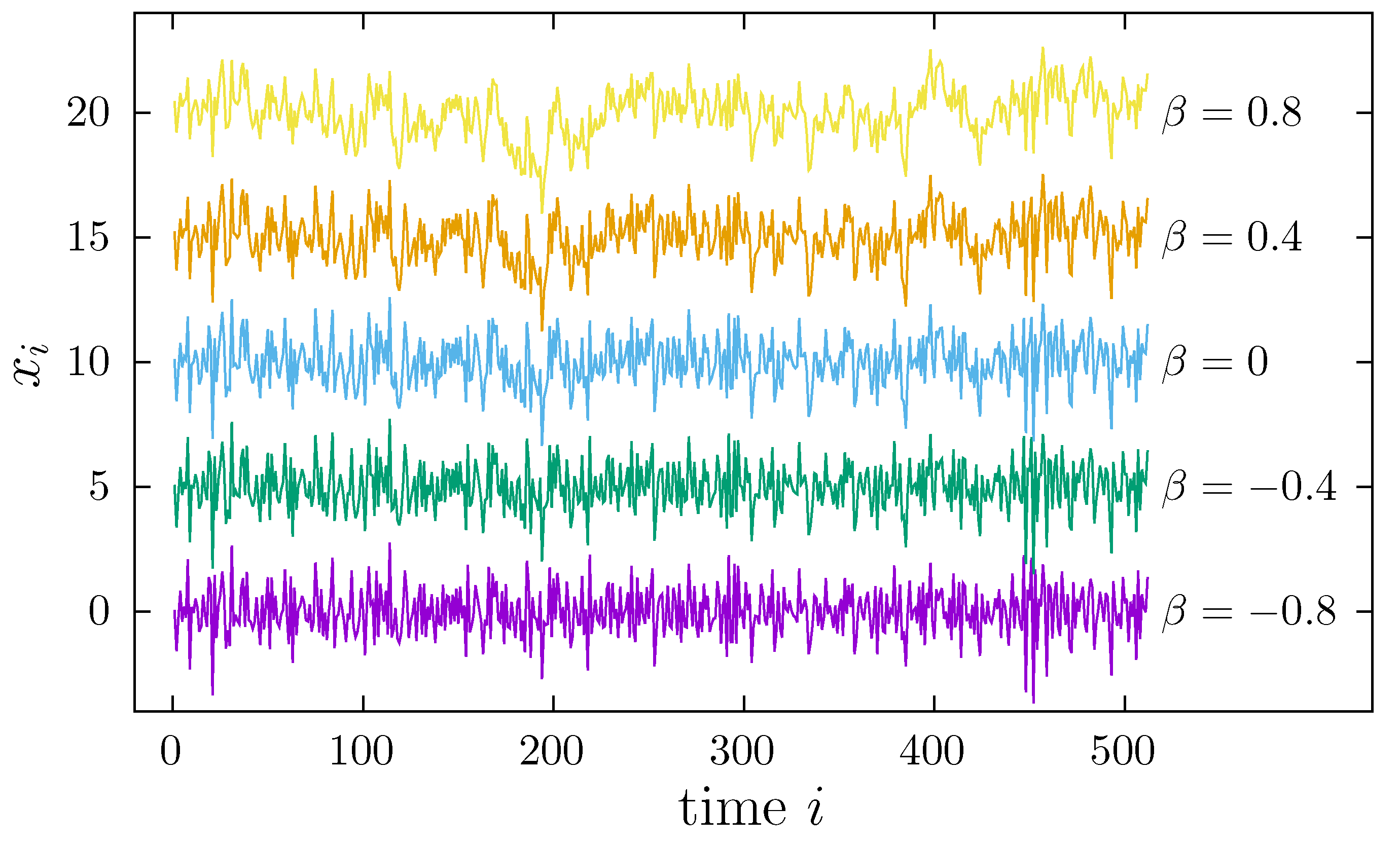
2. Fourier Filtering Method and $\mathbf{1}/{\mathit{f}}^{\mathit{\beta }}$ Noises

More precisely, the connection between the power-law behaviors of $S\left(f\right)$ and $C\left(k\right)$ described above motivated the use of algorithms utilizing simpler power spectra than (3) to synthetically generate power-law correlated times series. In particular, the most widely used is the Fourier filtering method (FFM) [17,18], which considers a power spectrum of the following type:

$$S\left(f\right)\sim \frac{1}{f^{\beta }},$$

(6)

therefore extending the behavior of (3) near the $f=0$ region to the entire range of frequencies. FFM works as follows: (a) Create a white noise $\left\{y_i\right\}$ $(i=1,\dots ,N)$ in the time domain and perform a Fourier transform to obtain $\left\{Y_f\right\}$. In this way, the corresponding discrete (positive) frequencies are given by the following.

$$f_i={\displaystyle \frac{i-1}{N}}.i=1,\dots ,N/2.$$

(7)

Multiply $\left\{Y_f\right\}$ by the filter $f^{-\beta /2}$ to obtain $\left\{X_f\right\}$. Fourier-transform $\left\{X_f\right\}$ back into time domain to obtain the final time series $\left\{x_i\right\}$ with N data points. By construction, time series $\left\{x_i\right\}$ presents a power spectrum as in Equation (6) such that the corresponding autocorrelation function behaves asymptotically as a power-law of type $C\left(k\right)\sim k^{1-\beta }$. For obvious reasons, the outputs $\left\{x_i\right\}$ of FFM are commonly known as $1/f^{\beta }$ noises or simply as $1/f$ noises, and in some contexts, they are also termed as colored noises. In Figure 1, we show several $1/f^{\beta }$ noises with $N=512$ data points obtained by using FFM with different input $\beta$ values.

Figure 1. Correlated time series with a power spectrum of the form $S\left(f\right)\sim 1/f^{\beta }$ obtained with the Fourier Filtering Method for several $\beta$ values. In all cases, the time series length is $N=512$. All series have 0 mean and unit standard deviation, but we have shifted them vertically to avoid overlapping.

The $1/f^{\beta }$ noises generated with FFM have become standard models for power-law correlated time series and are utilized for a great variety of purposes, such as benchmarks for techniques aimed at quantifying correlations [19,20,21,22,23], modeling correlated DNA sequences [24], studying return intervals and extreme events in correlated processes [25,26], or characterizing the localization properties of correlated–disordered chains [27,28,29]. In addition, we remark that the filtering process in FFM does not alter the Fourier phases, which are essentially random since they come from the Fourier transform of the original white noise. These random Fourier phases ensure that the final $1/f^{\beta }$ noise $\left\{x_i\right\}$ only possesses linear correlations such that $1/f^{\beta }$ noises are also used as prototypical power-law-correlated linear noises [30].

We note that, in the case of fGn, the duality $C\left(k\right)$-$S\left(f\right)$ is provided in Equations (1)–(3). However, despite the wide range of applications of $1/f^{\beta }$ noises and the simplicity of the corresponding power spectrum, to our knowledge, an explicit expression for the autocorrelation function of such noises is not known. This is the main aim of this paper. To this end, in Section 3, we present an analytical derivation of $C\left(k\right)$ for $1/f^{\beta }$ noises, including the exact result in terms of the Lommel functions and also an asymptotic expansion to illustrate the power-law behavior of $C\left(k\right)$ for these types of noises. We show the validity of our analytical results by comparing them with the numerical autocorrelation functions obtained for $1/f^{\beta }$ noises synthetically generated with FFM. Finally, in Section 4, we present two applications of our result. First, we compare the autocorrelation functions of fGn and $1/f^{\beta }$ noises and show some differences between them, especially in anticorrelated cases. Second, we obtain an exact expression for the Fluctuation Analysis algorithm [10,31], typically used to analyze correlated time series, when applied to $1/f^{\beta }$ noises.

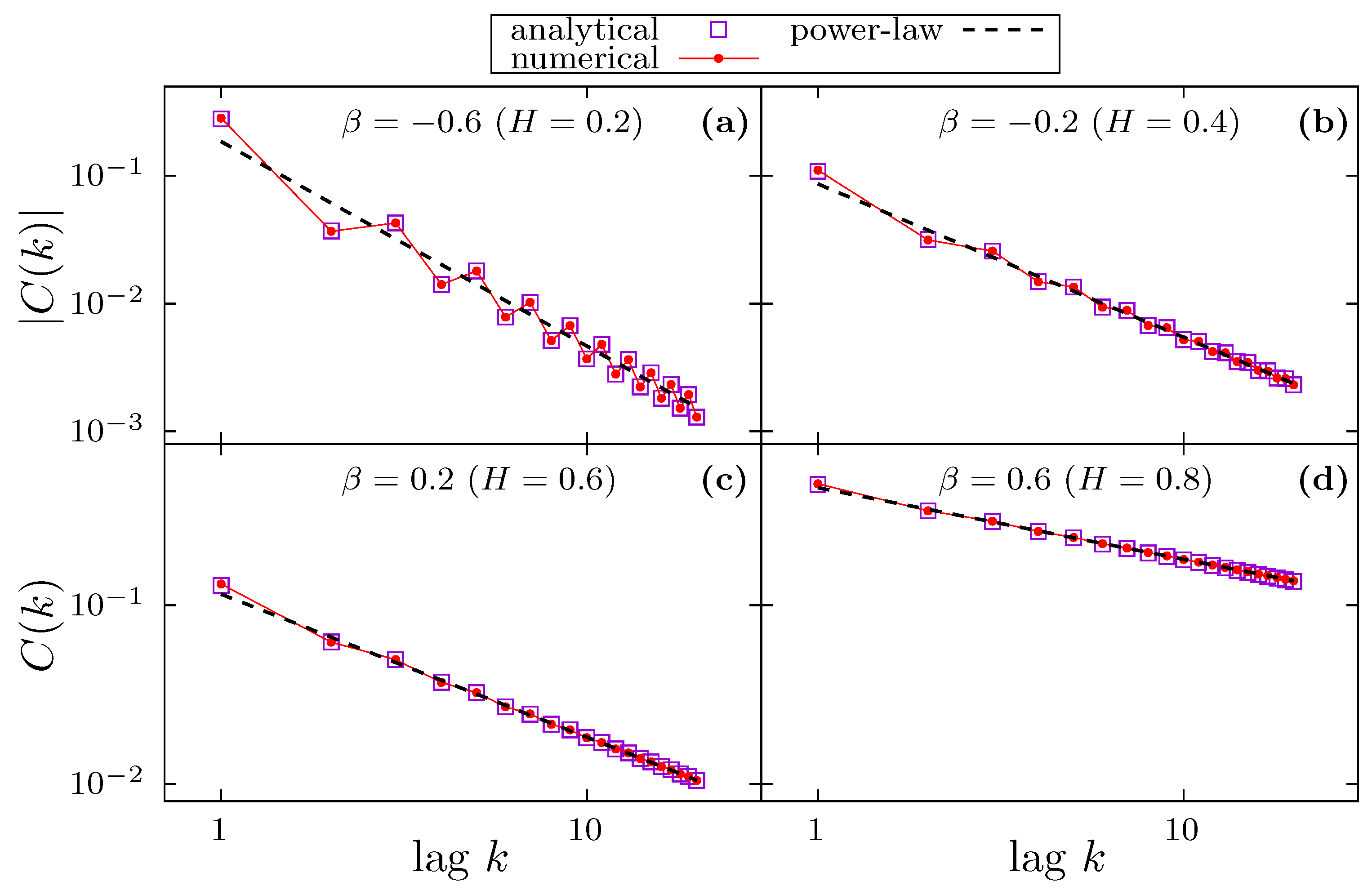
3. Autocorrelation Function of $\mathbf{1}/{\mathit{f}}^{\mathit{\beta }}$ Noises

Let us consider a time series of length N, $\{x_1,x_2,\dots ,x_N\}$, generated using the Fourier Filtering Method described in the previous section; therefore, the power spectrum $S\left(f\right)$ given by the following is obtained:

$$S\left(f\right)\sim \frac{1}{f^{\beta }}$$

with $\beta \in (-1,1)$ to ensure stationarity. Frequency f can have only discrete values given in Equation (7). According to the Wiener–Khinchin theorem, the autocovariance of an FFM time series can be obtained as the inverse discrete Fourier transform of $S\left(f\right)$. Therefore, autocorrelation $C\left(k\right)$ can be written as follows:

$$C\left(k\right)=\frac{{\sum }_{i=1}^{N/2}{f}_i^{-\beta }cos\left(2\pi k{f}_i\right)}{{\sum }_{i=1}^{N/2}{f}_i^{-\beta }},$$

where, again, the frequencies $f_i$ are given in (7), and we have used the parity of the power spectrum. Unfortunately, the expression for $C\left(k\right)$ does not have an analytical solution. However, if we consider the limit $N\to \infty$ of a very large time series, i.e., a $1/f^{\beta }$ process, we can exchange the sums by integrals and write the following:

$$C\left(k\right)=\frac{{\int }_0^{1/2}{f}^{-\beta }cos\left(2\pi kf\right)df}{{\int }_0^{1/2}{f}^{-\beta }df}.$$

(8)

In this case, the previous expression for $C\left(k\right)$ can be analytically evaluated. The integral in the denominator has the following value:

$${\int }_0^{1/2}{f}^{-\beta }df=\frac{2^{\beta -1}}{1-\beta }.$$

Concerning the integral in the numerator of (8), it can be written either in terms of the Lommel function or in terms of the generalized hypergeometric function (see Appendix A). We use the former option so that we can write the following:

$${\int }_0^{1/2}{f}^{-\beta }cos\left(2\pi kf\right)df=\frac{2^{\beta -1}}{1-\beta }\left(\frac{{(-1)}^{k-1}{s}_{\frac{3}{2}-\beta ,\frac{1}{2}}\left(k\pi \right)}{{\left(k\pi \right)}^{\frac{1}{2}-\beta }}+{(-1)}^k\right),$$

(9)

with $s_{\mu ,\nu }\left(z\right)$ being the first Lommel function [32] for which its main properties are briefly reviewed in Appendix A. By introducing the last two integrals in (8), we finally obtain the following:

$$C\left(k\right)={(-1)}^k+\frac{{(-1)}^{k-1}{s}_{\frac{3}{2}-\beta ,\frac{1}{2}}\left(k\pi \right)}{{\left(k\pi \right)}^{\frac{1}{2}-\beta }}.$$

(10)

This expression for $C\left(k\right)$ is exact, although it is not very illustrative due to the presence of $s_{\mu ,\nu }\left(z\right)$. Our aim here is to obtain a simpler expression for $C\left(k\right)$ characterizing its power-law behavior. To this end, we can calculate an asymptotic expansion of (10) in terms of lag k and consider in the expansion more than one term to account for small k values. We first note that, according to [33], we may write the following:

$$\begin{array}{ccc}\hfill s_{\mu ,\nu }\left(z\right)& =& S_{\mu ,\nu }\left(z\right)-2^{\mu -1}\Gamma \left(\frac{\mu +\nu +1}{2}\right)\Gamma \left(\frac{\mu -\nu +1}{2}\right)\hfill \\ & \times & \left[sin\left(\frac{\pi }{2}(\mu -\nu )\right)J_{\nu }\left(z\right)-cos\left(\frac{\pi }{2}(\mu -\nu )\right)Y_{\nu }\left(z\right)\right],\hfill \end{array}$$

(11)

where $J_{\nu }\left(z\right)$ and $Y_{\nu }\left(z\right)$ are the Bessel functions, and $S_{\mu ,\nu }\left(z\right)$ is the second Lommel function [32]. $S_{\mu ,\nu }\left(z\right)$ admits an asymptotic expansion as $z\to \infty$ given by the following:

$$S_{\mu ,\nu }\left(z\right)\sim z^{\mu -1}\sum _{j=0}^{\infty }{(-1)}^j{a}_j(-\mu ,\nu )z^{-2j},$$

(12)

where the coefficients $a_j(\mu ,\nu )$ are defined as:

$$a_j(\mu ,\nu )=\prod _{m=1}^j({(\mu +2m-1)}^2-{\nu }^2),j=0,1,2,\dots .$$

(13)

Using these two last equations, the first terms of the asymptotic expansion of $S_{\mu ,\nu }\left(z\right)$ are as follows:

$$S_{\mu ,\nu }\left(z\right)=z^{\mu -1}-\frac{{(1-\mu )}^2-{\nu }^2}{z^{3-\mu }}+\mathcal{O}\left(\frac{1}{z^{5-\mu }}\right).$$

By introducing this expansion in (11) and noting that $\mu =3/2-\beta$ and $\nu =1/2$, we obtain the following:

$$\begin{array}{ccc}\hfill s_{\frac{3}{2}-\beta ,\frac{1}{2}}\left(z\right)& =& \frac{1}{z^{\beta -\frac{1}{2}}}-\frac{\beta (\beta -1)}{z^{\beta +\frac{3}{2}}}+\mathcal{O}\left(\frac{1}{z^{\beta +\frac{7}{2}}}\right)-2^{1-\beta }\frac{\Gamma \left(\frac{3-\beta }{2}\right)\Gamma \left(\frac{2-\beta }{2}\right)}{\sqrt{\pi z}}\times \hfill \\ & \times & \left[sin\left(\frac{\pi }{2}(1-\beta )\right)sinz+cos\left(\frac{\pi }{2}(1-\beta )\right)cosz\right],\hfill \end{array}$$

(14)

where we have used that for $\nu =1/2$ the Bessel functions are given by the following expressions:

$$J_{\frac{1}{2}}\left(z\right)=\frac{\sqrt{2}sinz}{\sqrt{\pi z}},Y_{\frac{1}{2}}\left(z\right)=-\frac{\sqrt{2}cosz}{\sqrt{\pi z}}.$$

Equation (14) can be simplified notably: First, using the properties of the gamma function (Legendre duplication formula), we can write the product of gamma functions in (14) as:

$$\Gamma \left(\frac{3-\beta }{2}\right)\Gamma \left(\frac{2-\beta }{2}\right)=2^{\beta -1}\sqrt{\pi }\Gamma (2-\beta ).$$

Second, we can also simplify the term within brackets in Equation (14) as:

$$sin\left(\frac{\pi }{2}(1-\beta )\right)sinz+cos\left(\frac{\pi }{2}(1-\beta )\right)cosz=cos\left(z-\frac{\pi }{2}(1-\beta )\right)=sin\left(z+\frac{\beta \pi }{2}\right)$$

Using these two simplifications and noting that, according to (10), the argument of the Lommel function is $z=k\pi$, we obtain the following from Equation (14):

$$s_{\frac{3}{2}-\beta ,\frac{1}{2}}\left(k\pi \right)={(-1)}^{k+1}\frac{\Gamma (2-\beta )sin\left(\frac{\beta \pi }{2}\right)}{\sqrt{k\pi }}+\frac{1}{{\left(k\pi \right)}^{\beta -\frac{1}{2}}}-\frac{\beta (\beta -1)}{{\left(k\pi \right)}^{\beta +\frac{3}{2}}}+\mathcal{O}\left(\frac{1}{{\left(k\pi \right)}^{\beta +\frac{7}{2}}}\right),$$

where we have used the equality $sin\left(k\pi +\beta \pi /2\right)={(-1)}^{k}sin\left(\beta \pi /2\right)$. By inserting this result for $s_{\frac{3}{2}-\beta ,\frac{1}{2}}\left(k\pi \right)$ into (10), we finally obtain the following expression for $C\left(k\right)$:

$$C\left(k\right)={\displaystyle \frac{\Gamma (2-\beta )sin\left(\frac{\pi }{2}\beta \right)}{{\left(k\pi \right)}^{1-\beta }}}+{(-1)}^k{\displaystyle \frac{\beta (\beta -1)}{{\left(k\pi \right)}^2}}+\mathcal{O}\left(\frac{1}{k^4}\right).$$

(15)

This equation is the main result of this paper. The right-hand side of (15) contains two terms, where the first one corresponds to the asymptotic power-law behavior $C\left(k\right)\sim k^{\beta -1}$. The second term describes a correction with respect to the power-law for small lag k values. Due to the presence of the ${(-1)}^k$ factor in this second term, the correction will have alternate sign for even and odd k values, so we expect, for small k, an oscillatory behavior of $C\left(k\right)$ around the asymptotic power-law with amplitude decreasing as $1/k^2$. We expect the oscillatory correction to be important for negative $\beta$ values (anticorrelated noises) since, in this case, the power-law values are small in absolute values, and factor $\beta (\beta -1)$ is large, especially for $\beta$ values close to $-1$ (strong anticorrelations). We remark that the oscillatory behavior of $C\left(k\right)$ is not a finite size effect, since Equation (8) has been obtained in the $N\to \infty$ limit, but an intrinsic property which is a consequence derived from the perfect power-law behavior of $S\left(f\right)$.

In order to illustrate the validity of the analytical result (15), we show, in Figure 2, a comparison of the autocorrelation function of time series generated using the FFM algorithm for different $\beta$ values and the corresponding $C\left(k\right)$ function obtained using (15). For each $\beta$ value, we generate a single time series with $N=2^{22}$ data points. We observed how the numerically obtained $C\left(k\right)$ function matches perfectly with the result in Equation (15). In addition, according to our prediction, we observe an oscillatory behavior of $C\left(k\right)$ around the corresponding asymptotic power-law (first term in Equation (15)), which is shown with dashed lines in Figure 1. These oscillations are more pronounced for negative $\beta$ values, which is in agreement with the second term in Equation (15), and reduce considerably as $\beta$ increases and becomes positive.

Figure 2. Autocorrelation function of $1/f^{\beta }$ noises with different $\beta$ values: $-0.6$ (a), $-0.2$ (b), $0.2$ (c), and $0.6$ (d). For $\beta =-0.6$ and $-0.2$ (negative $C\left(k\right)$), we plot $\left|C\right(k\left)\right|$ to use logarithmic scales in both axes. In all panels, small connected circles correspond to the numerical $C\left(k\right)$ obtained for synthetic FFM time series with $N=2^{22}$, squares correspond to the analytical solution in Equation (15), and the dashed lines correspond to the asymptotic power-law behavior (first term of Equation (15)).

4. Applications

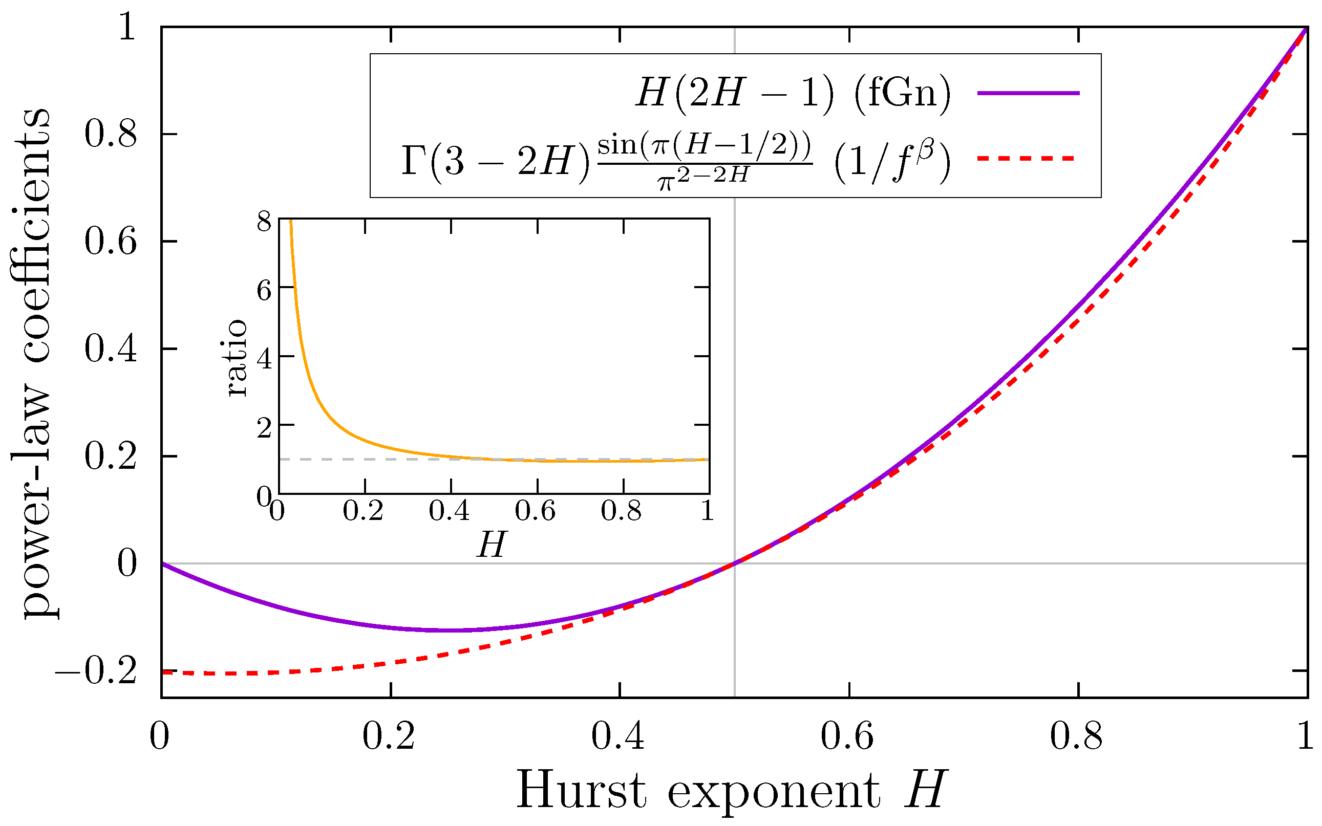
4.1. Comparing fGn and $1/f^{\beta }$ Noises

Formula (15) can be also written in terms of the Hurst exponent H. As $\beta =2H-1$, from (15), we can write $C\left(k\right)$ as follows:

$$C\left(k\right)={\displaystyle \frac{\Gamma (3-2H)sin\left(\pi \left(H-\frac{1}{2}\right)\right)}{{\left(k\pi \right)}^{2-2H}}}+{(-1)}^k{\displaystyle \frac{(2H-1)(2H-2)}{{\left(k\pi \right)}^2}}+\mathcal{O}\left(\frac{1}{k^4}\right).$$

(16)

This last expression allows a direct comparison with the autocorrelation function of fractional Gaussian noise with the same Hurst exponent H and, therefore, with a similar asymptotic power-law behavior. In this regime, we compare, in Figure 3, the coefficients of the $1/k^{2-2H}$ term in Equations (2) and (16), and we observe the following:

$${\displaystyle \frac{\Gamma (3-2H)sin\left(\pi \left(H-\frac{1}{2}\right)\right)}{{\pi }^{2-2H}}}\le H(2H-1)$$

(17)

for $H\in (0,1)$. The equality only holds for $H=1/2$ (white noise), where both expressions are null. Therefore, in general, the autocorrelations of fGn-type time series are larger than those of $1/f^{\beta }$ noises generated with the same Hurst exponent H. Note that, for $H>1/2$, corresponding to long-range positively correlated time series, the difference between the two power-law coefficients is very small such that both kind of noises, fGn and $1/f^{\beta }$, exhibit autocorrelation functions with almost identical asymptotic behavior not only with the same power-law exponent but also with the same correlation strength.

Figure 3. Coefficients of the asymptotic power-law behavior of the autocorrelation functions of fGn (solid line) and $1/f^{\beta }$ noises (dashed line) as a function of the Hurst exponent H. Inset: The ratio of the power-law coefficients of $1/f^{\beta }$ noises over fGn also as a function of H. The horizontal dashed line corresponds to a ratio equal to unity.

However, for the case $H<1/2$, the correlations are negative; although those for fGn are larger than for $1/f^{\beta }$ noises, they are smaller in absolute values (closer to 0). This difference is particularly relevant for strong anticorrelated power-law behavior, i.e., for H values close to 0, where (in absolute value) the fGn coefficient (solid line in Figure 3) can be much smaller than the $1/f^{\beta }$ noise coefficient (dashed line in Figure 3). This property can be better appreciated in the inset of Figure 3, where we plot the ratio between the corresponding coefficients of $1/f^{\beta }$ noises and fGn, and we show how the ratio between them diverges as $H\to 0$. This property may be a drawback when using fGn to model power-law anticorrelated time series, i.e., for $H<1/2$. Note that, for a synthetic time series with N data points, the noise level for the autocorrelation values is around $\pm 2/\sqrt{N}$ [34], so values within this range are not significant. Since both fGn and $1/f^{\beta }$ autocorrelation functions are decaying (in absolute value) power-laws with the same exponent, the smaller coefficient for the fGn case produces that the corresponding $C\left(k\right)$ reaches the noise level sooner (for smaller k values) than for $1/f^{\beta }$ noises. In this sense, the $C\left(k\right)$-significant power-law behavior for anticorrelated $1/f^{\beta }$ noises can be observed for a longer range of lag k values than for fGn generated with the same $H<1/2$ value. For this reason, $1/f^{\beta }$ noises should be the model of choice when studying power-law anticorrelated time series.

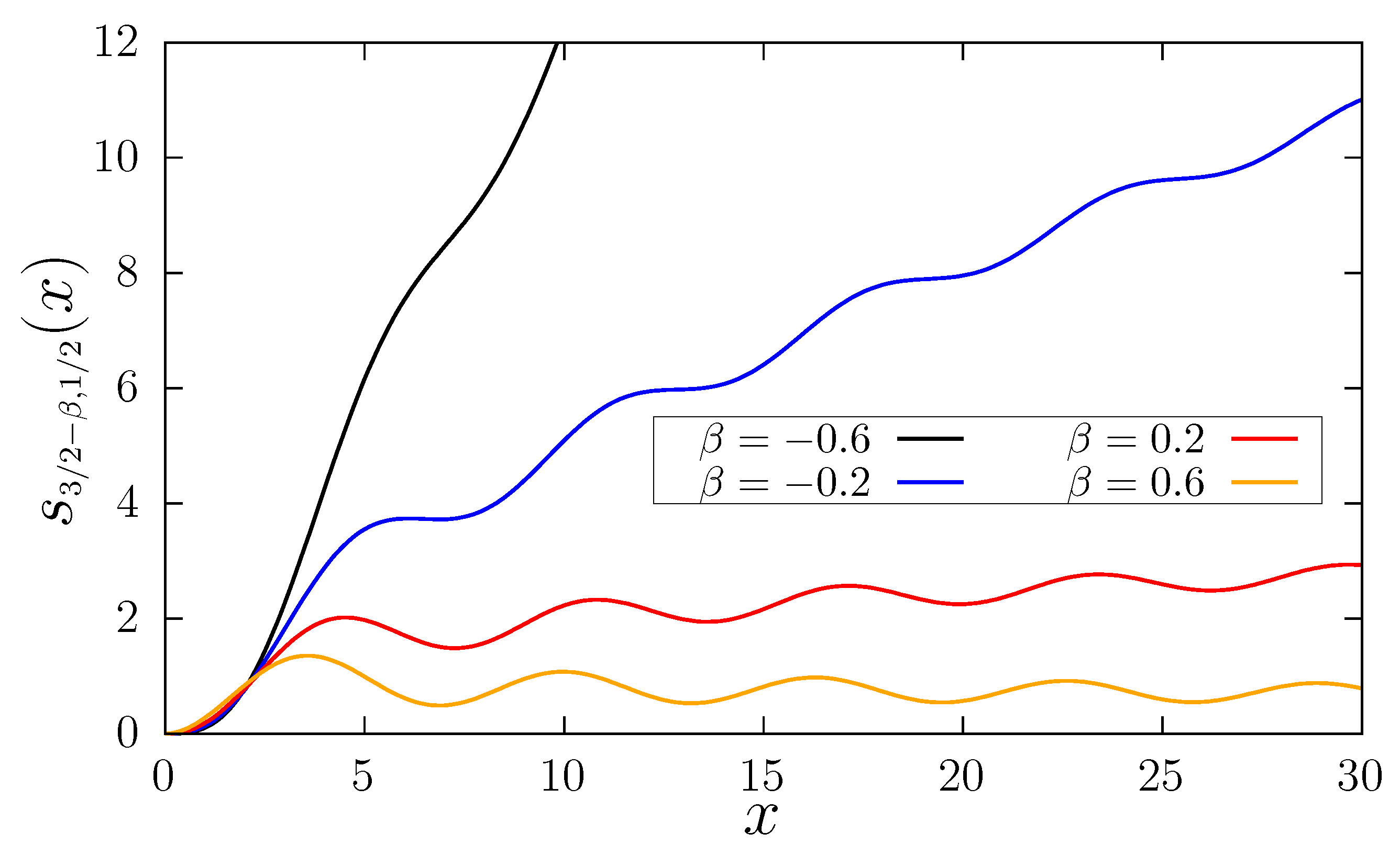
4.2. Fluctuation Analysis of $\mathit{1}/f^{\beta }$ Noises

Fluctuation Analysis (FA) [10,31] is a technique commonly applied in the analysis of times series aimed at calculating the scaling properties of the fluctuations of a given signal. The underlying idea of FA is the interpretation of the analyzed time series $\left\{x_i\right\}$ as the steps of a walk in a diffusion process, and then the “accumulated walk” $X_j$ of the signal is considered as follows:

$$X_j=\sum _{i=1}^j{x}_i.$$

The FA algorithm computes the averaged diffused distance after ℓ steps as the Mean Square Distance $F(\ell )$ obtained as follows:

$$F(\ell )=\sqrt{⟨{(X_{i+\ell }-X_i)}^2⟩},$$

(18)

where $⟨\dots ⟩$ means the average over the entire time series. The analyzed signal presents scaling when $F(\ell )\sim {\ell }^H$, with H being the Hurst exponent. Usually, FA is applied numerically to the target time series, and the scaling exponent H is obtained as the slope of a linear fitting of $log\left(F\right(\ell \left)\right)$ vs. $log(\ell )$. FA is typically tested using FFM-generated $1/f^{\beta }$ noises, and the results allow numerically verifying the relation between exponents $\beta =2H-1$.

We recall that a connection between the $F(\ell )$ function of a given time series and the corresponding autocorrelation function $C\left(k\right)$ is known [22,35]:

$$F^2(\ell )={\sigma }^2\left(\ell +2\sum _{k=1}^{\ell -1}(\ell -k)C\left(k\right)\right),$$

(19)

with ${\sigma }^2$ denoting the variance of the time series. This result can be used to obtain an exact expression for FA function $F(\ell )$ of $1/f^{\beta }$ noises, since we already know the corresponding expressions of $C\left(k\right)$, both in the exact (10) and the asymptotic (15) forms. Since the sum in Equation (19) involves small values of lag k, it is convenient to use the exact expression for $C\left(k\right)$ given in Equation (10); after introducing it in (19) and performing simplification, we finally obtain the following:

$$\begin{array}{ccc}\hfill F^2(\ell ))& =& {\sigma }^2\left[\frac{1-{(-1)}^{\ell }}{2}+2\sum _{k=1}^{\ell -1}\left((\ell -k)\frac{{(-1)}^{k-1}{s}_{3/2-\beta ,1/2}\left(k\pi \right)}{{\left(k\pi \right)}^{\frac{1}{2}-\beta }}\right)\right]\hfill \\ & =& {\sigma }^2\left[\frac{1-{(-1)}^{\ell }}{2}+2\sum _{k=1}^{\ell -1}\left((\ell -k)\frac{{(-1)}^{k-1}{s}_{5/2-2H,1/2}\left(k\pi \right)}{{\left(k\pi \right)}^{\frac{3}{2}-2H}}\right)\right].\hfill \end{array}$$

(20)

As we show in Figure 4, this result agrees perfectly with the $F(\ell )$ function obtained numerically by applying the FA algorithm in Equation (18) to $1/f^{\beta }$ noises generated with the FFM algorithm.

Figure 4. FA functions $F(\ell )$ obtained for $1/f^{\beta }$ noises using different input Hurst exponents $H=2\beta -1$. The solid lines are obtained by plotting the analytical result (20), while the symbols correspond to the numerical results obtained by applying (18) to $1/f^{\beta }$ noises with $N=2^{20}$ generated using FFM.

Another technique widely used to quantify the scaling properties of a given time series is Detrended Fluctuation Analysis (DFA) [36], a generalization of FA also valid for non-stationary signals. Similarly to FA, DFA provides a fluctuation function $F(\ell )$, and when scaling is present, it holds that $F(\ell )\sim {\ell }^H$. For DFA, an expression similar to (19) (although more complicated) relating $F(\ell )$ and $C\left(k\right)$ has been obtained in [37]. Therefore, using this expression, the analytical behavior of DFA for $1/f^{\beta }$ noises can be obtained, which we do not present here for brevity. This result for DFA, together with the result for FA in Equation (20), can be useful to understand the deviation of $F(\ell )$ from the expected power-law behavior observed numerically at small values of ℓ when analyzing $1/f^{\beta }$ noises with FA and DFA [23].

5. Conclusions

We have obtained an analytical derivation of the autocorrelation function $C\left(k\right)$ of $1/f^{\beta }$ noises which, to our knowledge, was not known explicitly, despite the wide range of applications of such noises. We provide the exact result in terms of the Lommel functions and an asymptotic expansion including the power-law behavior and a oscillatory correction for small values of lag k. These results are in agreement with the autocorrelation functions obtained from synthetically generated $1/f^{\beta }$ times series using the Fourier filtering method.

In addition to better characterizing the correlations of $1/f^{\beta }$ noises, our results allow comparisons to other noises with, in principle, similar power-law correlations, specifically to fractional Gaussian noise. Both noises depend on the same parameter, the Hurst exponent H, which controls the exponent of the power-law-behaved autocorrelation functions; therefore, both noises should behave similarly provided that they are generated with the same H value. Indeed, this is the case for $H>1/2$ (positive correlations), where the autocorrelation functions are similar power laws not only in the power-law exponent (which is identical) but also in the value of the multiplicative constant of such power laws. However, for negative correlations ($H<1/2$), even though the power-law exponents are identical, the multiplicative constant of $1/f^{\beta }$ noises is larger in absolute values than the one of fGn, and the ratio between them diverges as $H\to 0$. This implies that (in absolute value) the correlation values are larger for $1/f^{\beta }$ noises than for fGn for the same value of lag k. This result suggests that when modeling power-law anticorrelated time series of finite length N, the model of choice should be $1/f^{\beta }$ noises (specially for small H values), since in this case, the observable and significant power-law behavior extends over a larger range of k values than for fractional Gaussian noise.

The knowledge of an explicit expression of $C\left(k\right)$ for $1/f^{\beta }$ noises allows analytically obtaining the behavior of other indirect techniques aimed at quantifying correlations, such as FA and DFA, when applied to these types of noise. Finally, as another future possible application, $C\left(k\right)$ could be considered to compare two cellular automata systems where the number of living cells follows a power-law behavior [11].

References

- Hurst, H.E. Long-term storage capacity of reservoirs. Trans. Am. Soc. Civ. Eng. 1951, 116, 770–779. [Google Scholar] [CrossRef]
- Peters, E.E. Fractal Market Analysis: Applying Chaos Theory to Investment and Economics; John Wiley & Sons: Hoboken, NJ, USA, 1994. [Google Scholar]
- Peng, C.K.; Mietus, J.; Hausdorff, J.M.; Havlin, S.; Stanley, H.E.; Goldberger, A.L. Long-range anticorrelations and non-Gaussian behavior of the heartbeat. Phys. Rev. Lett. 1993, 70, 1343–1346. [Google Scholar] [CrossRef] [PubMed]
- Ivanov, P.C. Long-range dependence in heartbeat dynamics. In Processes with Long Range Correlations: Theory and Applications (Lecture Notes in Physics Vol. 621); Rangajaran, G., Ding, M., Eds.; Springer: Berlin/Heidelberg, Germany, 2003; pp. 339–372. [Google Scholar]
- Ivanov, P.C. From 1/f noise to multifractal cascades in heartbeat dynamics. Chaos 2001, 11, 641–652. [Google Scholar] [CrossRef] [PubMed] [Green Version]
- Peng, C.K.; Mietus, J.E.; Liu, Y.; Lee, C.; Hausdorff, J.M.; Stanley, H.E.; Goldberger, A.L.; Lipsitz, L.A. Quantifying fractal dynamics of human respiration: Age and gender effects. Ann. Biomed. Eng. 2002, 30, 683–692. [Google Scholar] [CrossRef]
- Likenkaer-Hansen, K.; Nikouline, V.V.; Palva, J.M.; Ilmoniemi, R.J. Long-range temporal correlations and scaling behavior in human brain oscillations. J. Neurosci. 2001, 21, 1370–1377. [Google Scholar] [CrossRef] [Green Version]
- Duarte, M.; Zatsiorski, V.M. On the fractal properties of natural human standing. Neurosci. Lett. 2000, 283, 173–176. [Google Scholar] [CrossRef]
- Blázquez, M.T.; Anguiano, M.; de Saavedra, F.; Lallena, A.M.; Carpena, P. Study of the human postural control system during quiet standing using detrended fluctuation analysis. Physica A 2009, 388, 1857–1866. [Google Scholar] [CrossRef]
- Peng, C.K.; Buldyrev, S.V.; Goldberger, A.L.; Havlin, S.; Sciortino, F.; Simons, M.; Stanley, H.E. Long-range correlations in nucleotide sequences. Nature 1992, 356, 168–170. [Google Scholar] [CrossRef]
- Contreras-Reyes, J.E. Lerch distribution based on maximum nonsymmetric entropy principle: Application to Conway’s Game of Life cellular automaton. Chaos Solitons Fractals 2021, 151, 111272. [Google Scholar] [CrossRef]
- Bartos, I.; Jánosi, I.M. Nonlinear correlations of daily temperature records over land. Nonlin. Process. Geophys. 2006, 13, 571–576. [Google Scholar] [CrossRef] [Green Version]
- Varotsos, A.; Sarlis, N.V.; Skordas, E.S. Long-range correlations in the electric signals that precede rupture. Phys. Rev. E 2002, 66, 011902. [Google Scholar] [CrossRef] [PubMed] [Green Version]
- Mandelbrot, B.B.; Van Ness, J.W. Fractional Brownian motions, fractional noises ans applications. SIAM Rev. 1968, 10, 422–437. [Google Scholar] [CrossRef]
- Davies, R.B.; Harte, D.S. Test for Hurst Effect. Biometrika 1987, 74, 95–101. [Google Scholar] [CrossRef]
- Dieker, A.B.; Mandjes, M. On spectral simulation of fractional Brownian motion. Probab. Eng. Inf. Sci. 2003, 17, 417–434. [Google Scholar] [CrossRef] [Green Version]
- Makse, H.A.; Havlin, S.; Schwartz, M.; Stanley, H.E. Method for generating long-range correlations for large systems. Phys. Rev. E 1996, 53, 5445–5449. [Google Scholar] [CrossRef] [PubMed] [Green Version]
- Rangarajan, G.; Ding, M. Integrated approach to the assessment of long range correlation in time series data. Phys. Rev. E 2000, 61, 4991. [Google Scholar] [CrossRef] [Green Version]
- Coronado, A.V.; Carpena, P. Size Effects on Correlation Measures. J. Biol. Phys. 2005, 31, 121–133. [Google Scholar] [CrossRef] [Green Version]
- Hu, K.; Ivanov, P.C.; Chen, Z.; Carpena, P.; Stanley, H.E. Effect of trends on detrended fluctuation analysis. Phys. Rev. E 2001, 64, 011114. [Google Scholar] [CrossRef] [Green Version]
- Chen, Z.; Hu, K.; Carpena, P.; Bernaola-Galván, P.; Stanley, H.E.; Ivanov, P.C. Effect of nonlinear filters on detrended fluctuation analysis. Phys. Rev. E 2005, 71, 011104. [Google Scholar] [CrossRef] [Green Version]
- Carpena, P.; Gómez-Extremera, M.; Carretero-Campos, C.; Bernaola-Galván, P.A.; Coronado, A.V. Spurious Results of Fluctuation Analysis Techniques in Magnitude and Sign Correlations. Entropy 2017, 19, 261. [Google Scholar] [CrossRef]
- Carpena, P.; Gómez-Extremera, M.; Bernaola-Galván, P.A. On the Validity of Detrended Fluctuation Analysis at Short Scales. Entropy 2022, 24, 61. [Google Scholar] [CrossRef] [PubMed]
- Carpena, P.; Bernaola-Galván, P.; Coronado, A.V.; Hackenberg, M.; Oliver, J.L. Identifying characteristic scales in the human genome. Phys. Rev. E 2007, 75, 032903. [Google Scholar] [CrossRef] [PubMed] [Green Version]
- Carretero-Campos, C.; Bernaola-Galván, P.A.; Ivanov, P.C.; Carpena, P. Phase transitions in the first-passage time of scale-invariant correlated processes. Phys. Rev. E 2012, 85, 011139. [Google Scholar] [CrossRef] [PubMed] [Green Version]
- Kalraa, D.S.; Santhanamb, M.S. Inferring long memory using extreme events. Chaos 2021, 31, 113131. [Google Scholar] [CrossRef]
- de Moura, F.A.B.F.; Lyra, M.L. Delocalization in the 1D Anderson model with long-range correlated disorder. Phys. Rev. Lett. 1998, 81, 3735–3738. [Google Scholar] [CrossRef]
- Nguyen, B.P.; Thoa, T.K.; Kim, K. Numerical study of the transverse localization of waves in one-dimensional lattices with randomly distributed gain and loss: Effect of disorder correlations. Waves Random Complex Media 2022, 32, 390–405. [Google Scholar] [CrossRef]
- Pires, J.P.S.; Khan, N.A.; Lopes, J.M.V.P.; dos Santos, J.M.B.L. Global delocalization transition in the de Moura-Lyra model. Phys. Rev. B 2019, 99, 205148. [Google Scholar] [CrossRef] [Green Version]
- Carpena, P.; Bernaola-Galván, P.; Gómez-Extremera, M.; Coronado, A.V. Transforming Gaussian correlations. Applications to generating long-range power-law correlated time series with arbitrary distribution. Chaos 2020, 30, 083140. [Google Scholar] [CrossRef]
- Bryce, R.M.; Sprague, K.B. Revisiting detrended fluctuation analysis. Sci. Rep. 2012, 2, 315. [Google Scholar] [CrossRef] [Green Version]
- Abramowitz, M.; Stegun, I. Handbook of Mathematical Functions with Formulas, Graphs, and Mathematical Tables; Ninth Printing; Dover Publications: New York, NY, USA, 1964. [Google Scholar]
- Olver, F.W.J.; Lozier, D.W.; Boisvert, R.F.; Clark, C.W. NIST Handbook of Mathematical Functions; Cambridge University Press: New York, NY, USA, 2010. [Google Scholar]
- Beran, J. Statistics for Long-Memory Processes; Chapman and Hall/CRC: New York, NY, USA, 1994. [Google Scholar]
- Karlin, S.; Brendel, V. Patchiness and correlations in DNA sequences. Science 1993, 259, 677–680. [Google Scholar] [CrossRef]
- Peng, C.K.; Buldyrev, S.V.; Havlin, S.; Simons, M.; Stanley, H.E.; Goldberger, A.L. Mosaic organization of DNA nucleotides. Phys. Rev. E 1994, 49, 1685–1689. [Google Scholar] [CrossRef] [PubMed] [Green Version]
- Höll, M.; Kantz, H. The relationship between the detrended fluctuation analysis and the autocorrelation function of a signal. Eur. Phys. J. B 2015, 88, 327. [Google Scholar] [CrossRef]
- Gradshteyn, I.S.; Ryzhik, I.M. Tables of Integrals, Series and Products, 7th ed.; Jeffrey, A., Zwillinger, D., Eds.; Academic Press: Cambridge, MA, USA, 2007. [Google Scholar]
Publisher’s Note: MDPI stays neutral with regard to jurisdictional claims in published maps and institutional affiliations. |
© 2022 by the authors. Licensee MDPI, Basel, Switzerland. This article is an open access article distributed under the terms and conditions of the Creative Commons Attribution (CC BY) license (https://creativecommons.org/licenses/by/4.0/).