Article

Elite Directed Particle Swarm Optimization with Historical Information for High-Dimensional Problems

School of Artificial Intelligence, Nanjing University of Information Science and Technology, Nanjing 210044, China
*
Author to whom correspondence should be addressed.
Mathematics 2022, 10(9), 1384; https://doi.org/10.3390/math10091384
Submission received: 11 March 2022 / Revised: 14 April 2022 / Accepted: 18 April 2022 / Published: 20 April 2022
(This article belongs to the Special Issue Recent Advances in Computational Intelligence and Its Applications)

Abstract

:
High-dimensional optimization problems are ubiquitous in every field nowadays, which seriously challenge the optimization ability of existing optimizers. To solve this kind of optimization problems effectively, this paper proposes an elite-directed particle swarm optimization (EDPSO) with historical information to explore and exploit the high-dimensional solution space efficiently. Specifically, in EDPSO, the swarm is first separated into two exclusive sets based on the Pareto principle (80-20 rule), namely the elite set containing the top best 20% of particles and the non-elite set consisting of the remaining 80% of particles. Then, the non-elite set is further separated into two layers with the same size from the best to the worst. As a result, the swarm is divided into three layers. Subsequently, particles in the third layer learn from those in the first two layers, while particles in the second layer learn from those in the first layer, on the condition that particles in the first layer remain unchanged. In this way, the learning effectiveness and the learning diversity of particles could be largely promoted. To further enhance the learning diversity of particles, we maintain an additional archive to store obsolete elites, and use the predominant elites in the archive along with particles in the first two layers to direct the update of particles in the third layer. With these two mechanisms, the proposed EDPSO is expected to compromise search intensification and diversification well at the swarm level and the particle level, to explore and exploit the solution space. Extensive experiments are conducted on the widely used CEC’2010 and CEC’2013 high-dimensional benchmark problem sets to validate the effectiveness of the proposed EDPSO. Compared with several state-of-the-art large-scale algorithms, EDPSO is demonstrated to achieve highly competitive or even much better performance in tackling high-dimensional problems.

1. Introduction

With the rapid development of big data and the Internet of Things (IoT), the dimensionality of optimization problems is becoming increasingly higher and higher [1,2], leading to the emergence of high-dimensional optimization problems [3,4,5]. Such a kind of optimization problem brings many undesirable challenges to existing optimizers. Specifically, with the dimensionality increasing, the solution space of optimization problems grows exponentially, resulting in the search effectiveness and the efficiency of existing optimizers degrading dramatically [6]. On the other hand, wide and flat local regions are also likely to increase rapidly as the dimensionality grows, especially for multimodal problems. This results in it being hard for existing optimizers to effectively escape from local areas, such that global optima cannot be located efficiently [7,8].
To address the above challenges, a lot of metaheuristic algorithms have been proposed by taking inspiration from nature and other disciplines. For example, imitating the laws of physics, physics-based optimization algorithms such as Henry gas solubility optimization (HGSO) [9], and artificial electric field algorithm (AEFA) [10], have been developed. Inspired by the social behaviors of animals, swarm intelligence optimization algorithms, such as particle swarm optimization (PSO) [11,12], ant colony optimization (ACO) [13,14,15], salp swarm algorithm (SSA) [16] and grey wolf optimization (GWO) [17], have been devised. Derived from competitive behaviors in sport playing, sport inspiration algorithms, such as the most valuable player algorithm (MVPA) [18] have been designed. Arisen from theories in mathematics, mathematics inspiration optimization, such as arithmetic optimization algorithm (AOA) [19] and sine cosine algorithm (SCA) [20], have been proposed. Inspired by the thoughts of species evolution, evolutionary algorithms, such as genetic algorithms (GA) [21] and differential evolution algorithms (DE) [22,23], have been developed. In addition, some other metaheuristic algorithms, such as adaptive hybrid approach (AHA) [24], Harris hawks optimization (HHO) [25], hunger games search (HGS) [26] and golden jackal optimization (GJO) [27], have also been designed to solve optimization problems.
Among the above different kinds of metaheuristic algorithms, PSO has been researched the most in dealing with large-scale optimization [28,29,30,31,32]. In a broad sense, existing PSO research for high-dimensional optimization problems can be categorized into two main directions [33]: cooperative co-evolutionary PSOs (CCPSOs) [34,35,36] and holistic large-scale PSOs [37,38,39,40,41].
CCPSOs [42,43] first adopt the divide-and-conquer technique to divide a high-dimensional problem into a number of low-dimensional sub-problems, and then utilize traditional PSOs for low-dimensional problems to separately solve the decomposed sub-problems. Since Potter [44] proposed the cooperative co-evolutionary (CC) framework, researchers have employed this framework into different evolutionary algorithms and developed many cooperative co-evolutionary algorithms (CCEAs) [43,45], among which CCPSOs [35,46] have been developed by introducing PSOs into the CC framework.
However, the optimization performance of CCEAs including CCPSOs heavily relies on the decomposition accuracy in dividing the high-dimensional problem into sub-problems, since the optimization of interacting variables usually interferes with each other [43]. Ideally, a good decomposition strategy should place interacting variables into the same sub-problem, so that they can be optimized together. Nevertheless, without prior knowledge on the correlations between variables, it is hard to accurately decompose a high-dimensional problem into sub-problems. To solve this issue, researchers have been devoted to designing effective decomposition strategies to divide a high-dimensional problem into sub-problems as accurately as possible by detecting the correlations between variables [47]. As a consequence, a lot of remarkable decomposition strategies [48,49,50,51,52] have been devised and assisted CCEAs, including CCPSOs, to achieve very promising performance in tackling large-scale optimization.
Different from CCPSOs, holistic large-scale PSOs [33,53] still consider optimizing all variables together such as traditional PSOs. The key role in designing effective holistic large-scale PSOs lies in devising effective learning strategies for PSO to improve the search diversity, largely so that particles in the swarm could search the solution space in different directions and locate the promising areas fast. To achieve this goal, researchers have abandoned historical information, such as the personal best positions pbests, the global best position gbest, or the neighbor best position nbest, and attempted to employ predominate particles in the current swarm to guide the learning of poor particles. Along this line, many novel effective learning strategies [29,31,32,54,55] have been proposed, such as the competitive learning strategy [29], the level-based learning strategy [54], the social learning strategy [56] and the granularity learning strategy [39], etc.
Though the above large-scale PSO variants have shown promising performance in certain kinds of high-dimensional problems, they are still confronted with many limitations in solving complicated large-scale optimization problems, like those with overlapping interacting variables and those with many wide and flat local basins. For CCPSOs, though, the advanced decomposition strategies could assist them to achieve promising performance. Confronted with problems with overlapping interacting variables, they would place many variables into the same sub-problem, leading to several large-scale sub-problems with a lot of interacting variables, or even place all variables into one same group. In this situation, traditional PSOs designed for low-dimensional problems, lose their effectiveness in solving these large-scale sub-problems. As for holistic PSOs, they are still confronted with premature convergence when solving complex problems with many wide and flat local regions. As a consequence, how to improve the optimization ability of PSO in solving large-scale optimization problems still deserves careful research.
To the above end, this paper proposes an elite-directed particle swarm optimization with historical information (EDPSO) to tackle large-scale optimization by taking inspiration from the “Pareto Principle” [57], which is also known as the 80-20 rule that 80% of the consequences come from 20% of the causes, asserting an unequal relationship between inputs and outputs. Specifically, the main components of the proposed EDPSO are summarized as follows.
(1)
An elite-directed learning strategy is devised to let elite particles in the current swarm direct the update of non-elite particles. Specifically, particles in the current swarm are first divided into two separate sets: the elite set consisting of the top 20% best particles and the non-elite set containing the remaining 80% of particles. Then, the non-elite set is further equally separated into two layers. In this way, actually, the swarm is divided into three layers: the elite layer, the better half of the non-elite set, and the worse half of the non-elite set. Subsequently, particles in the last layer are updated by learning from those in the first two layers, and the ones in the second layers are guided by those in the first layers with particles in the first layer (namely the elite layer) unchanged and directly entering the next generation. In this manner, particles in different layers are updated in different ways. Therefore, the learning diversity and the learning effectiveness of particles are expectedly largely improved.
(2)
An additional archive is maintained to store the obsolete elites in the elite set and then is used to cooperate with particles in the first two layers to direct the update of non-elite particles, so that the diversity of guiding exemplars could be promoted and thus the learning diversity of particles is further enhanced.
With the above two techniques, the proposed EDPSO is expected to compromise the search diversity and fast convergence well to explore and exploit the high-dimensional space appropriately to find high-quality solutions. To verify the effectiveness of the proposed EDPSO, extensive experiments are conducted to compare it with several state-of-the-art large-scale optimizers on the widely used CEC’2010 [58] and CEC’2013 [59] large-scale benchmark optimization problem sets. Meanwhile, deep investigations on EDPSO are also conducted to find what contributes to its promising performance.
The rest of this paper is organized as follows. Section 2 reviews closely related work on the classical PSO and large-scale PSO variants. In Section 3, the proposed EDPSO is presented in detail. Subsequently, extensive experiments are performed to compare the proposed algorithm with state-of-the-art peer large-scale optimizers in Section 4. Lastly, we end this paper with the conclusion shown in Section 5.

2. Related Work

Without loss of generality, this paper considers the following minimization problem:
min f ( x ) , x R D
where D is the dimension size, and x is the variable vector that needs to be optimized. In this paper, the function value is taken as the fitness value of a particle.

2.1. Canonical PSO

In the classical PSO [60], each particle is denoted by two vectors, namely the position vector x and the velocity vector v. Then, each particle is updated by cognitively learning from its own personal best position pbest, and socially learning from the global best position gbest of the whole swarm. Specifically, each particle is updated as follows:
v i d ω v i d + c 1 r 1 d ( p b e s t i d x i d ) + c 2 r 2 d ( g b e s t d x i d )
x i d x i d + v i d
where x i = [ x i 1 , x i 2 , x i 3 , , x i D ] and v i = [ v i 1 , v i 2 , v i 3 , , v i D ] are the position vector and the velocity vector of the ith particle. p b e s t i = [ p b e s t i 1 , p b e s t i 2 , p b e s t i 3 , , p b e s t i D ] is the personal best position of the ith particle, while g b e s t = [ g b e s t 1 , g b e s t 2 , g b e s t 3 , , g b e s t D ] is the global best position found so far by the swarm. As for the parameters, w is termed as the inertia weight, which is used to keep the velocity of the ith particle in the previous generation. c 1   and c 2 are two acceleration coefficients, and r 1 and r 2 are two real random numbers uniformly sampled within [0, 1].
Kennedy and Eberhart [60] have taken the second part and the third part in the right of Equation (2) as the cognitive component and the social component, respectively. Since gbest is the global best position of the whole swarm and is shared by all particles, the learning diversity of particles is very limited in classical PSO. In addition, due to the greedy attraction of gbest, the classical PSO encounters premature convergence when dealing with multimodal problems [61,62].
To improve the optimization performance of PSO in coping with multimodal problems, in the early stage, some local topologies have been developed to select a less greedy guiding exemplar for each particle to replace gbest, so that PSO could be effective to escape from local basins [63], such as the ring topology [64], the random topology [65], the star topology [66], and the island-model topology [67]. Later, researchers have developed a lot of novel effective learning strategies [62] to improve the learning effectiveness of particles, such as the comprehensive learning strategy [62], the orthogonal learning strategy [61], etc.
Although a lot of PSO variants have been developed, most of them are specially designed for low-dimensional problems. When dealing with high-dimensional problems, their optimization performance deteriorates drastically [6,68], which usually results from “the curse of dimensionality” [69].

2.2. Large Scale PSOs

To effectively solve large-scale optimization problems, researchers have been devoted to especially designing effective updating strategies suitable for high-dimensional problems for PSO. As a result, an ocean of remarkable large-scale PSO variants have emerged [29,31,32,46,70]. Broadly speaking, existing large-scale PSO variants can be roughly classified into two main categories [7,8], namely cooperative co-evolutionary PSOs (CCPSOs) [34,35,36,46,70] and holistic large-scale PSOs [31,32,54,55,71].

2.2.1. Cooperative Co-Evolutionary PSOs

Since the development of the cooperative co-evolutionary (CC) framework [72], many researchers have introduced traditional PSOs for low-dimensional problems into the CC framework, leading to CCPSOs. In [46], the first CCPSO was proposed by first randomly dividing a D-dimensional problem into K sub-problems with each containing D/K variables and then employing the classical PSO to optimize each sub-problem separately. In [46], an improved CCPSO, named CCPSO-HK was developed by hybridizing the classical PSO and CCPSO alternatively to optimize a high-dimensional problem. Specifically, after CCPSO is executed, the classical PSO is performed in the next generation, and vice versa. To alleviate the sensitivity to the parameter K, another improved version of CCPSO, named CCPSO2 [35], was devised by using an integer pool consisting of different group numbers. Specifically, this algorithm first randomly selects a group number from the pool every time gbest is not improved and then divides the high-dimensional problem randomly into sub-problems based on the selected number. In [70], a cooperative co-evolutionary bare-bones particle swarm optimization (CCBBPSO) was proposed by devising a function independent decomposition (FID) method to decompose the high-dimensional problem and then employing BBPSO to optimize the decomposed sub-problems. In [73], a two stages variable interaction reconstruction algorithm along with a learning model and a marginalized denoising model was first proposed to construct the overall variable interactions using prior knowledge to decompose a high-dimensional problem into sub-problems. Then, a cooperative hierarchical particle swarm optimization framework was designed to optimize the decomposed sub-problems.
Since the decomposed sub-problems are separately optimized and the optimization of interacting variables usually intertwines with each other, the decomposition strategy to divide a high-dimensional problem into sub-problems plays a crucial role in CCPSO. Therefore, recent research on CCEAs, including CCPSO, mainly focuses on devising effective decomposition strategies to divide a high-dimensional problem into sub-problems as accurately as possible. Along this line, many remarkable decomposition strategies [69,74,75,76,77] have been proposed. Among them, the most representative one is the differential grouping (DG) strategy [69], which adopts partial difference between function values by disturbing two variables to detect their interaction. After this decomposition method, many improved versions [74,75,76,78] have been devised to promote its detection accuracy and efficiency. For instance, in [79], a recursive differential grouping (RDG) was devised by employing a nonlinearity detection method to detect the interaction between decision variables. Specifically, it recursively examines the interaction between one decision variable and the remaining variables based on the idea of binary search. To further improve its detection efficiency, an efficient recursive differential grouping (ERDG) [75] was proposed, and to alleviate its sensitivity to parameters, an improved version, named RDG2, was developed [80]. In [74], an improved variant of DG, named DG2, was proposed to promote the efficiency and grouping accuracy of DG. In particular, it adopts a reliable threshold value by estimating the magnitude of round-off errors, and reuses the sample points generated for detecting interactions to save the consumption of fitness evaluations in the decomposition stage. In [76], Ma et al. proposed a merged differential grouping method based on subset–subset interaction and binary search. Specifically, in this algorithm, each variable is first identified as either a separable variable or a non-separable variable, and then all separable variables are put into the same subset, and the non-separable variables are divided into multiple subsets using a binary-tree-based iterative merging method. In [78], Liu et al. proposed a hybrid deep grouping (HDG) algorithm by considering the variable interaction and the essentialness of the variable. In [81], Zhang et al. even proposed a dynamic decomposition strategy by first designing a novel estimation method to evaluate the contribution of variables and then constructing the dynamic subcomponent based on the estimated contributions.
Although the above advanced decomposition strategies greatly improve the optimization performance of CCEAs including CCPSOs, they still encounter limitations especially when dealing with problems with overlapping interaction between variables and fully non-separable problems.

2.2.2. Holistic Large Scale PSOs

Different from CCPSO, holistic large-scale PSOs [29,30,31,32,56,82] still optimize all variables together like traditional PSOs. To effectively and efficiently search the exponentially increased solution space, the key to designing holistic large-scale PSOs is to maintain high search diversity, so that particles could search dispersedly in different directions to find promising areas fast. To this end, in the literature [29,30,31], researchers usually abandon the utilization of historical best positions, such as the personal best positions pbests, the global best position gbest, and the neighbor best positions nbests, to direct the update of particles because they usually remain unchanged in many generations, especially in the late stage of the evolutions. Instead, they generally directly employ the predominant particles in the current swarm to guide the update of poor particles.
Along this line, many remarkable novel large-scale PSO variants [29,30,31,54,55] have been developed by taking inspiration from intelligent behaviors of natural animals and human society. For instance, a competitive swarm optimizer (CSO) [29] was developed by imitating the competition mechanism in human society to tackle large-scale optimization. Specifically, this algorithm first randomly arranges particles into pairs and then lets each pair of particles compete with each other. After the competition, the winner is not updated and directly enters the next generation, while the loser is updated by learning from the winner and the mean position of the swarm. Inspired by the social learning strategy in animals, Cheng and Jin devised a social learning PSO (SLPSO) [56], which assigns each particle a learning probability and then lets each particle learn from the predominant ones in the swarm and the mean position of the swarm. To further improve the optimization performance of CSO, Yang et al. proposed a segment-based predominant learning swarm optimizer (SPLSO) [55] by dividing the whole dimension into several segments and using different predominant particles to guide different segments of the updated particle. Instead of the pairwise competition mechanism in CSO, Mohapatra et al. [83] designed a tri-competitive strategy, leading to a modified CSO (MCSO), to improve the learning effectiveness of particles. In [32], Kong et al. proposed an adaptive multi-swarm competition PSO (AMCPSO) by randomly dividing the whole swarm into several sub-swarms, and then using the competitive mechanism in each sub-swarm to update particles. In [31], a two-phase learning-based swarm optimizer (TPLSO) was proposed by taking inspiration from the cooperative learning behavior in human society. In this algorithm, a mass learning strategy and an elite learning mechanism were designed. In the former strategy, three particles are first randomly selected to form a study group and then the competitive mechanism is utilized to update the members of the study group. In the latter strategy, all particles are first sorted and the elite particles with better fitness values are picked out to learn from each other to exploit promising areas. In [84], a ranking-based biased learning swarm optimizer (RBLSO) was developed by maximizing the fitness difference between learners and exemplars. Specifically, in this algorithm, a ranking paired learning (RPL) strategy and a biased center learning (BCL) strategy were devised to update particles. In RPL, poor particles learn from predominant particles, while in BCL, each particle learns from the biased center, which is computed as the fitness weighted center of the whole swarm.
The above PSO variants have shown promising performance in solving large-scale optimization. However, in these variants, each particle is guided by only one predominant particle. To further promote the learning diversity and the learning effectiveness of particles, researchers have attempted to utilize two different predominant particles to guide the evolution of each particle. For instance, Yang et al. proposed a level-based learning swarm optimizer (LLSO) [54] by taking inspiration from pedagogy. Specifically, this algorithm first partitions particles in the swarm into several levels and then lets each particle in lower levels learn from two different predominant ones in higher levels. In [85], a particle swarm optimizer with multi-level population sampling and dynamic p-learning mechanisms was devised by first partitioning the particles in the swarm into multi-levels based on their fitness and then designing a dynamic p-learning mechanism to accelerate the learning of particles. In [30], an adaptive stochastic dominant learning swarm optimizer (SDLSO) was proposed to effectively tackle large-scale optimization. In this algorithm, each particle is compared with two randomly selected ones. Only when the particle is dominated by both of the two selected ones, it is updated by learning from them; otherwise, the particle is not updated and directly enters the next generation.
To improve the search efficiency of PSO in high-dimensional space, some researchers even proposed distributed parallel large-scale PSOs. For example, in [71], a distributed elite-guided learning swarm optimizer (DEGLSO) was devised by using a master-slave parallel model. Specifically, in this algorithm, a master process and multiple slave processes are maintained with each slave maintaining a small swarm to evolve in parallel to cooperatively search the high-dimensional space and the master responsible for communication among slaves. In [39], an adaptive granularity learning distributed particle swarm optimization (AGLDPSO) was proposed by also using the master-slave distributed model. In this algorithm, the entire swarm is first divided into multiple sub-swarms, and these sub-swarms are co-evolved in parallel by the slaves.
Though the above holistic large-scale PSOs have presented great optimization ability in solving large-scale optimization problems, they are still confronted with falling into local regions and premature convergence when tackling complicated high-dimensional problems with a lot of local optima. Therefore, the optimization performance of PSO in coping with high-dimensional problems still needs improving and thus the research on holistic large-scale PSO still deserves extensive attention. In this paper, inspired by the “Pareto Principle” [57], we propose an elite-directed particle swarm optimization with historical information (EDPSO) to tackle large-scale optimization.

3. Proposed Method

Elite individuals in one species usually preserve more valuable evolutionary information to guide the evolution of the species than others [86]. Taking inspiration from this, we devise an elite-directed PSO (EDPSO) with historical information to improve the learning effectiveness and the learning diversity of particles to search the large-scale solution space efficiently. Specifically, the main components of the proposed EDPSO are elucidated in detail as follows.

3.1. Elite-Directed Learning

Taking inspiration from the “Pareto Principle” [57] which is also known as the 80-20 rule that 80% of the consequences come from 20% of the causes, asserting an unequal relationship between inputs and outputs, we first divide the swarm with NP particles into two exclusive sets. One set is the elite set containing the top best 20% of particles, while another set is the non-elite set containing the remaining 80% of particles. To further treat different particles differently, we further divide the non-elite set equally into two layers. One layer consists of the best half of the non-elite set, while another layer contains the remaining half of the non-elite set. In this way, we actually separate particles in the swarm into three exclusive layers. The first layer, denoted as L1, is the elite set, composed of the top best 20% of particles. The second layer, denoted as L2, is the best half of the non-elite set, made up of 40% particles that are only inferior to those in L1. The third layer, denoted as L3, contains the remaining 40% of particles. On the whole, it is found that particles in the first layer (L1) are the best, while those in the third layer (L3) are the worst among the three layers.
Since particles in different layers preserve different strengths in exploring and exploiting the solution space, we treat them differently. Specifically, for particles in the third layer (L3), since they are all dominated by those in the first two layers (L1 and L2), they are updated by learning from those predominant particles in L1 and L2. Likewise, for particles in the second layer (L2), since they are all dominated by those in the first layer (L1), they are updated by learning from those in L1. As for particles in the first layer, since they are the best in the swarm, we do not update them and let them directly enter the next generation to preserve valuable evolutionary information and keep them from being destroyed, so that the evolution of the swarm can be guaranteed to converge to promising areas.
In particular, particles in the third layer (L3) are updated as follows:
v L 3 , i r 1 v L 3 , i + r 2 ( x L 1 , 2 , k 1 x L 3 , i ) + r 3 ϕ ( x L 1 , 2 , k 2 x L 3 , i )
x L 3 , i x L 3 , i + v L 3 , i
where x L 3 , i = [ x L 3 , i 1 , x L 3 , i 2 , x L 3 , i 3 , , x L 3 , i D ] and v L 3 , i = [ v L 3 , i 1 , v L 3 , i 2 , v L 3 , i 3 , , v L 3 , i D ] are the position and the velocity of the ith particle in the third layer (L3), respectively. x L 1 , 2 , k 1 and x L 1 , 2 , k 2 are two different exemplars randomly selected from L1L2. r 1 , r 2 , and r 3 are three real random numbers uniformly generated within [0, 1]. ϕ is a control parameter within [0, 1], which is in charge of the influence of the second exemplar on the updated particle.
Likewise, particles in the second layer (L2) are updated as follows:
v L 2 , i r 1 v L 2 , i + r 2 ( x L 1 , k 1 x L 2 , i ) + r 3 ϕ ( x L 1 , k 2 x L 2 , i )
x L 2 , i x L 2 , i + v L 2 , i
where x L 2 , i = [ x L 2 , i 1 , x L 2 , i 2 , x L 2 , i 3 , , x L 2 , i D ] and v L 2 , i = [ v L 2 , i 1 , v L 2 , i 2 , v L 2 , i 3 , , v L 2 , i D ] are the position and the velocity of the ith particle in the second layer (L2), respectively. x L 1 , k 1 and x L 1 , k 2 represent the two different exemplars randomly selected from the first layer (L1).
In addition to the above updated formula, the following details deserve special attention:
(1)
For particles in L2 and L3, we randomly select two different predominant particles from higher layers to direct their update. In this way, for different particles, the two guiding exemplars are different. In addition, for the same particle, the two guiding exemplars are also different in different generations. Therefore, the learning diversity of particles is largely improved.
(2)
As for the two selected exemplars, we utilize the better one as the first guiding exemplar and the worse one as the second guiding exemplar. That is to say, in Equation (4), x L 1 , 2 , k 1 is better than x L 1 , 2 , k 2 and in Equation (6), x L 1 , k 1 is better than x L 1 , k 2 Such employment of the two exemplars results in the first guiding exemplar being mainly responsible for leading the update particle to approach promising areas, and thus is in charge of the convergence. At the same time, the second guiding exemplar is mainly responsible for diversity, so that the updated particle is prevented from approaching the first exemplar too greedily. In this way, a promising balance between fast convergence and high diversity is expectedly maintained at the particle level during the update of each particle.
(3)
With respect to Equations (5) and (7), once the elements in the position of the update particle are out of the range of the associated variables, they are set as the lower bounds of the associated variables if they are smaller than the associated lower bounds and are set as the upper bounds of the associated variables if they are larger than the associated upper bounds.
(4)
Taking deep observation, we find that particles in L3 have a wider range to learn than those in L2. This is because particles in L3 learn from those in L2L1 consisting of the top best 60% of particles in the swarm, while particles in L2 only learn from those in L1 containing the top best 20% of particles. Therefore, we can see that during the evolution, particles in L3 bias to exploring the solution space, while those in L2 bias to exploiting the found promising areas. Hence, a promising balance between exploration and exploitation is expectedly maintained at the swarm level during the evolution of the whole swarm.
(5)
Since particles in L1 are preserved to directly enter the next generation, they become better and better during the evolution, though the members in L1 are likely changed. As a result, particles in L1 are expected to converge to optimal areas.

3.2. Historical Information Utilization

During the evolution, some of the particles in L1 in the last generation are replaced by some of the updated particles in L2 and L3, once they are better. Therefore, some particles in L1 are obsolete and enter L2 and L3 to update in the next generation. However, these obsolete solutions may also contain useful evolutionary information. To make full use of the historical information, we maintain an additional archive A of size NP/2 to store the obsolete elite individuals.
Specifically, before the update of particles in each generation, when the three layers are formed, we first compute L1,gL1,g−1 to obtain the elite particles that survive to directly enter the next generation. Then, we calculate L1,g–1 − (L1,gL1,g–1) to obtain the obsolete elites. These obsolete elites are stored in the archive A.
As for the update of the archive A, in the beginning, A is set to be empty. Then, the obsolete elites (L1,g–1 − (L1,gL1,g–1)) are inserted into A from the worst to the best. Once the archive A is full, namely its size exceeds NP/2, we adopt the “first-in-first-out” strategy to remove individuals in A until its size reaches NP/2.
To make use of the obsolete elites in A reasonably, we only introduce them into the learning of particles in L3, so that the convergence of the swarm is not destroyed. Specifically, to guarantee that particles in L3 learn from better ones, we first seek those individuals in A that are better than the best one in L3 to form a candidate set A’. Then, A’ is utilized to update particles in L3 along with the first two layers. That is to say, in Equation (4), the two guiding exemplars are randomly selected from L1L2A’ instead of only from L1L2.
With the above modification, the number of candidate exemplars for particles in L3 is enlarged, and thus the learning diversity of particles in L3 is further promoted to fully explore the high-dimensional solution space. It should be mentioned that on the one hand, particles in L3 are guaranteed to learn from better ones; on the other hand, the learning of particles in L2, which are bias to exploiting promising areas, remains unchanged. Therefore, the convergence of the swarm is not destroyed.
Experiments conducted in Section 4.3 will demonstrate the usefulness of the additional archive A in helping the proposed EDPSO to achieve a promising performance.

3.3. Overall Procedure of EDPSO

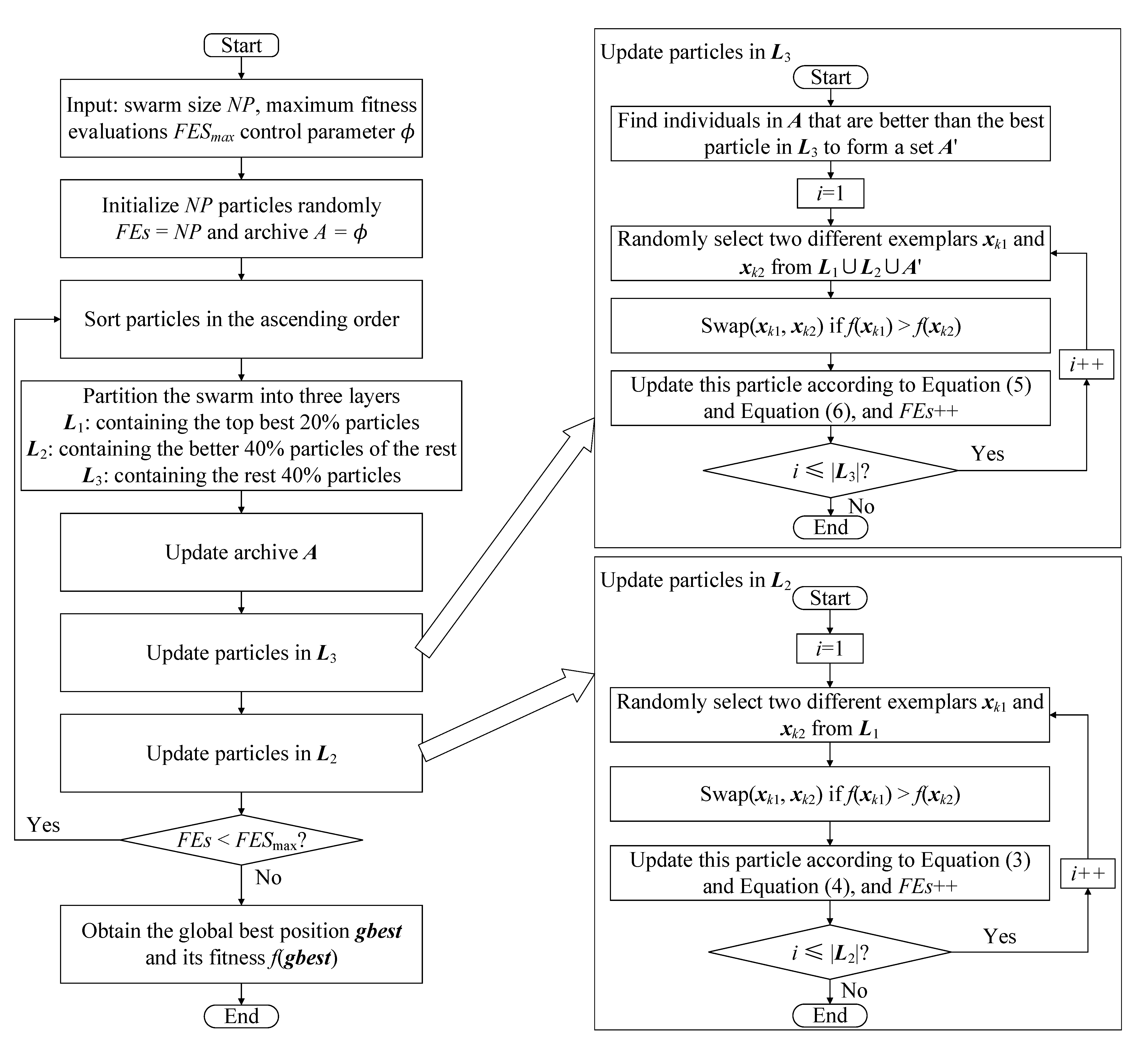
Integrating the above components, the complete EDPSO is obtained with its overall flowchart exhibited in Figure 1 and the overall procedure presented in Algorithm 1. Specifically, in the beginning, NP particles are randomly initialized and evaluated as shown in Line 1. After that, the algorithm jumps into the main iteration (Lines 3–25). During the iteration, the whole swarm is sorted in an ascending order of fitness (Line 4), and then the swarm is partitioned into three layers (Line 5) along with the update of the archive A (Line 6). Subsequently, particles in L3 are updated (Lines 7–16), following which is the update of particles in L2 (Lines 17–25). The main iteration proceeds until the maximum number of fitness evaluations is exhausted. Then, at the end of the algorithm, the global best position gbest and its fitness f(gbest) are obtained from L1 as the output.
From Algorithm 1, we can see that EDPSO needs O(NP × D) to store the positions of all particles and O(NP × D) to store the velocity of all particles. In addition, it also needs O(NP × D) to store the archive, and O(NP) to store the sorted index of particles. Comprehensively, EDPSO needs O(NP × D) space during the evolution.
Concerning the time complexity, in each generation, it takes O(NPlogNP) time to sort the swarm (Lines 4) and O(NP) to divide the swarm into three layers (Lines 5–6). Then, it takes O(NP × D) to update the archive (Lines 6), and to update particles in L2 and L3 (Lines 7–25) O(NP × D) time complexity is also needed. To sum up, the whole complexity in one generation is O(NP × D), which is the same as the classical PSO.
Algorithm 1: The pseudocode of EDPSO
Input: swarm size NP, maximum fitness evaluations FESmax and control parameter
1:Initialize NP particles randomly and caculate their fitness;
2:FEs = NP and set the archive empty A =
3:While (FEs < FESmax) do
4:  Sort particles in ascending order according to their fitness;
5:  Partition the swarm into three layers: the elite layer L1 containing the top best 20% of particles, the second layer L2 containing the half best of the non-elite particles (40% particles), and the third layer L3 consisting of another half of the non-elite particles (40% particles);
6:  Update the archive A;
7:  For each particle in L3 do
8:      Find those individuals in A that are better than the best particle in L3 to form a set A’;
9:      Select two different exemplars xk1 and xk2 from L1L2A’;
10:      If f(xk1) > f(xk2) then
11:         Swap(xk1, xk2);
12:      End If
13:      Update this particle according to Equations (4) and (5);
14:      If the elements in xi are smaller than the lower bounds of the associated variables, they are set as the asociated lower bounds; if they are larger than the upper bounds of the associated variables, they are set as the associated upper bounds.
15:      Evaluate its fitness and FEs++;
16:    End For
17:    For each particle in L2 do
18:      Select two different exemplars xk1 and xk2 from L1;
19:      If f(xk1) > f(xk2) then
20:         Swap(xk1, xk2);
21:      End If
22:      Update this particle according to Equations (6) and (7);
23:      If the elements in xi are smaller than the lower bounds of the associated variables, they are set as the asociated lower bounds; if they are larger than the upper bounds of the associated variables, they are set as the associated upper bounds.
24:      Evaluate its fitness and FEs++;
25:    End For
26:End While
27:Obtain the global best position gbest and its fitness f(gbest);
Output: f(gbest) and gbest

4. Experiments

In this section, we conduct extensive comparison experiments to validate the effectiveness of the proposed EDPSO on the commonly used CEC’2010 [58] and CEC’2013 [59] large-scale benchmark problem sets by comparing EDPSO with several state-of-the-art large-scale optimizers. The CEC’2010 set contains twenty 1000-D optimization problems, while the CEC’2013 set consists of fifteen 1000-D problems. In particular, the CEC’2013 set is an extension of the CEC’2010 set by introducing more complicated features, such as overlapping interacting variables and unbalanced contribution of variables. Therefore, the CEC’2013 benchmark problems are more difficult to optimize. The main characteristics of the CEC’2010 and the CEC’2013 sets are briefly summarized in Table 1 and Table 2, respectively. For more details, please refer to [58,59].
In this section, we first investigate the parameter settings of the swarm size NP and the control parameter ϕ for EDPSO in Section 4.1. Then, in Section 4.2, the proposed EDPSO is extensively compared with several state-of-the-art large-scale algorithms on the two benchmark sets. Lastly, in Section 4.3, the effectiveness of the additional archive in EDPSO is verified by conducting experiments on the CEC’2010 benchmark set.
In the experiments, for fair comparisons, without being otherwise stated, the maximum number of fitness evaluations is set as 3000 × D (where D is the dimension size) for all algorithms. For each algorithm on each optimization problem, we execute it independently for 30 runs, and then utilize the median, the mean, and the standard deviation (Std) values over the 30 independent runs to evaluate its performance, so that fair and comprehensive comparisons can be made.
In addition, to tell whether there is significant difference between the proposed EDPSO and the compared methods, we run the Wilcoxon rank-sum test at the significance level of “α = 0.05” to compare the performance of EDPSO with that of each compared algorithm on each problem. Furthermore, to compare the overall performance of different algorithms on one whole benchmark set, we also conduct the Friedman test at the significance level of “α = 0.05” on each benchmark set.

4.1. Parameter Settings

In the proposed EDPSO, two parameters, namely the swarm size NP and the control parameter ϕ, are needed to fine-tune. Therefore, to find suitable settings for these two parameters for EDPSO, we conduct experiments on the CEC’2010 set by varying NP from 500 to 1000, and ϕ from 0.1 to 0.9 for EDPSO. The comparison results among these settings are shown in Table 1. In particular, in this table, the best results among different settings of ϕ under the same setting of NP are highlighted in bold. The average rank of each configuration of ϕ under the same setting of NP obtained by the Friedman test is also presented in the last row of each part in Table 1.
From Table 3, we can obtain the following findings. (1) For different settings of NP, we find that when NP ranges from 500 to 800, the most suitable ϕ is 0.4; when it ranges from 900 to 1000, the most suitable ϕ is 0.3. This indicates that the setting of ϕ is not so closely related to NP. (2) Furthermore, we find that neither a too small ϕ nor a too large ϕ is suitable for EDPSO. This is because a too small ϕ decreases the influence of the second exemplar on the updated particle, leading to the updated particle greedily approaching the promising area where the first exemplar is located. In this case, once the first exemplar falls into local areas, the updated particle likely falls into local basins as well. Therefore, the algorithm likely encounters premature convergence. On the contrary, a too large ϕ increases the influence of the second exemplar, leading to the updated particle being dragged too far away from promising areas. In this situation, the convergence of the swarm slows down. (3) It is observed that a relatively large NP is preferred for EDPSO to achieve good performance. This is because a small NP cannot afford enough diversity for the algorithm to explore the solution space. However, a too large NP (such as NP = 900 or 1000) is not beneficial for EDPSO to achieve good performance because too high diversity is afforded, leading to that the convergence of the swarm slows down.
Based on the above observation, NP = 600 and ϕ = 0.4 are the recommended settings for the two parameters in EDPSO when solving 1000-D optimization problems.

4.2. Comparisons with State-of-the-Art Large-Scale Optimizers

This section conducts extensive comparison experiments to compare the proposed EDPSO with several state-of-art large-scale algorithms including five holistic large-scale PSO optimizers and four state-of-the-art CCEAs. Specifically, the five holistic large-scale optimizers are TPLSO [31], SPLSO [55], LLSO [54], CSO [29], and SLPSO [55], respectively, while the four CCEAs are DECC-GDG [69], DECC-DG [74], DECC-RDG [79], and DECC-RDG2 [74], respectively. In particular, we compare EDPSO with these algorithms on the 1000-D CEC’2010 and the 1000-D CEC’2013 large-scale benchmark sets.
Table 4 and Table 5 show the fitness comparison results between EDPSO and the nine compared algorithms on the CEC’2010 and the CEC’2013 benchmark sets, respectively. In these two tables, the symbol “+” above the p-value indicates that the proposed EDPSO is significantly superior to the associated compared algorithms on the corresponding problems, and the symbol “−” means that EDPSO is significantly inferior to the associated compared algorithms on the related problems, while the symbol “=” denotes that EDPSO achieves equivalent performance with the compared algorithms on the associated problems. Accordingly, “w/t/l” in the second to last rows of the two tables count the numbers of “+”, “=”, and “–”, respectively. In addition, the last rows of the two tables present the averaged ranks of all algorithms, which are obtained from the Friedman test.
From Table 4, the comparison results between EDPSO and the nine compared algorithms on the 20 1000-D CEC’2010 benchmark problems are summarized as follows:
(1)
From the perspective of the averaged ranks (shown in the last row) obtained by the Friedman test, EDPSO and LLSO achieve much smaller rank values than the other eight compared algorithms. This demonstrates that the proposed EDPSO and LLSO achieve significantly better performance on the CEC’2010 benchmark set than the other eight compared algorithms.
(2)
In view of the results (shown in the second to last row) obtained from the Wilcoxon rank-sum test, it is intuitively found that the proposed EDPSO is significantly better than the nine compared algorithms on at least 11 problems, and shows inferiority to them on at most eight problems. In particular, compared with the five holistic large-scale PSOs (namely TPLSO, SPLSO, LLSO, CSO, and SL-PSO), EDPSO shows significant dominance to them on 11, 12, 11, 15, and 12 problems, respectively, and only displays inferiority to them on eight, seven, eight, five, and eight problems, respectively. In comparison with the four CCEAs (namely, DECC-GDG, DECC-DG2, DECC-RDG, and DECC-RDG2), EDPSO significantly outperforms DECC-GDG on 17 problems, and significantly beats DECC-DG2, DECC-RDG, and DECC-RDG2 on all 15 problems.
From Table 5, we can draw the following conclusions with respect to the comparison results between the proposed EDPSO and the nine state-of-the-art compared methods on the 15 1000-D CEC’2013 benchmark problems:
(1)
In terms of the average rank values obtained from the Friedman test, the proposed EDPSO achieves a much smaller rank value than seven compared algorithms. This indicates that the proposed EDPSO achieves much better overall performance than them on such a difficult benchmark set. In particular, EDPSO achieves considerably similar performance with LLSO, but obtains slightly inferior performance to TPLSO.
(2)
With respect to the results obtained from the Wilcoxon rank-sum test, in comparison with the five holistic large-scale PSO variants, EDPSO significantly dominates SPLSO, CSO, and SL-PSO six, eight, and eight problems, respectively, and only exhibits inferiority to them in three, three, and four problems, respectively. Compared with LLSO, EDPSO achieves very competitive performance with it. However, in comparison with TPLSO, EDPSO shows slightly inferiority on this benchmark set. Competed with the four CCEAs, EDPSO presents significant superiority to them all on 12 problems and displays inferiority to them all on three problems.
The above experiments have demonstrated the effectiveness of the proposed EDPSO in solving high-dimensional problems. To further demonstrate its efficiency, we conduct experiments on the CEC’2010 and the CEC’2013 benchmark sets to investigate the convergence behavior comparisons between EDPSO and the compared algorithms. In these experiments, we set the maximum number of fitness evaluations as 5 × 10⁶ for all algorithms. Then, we record the global best fitness every 5 × 10⁵ fitness evaluations.
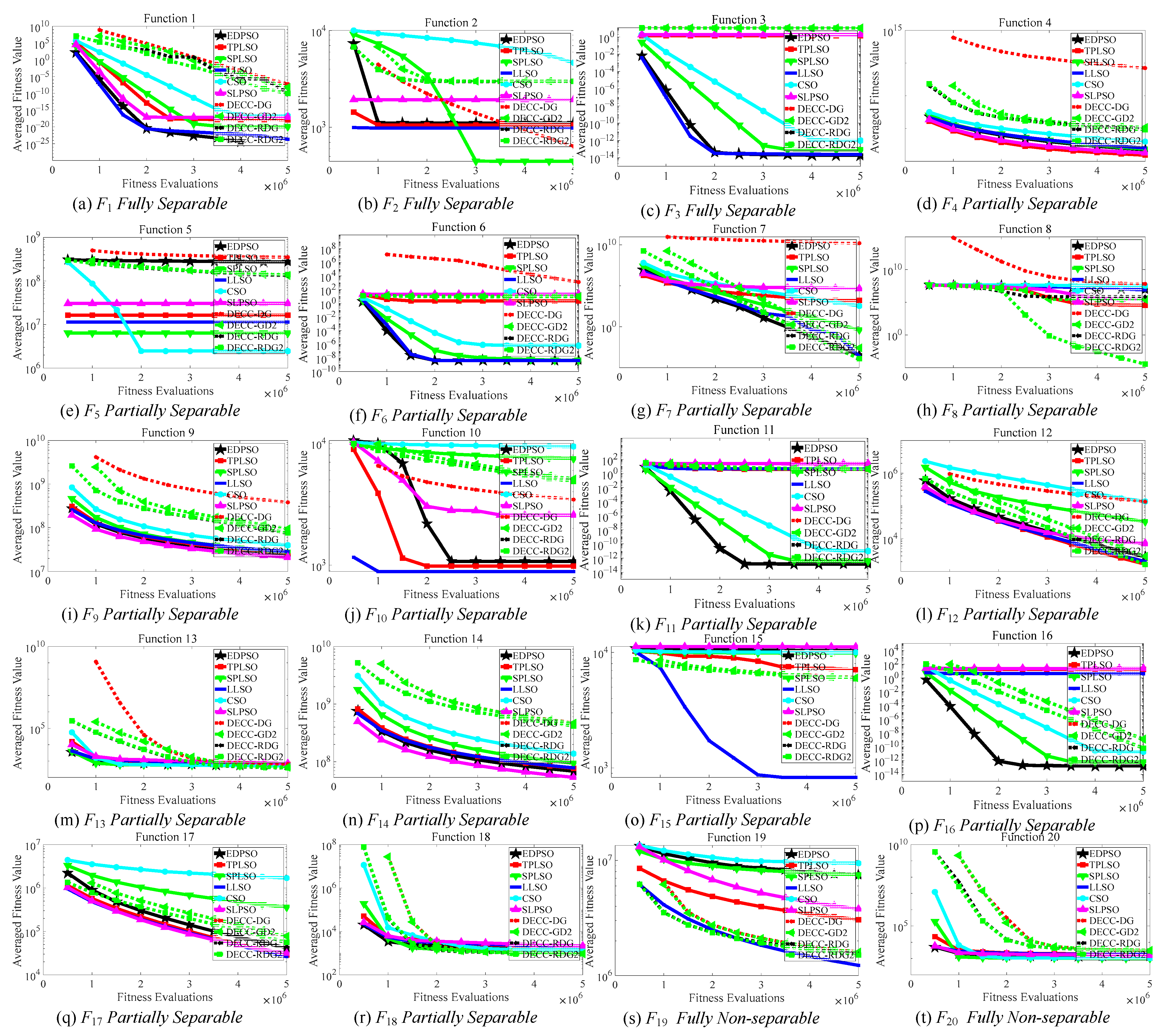
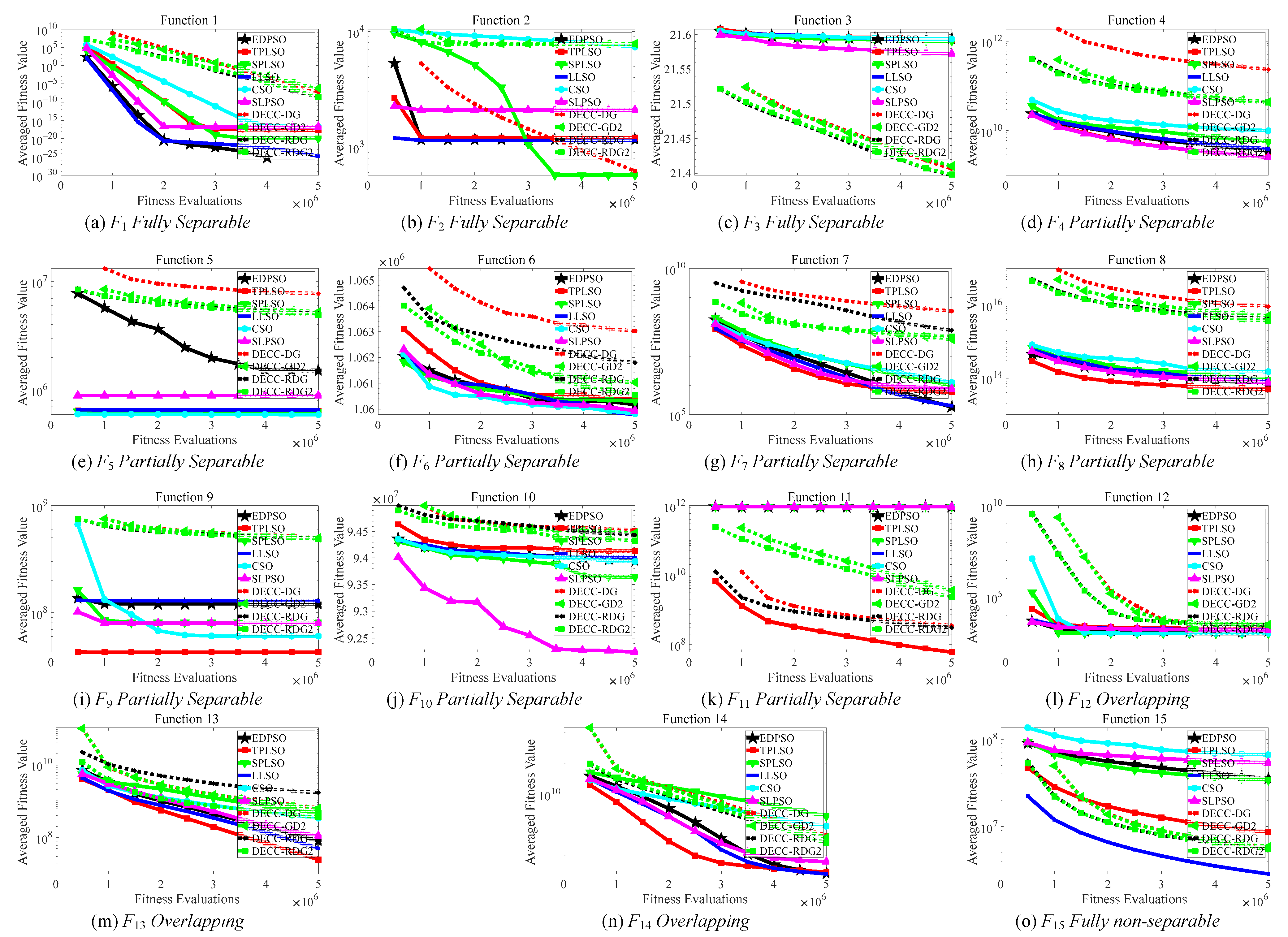
 Figure 2 and Figure 3 display the convergence behavior comparisons between EDPSO and the nine compared algorithms on the CEC’2010 and the CEC’2013 benchmark sets, respectively.
From Figure 2, at first glance, we find that EDPSO achieves clearly better performance than the nine compared algorithms in terms of both convergence speed and solution quality on three problems (F1, F11, and F16). In particular, EDPSO could finally find the true global optimum of F1. Taking deep observation, it is found that on the whole CEC’2010 benchmark set, the proposed EDPSO achieves highly competitive or even much better performance than most of the compared algorithms on most problems with respect to both the convergence speed and the solution quality. This implicitly demonstrates that the proposed EDPSO is efficient when solving high-dimensional problems.
From Figure 3, the convergence comparison results between the proposed EDPSO and the compared algorithms on the CEC’2013 show that the proposed EDPSO still presents considerably competitive or even great superiority to most of the compared algorithms on most problems in terms of both the convergence speed and the solution quality. This further demonstrates that the proposed EDPSO is efficient when solving complicated high-dimensional problems.
The above experiments on the two benchmark sets have demonstrated the effectiveness and efficiency of the proposed EDPSO. The superiority of EDPSO in solving high-dimensional problems mainly benefits from the proposed elite-directed learning strategy, which treats particles in different layers differently and lets particles in different layers learn from different numbers of predominant particles in higher layers. With this strategy, the learning effectiveness and the learning diversity of particles are largely improved, and the algorithm could compromise the search diversification and intensification well at the swarm level and the particle level to explore and exploit the solution space properly to obtain satisfactory performance.

4.3. Effectiveness of the Additional Archive

In this section, we conduct experiments to verify the usefulness of the additional archive. To this end, we first develop two versions of EDPSO. First, we remove the archive in EDPSO, leading to a variant of EDPSO, which we name as “EDPSO-WA”. Second, to demonstrate the effectiveness of using predominant individuals in the archive that are better than the best in the third layer, we replace this strategy by randomly choosing individuals in the archive along with the first two layers to direct the update of particles in the third layer. As a result, a new variant of EDPSO, which we name “EDPSO-ARand”, is developed. Then, we conduct experiments on the CEC’2010 benchmark set to compare the three different versions of EDPSO. Table 6 presents the comparison results with the best results in bold.
From Table 6, we can obtain the following findings. (1) With respect to the results of the Friedman test, the proposed EDPSO achieves the smallest rank among the three versions of EDPSO. In addition, from the perspective of the number of problems where the associated algorithm obtains the best results, we find the proposed EDPSO obtains the best results on 10 problems. These observations demonstrate the effectiveness of the additional archive and the way of using this archive. (2) Further, compared with EDPSO-WA, both the proposed EDPSO and EDPSO-ARand achieve much better performance. This demonstrates the usefulness of the additional archive. In comparison with EDPSO-ARand, the proposed EDPSO performs much better. This demonstrates the usefulness of the way of using predominant individuals in the archive to direct the update of particles in the third layer.
To summarize, the additional archive is helpful for EDPSO to achieve promising performance. This is because it introduces more candidate exemplars for particles in the third layer without destroying the convergence of the swarm. In this way, the learning diversity of particles is further promoted, which is beneficial for the swarm to explore the solution space and escape from local regions.

5. Conclusions

This paper has proposed an elite-directed particle swarm optimization with historical information (EDPSO) to tackle large-scale optimization problems. By taking inspiration from the “Pareto Principle”, which is also known as the 80-20 rule, we first partition the swarm into three layers with the first layer containing the top best 20% of particles and the other two layers of the same size consisting of the remaining 80% of particles. Then, particles in the third layer are updated by learning from two different exemplars randomly selected from those in the first two layers, and particles in the second layer are updated by learning from two different exemplars randomly selected from the first layer. To preserve the valuable evolutionary information, particles in the first layer are not updated and directly enter the next generation. To make full use of potentially valuable historical information, we additionally maintain an archive to store the obsolete elites in the first layer and then introduce them to the learning of particles in the third layer. With the above two techniques, particles in the last two layers could learn from different numbers of predominant candidates, and therefore the learning effectiveness and the learning diversity of particles are expectedly largely improved. By means of the proposed elite-directed learning strategy, EDPSO could compromise exploration and exploitation well at both the particle level and the swarm level to search high-dimensional space, which contributes to its promising performance solving complex large-scale optimization problems.
Extensive experiments have been conducted on the widely used CEC’2010 and CEC’2013 large-scale benchmark sets to validate the effectiveness of the proposed EDPSO. Experimental results have demonstrated that the proposed EDPSO could consistently achieve much better performance than the compared peer large-scale optimizers on the two benchmark sets. This verifies that EDPSO is promising for solving large-scale optimization problems in real-world applications.
However, in EDPSO, the control parameter ϕ is currently fixed and needs fine-tuning, which requires a lot of effort. To alleviate this issue, in the future, we will concentrate on devising an adaptive adjustment scheme for ϕ to eliminate its sensitivity based on the evolution state of the swarm and the evolutionary information of particles. In addition, to promote the application of the proposed EDPSO, in the future, we will also focus on utilizing EDPSO to solve real-world optimization problems.

Author Contributions

Q.Y.: Conceptualization, supervision, methodology, formal analysis, and writing—original draft preparation. Y.Z.: Implementation, formal analysis, and writing—original draft preparation. X.G.: Methodology, and writing—review, and editing. D.X.: Methodology, writing—review and editing. Z.L.: Writing—review and editing, and funding acquisition. All authors have read and agreed to the published version of the manuscript.

Funding

This work was supported in part by the National Natural Science Foundation of China under Grant 62006124 and U20B2061, in part by the Natural Science Foundation of Jiangsu Province under Project BK20200811, in part by the Natural Science Foundation of the Jiangsu Higher Education Institutions of China under Grant 20KJB520006, and in part by the Startup Foundation for Introducing Talent of NUIST.

Institutional Review Board Statement

Not applicable.

Informed Consent Statement

Not applicable.

Data Availability Statement

Not applicable.

Conflicts of Interest

The authors declare no conflict of interest.

References

  1. Lu, Z.; Liang, S.; Yang, Q.; Du, B. Evolving Block-Based Convolutional Neural Network for Hyperspectral Image Classification. IEEE Trans. Geosci. Remote Sens. 2022, 60, 1–21. [Google Scholar] [CrossRef]
  2. Chen, W.-N.; Tan, D.-Z.; Yang, Q.; Gu, T.; Zhang, J. Ant Colony Optimization for the Control of Pollutant Spreading on Social Networks. IEEE Trans. Cybern. 2019, 50, 4053–4065. [Google Scholar] [CrossRef] [PubMed]
  3. Yu, W.; Dillon, T.S.; Mostafa, F.; Rahayu, W.; Liu, Y. A Global Manufacturing Big Data Ecosystem for Fault Detection in Predictive Maintenance. IEEE Trans. Ind. Inform. 2019, 16, 183–192. [Google Scholar] [CrossRef]
  4. Kang, B.; Kim, D.; Choo, H. Internet of Everything: A Large-Scale Autonomic IoT Gateway. IEEE Trans. Multi-Scale Comput. Syst. 2017, 3, 206–214. [Google Scholar] [CrossRef]
  5. Dawaliby, S.; Bradai, A.; Pousset, Y. Distributed Network Slicing in Large Scale IoT Based on Coalitional Multi-Game Theory. IEEE Trans. Netw. Serv. Manag. 2019, 16, 1567–1580. [Google Scholar] [CrossRef]
  6. Mahdavi, S.; Shiri, M.E.; Rahnamayan, S. Metaheuristics in large-scale global continues optimization: A survey. Inf. Sci. 2015, 295, 407–428. [Google Scholar] [CrossRef]
  7. Omidvar, M.N.; Li, X.; Yao, X. A review of population-based metaheuristics for large-scale black-box global optimization: Part A. IEEE Trans. Evol. Comput. 2021, 1. [Google Scholar] [CrossRef]
  8. Omidvar, M.N.; Li, X.; Yao, X. A review of population-based metaheuristics for large-scale black-box global optimization: Part B. IEEE Trans. Evol. Comput. 2021, 1. [Google Scholar] [CrossRef]
  9. Hashim, F.A.; Houssein, E.H.; Mabrouk, M.S.; Al-Atabany, W.; Mirjalili, S. Henry gas solubility optimization: A novel physics-based algorithm. Futur. Gener. Comput. Syst. 2019, 101, 646–667. [Google Scholar] [CrossRef]
  10. Anita; Yadav, A. AEFA: Artificial electric field algorithm for global optimization. Swarm Evol. Comput. 2019, 48, 93–108. [Google Scholar] [CrossRef]
  11. Zeng, N.; Wang, Z.; Liu, W.; Zhang, H.; Hone, K.; Liu, X. A Dynamic Neighborhood-Based Switching Particle Swarm Optimization Algorithm. IEEE Trans. Cybern. 2020, 1–12. [Google Scholar] [CrossRef] [PubMed]
  12. Wang, X.; Zhang, K.; Wang, J.; Jin, Y. An Enhanced Competitive Swarm Optimizer with Strongly Convex Sparse Operator for Large-Scale Multi-Objective Optimization. IEEE Trans. Evol. Comput. 2021, 1. [Google Scholar] [CrossRef]
  13. Yang, Q.; Chen, W.-N.; Yu, Z.; Gu, T.; Li, Y.; Zhang, H.; Zhang, J. Adaptive Multimodal Continuous Ant Colony Optimization. IEEE Trans. Evol. Comput. 2016, 21, 191–205. [Google Scholar] [CrossRef] [Green Version]
  14. Abdelbar, A.M.; Salama, K.M. Parameter Self-Adaptation in an Ant Colony Algorithm for Continuous Optimization. IEEE Access 2019, 7, 18464–18479. [Google Scholar] [CrossRef]
  15. Liu, J.; Anavatti, S.; Garratt, M.; Abbass, H.A. Multi-operator continuous ant colony optimisation for real world problems. Swarm Evol. Comput. 2021, 69, 100984. [Google Scholar] [CrossRef]
  16. Mirjalili, S.; Gandomi, A.H.; Mirjalili, S.Z.; Saremi, S.; Faris, H.; Mirjalili, S.M. Salp swarm algorithm: A bio-inspired optimizer for engineering design problems. Adv. Eng. Softw. 2017, 114, 163–191. [Google Scholar] [CrossRef]
  17. Mirjalili, S.; Mirjalili, S.M.; Lewis, A. Grey Wolf Optimizer. Adv. Eng. Softw. 2014, 69, 46–61. [Google Scholar] [CrossRef] [Green Version]
  18. Bouchekara, H.R.E.H. Most Valuable Player Algorithm: A novel optimization algorithm inspired from sport. Oper. Res. 2020, 20, 139–195. [Google Scholar] [CrossRef]
  19. Abualigah, L.; Diabat, A.; Mirjalili, S.; Elaziz, M.A.; Gandomi, A.H. The Arithmetic Optimization Algorithm. Comput. Methods Appl. Mech. Eng. 2021, 376, 113609. [Google Scholar] [CrossRef]
  20. Mirjalili, S. SCA: A Sine Cosine Algorithm for solving optimization problems. Knowl. Based Syst. 2016, 96, 120–133. [Google Scholar] [CrossRef]
  21. Holland, J.H. Genetic algorithms. Sci. Am. 1992, 267, 66–73. [Google Scholar] [CrossRef]
  22. Yang, Q.; Xie, H.-Y.; Chen, W.-N.; Zhang, J. Multiple parents guided differential evolution for large scale optimization. In Proceedings of the 2016 IEEE Congress on Evolutionary Computation (CEC), Vancouver, BC, Canada, 24–29 July 2016; pp. 3549–3556. [Google Scholar]
  23. Yu, W.-J.; Ji, J.-Y.; Gong, Y.-J.; Yang, Q.; Zhang, J. A tri-objective differential evolution approach for multimodal optimization. Inf. Sci. 2018, 423, 1–23. [Google Scholar] [CrossRef]
  24. Li, G.; Meng, Z.; Hu, H. An adaptive hybrid approach for reliability-based design optimization. Struct. Multidiscip. Optim. 2014, 51, 1051–1065. [Google Scholar] [CrossRef]
  25. Heidari, A.A.; Mirjalili, S.; Faris, H.; Aljarah, I.; Mafarja, M.; Chen, H. Harris hawks optimization: Algorithm and applications. Futur. Gener. Comput. Syst. 2019, 97, 849–872. [Google Scholar] [CrossRef]
  26. Yang, Y.; Chen, H.; Heidari, A.A.; Gandomi, A.H. Hunger games search: Visions, conception, implementation, deep analysis, perspectives, and towards performance shifts. Expert Syst. Appl. 2021, 177, 114864. [Google Scholar] [CrossRef]
  27. Chopra, N.; Ansari, M.M. Golden jackal optimization: A novel nature-inspired optimizer for engineering applications. Expert Syst. Appl. 2022, 198, 116924. [Google Scholar] [CrossRef]
  28. Wang, Z.-J.; Zhan, Z.-H.; Yu, W.-J.; Lin, Y.; Zhang, J.; Gu, T.-L.; Zhang, J. Dynamic Group Learning Distributed Particle Swarm Optimization for Large-Scale Optimization and Its Application in Cloud Workflow Scheduling. IEEE Trans. Cybern. 2020, 50, 2715–2729. [Google Scholar] [CrossRef]
  29. Cheng, R.; Jin, Y. A Competitive Swarm Optimizer for Large Scale Optimization. IEEE Trans. Cybern. 2015, 45, 191–204. [Google Scholar] [CrossRef]
  30. Yang, Q.; Chen, W.-N.; Gu, T.; Jin, H.; Mao, W.; Zhang, J. An Adaptive Stochastic Dominant Learning Swarm Optimizer for High-Dimensional Optimization. IEEE Trans. Cybern. 2020, 52, 1960–1976. [Google Scholar] [CrossRef]
  31. Lan, R.; Zhu, Y.; Lu, H.; Liu, Z.; Luo, X. A Two-Phase Learning-Based Swarm Optimizer for Large-Scale Optimization. IEEE Trans. Cybern. 2020, 51, 6284–6293. [Google Scholar] [CrossRef]
  32. Kong, F.; Jiang, J.; Huang, Y. An Adaptive Multi-Swarm Competition Particle Swarm Optimizer for Large-Scale Optimization. Mathematics 2019, 7, 521. [Google Scholar] [CrossRef] [Green Version]
  33. Wang, H.; Liang, M.; Sun, C.; Zhang, G.; Xie, L. Multiple-strategy learning particle swarm optimization for large-scale optimization problems. Complex Intell. Syst. 2021, 7, 1–16. [Google Scholar] [CrossRef]
  34. Liang, J.; Chen, G.; Qu, B.; Yu, K.; Yue, C.; Qiao, K.; Qian, H. Cooperative co-evolutionary comprehensive learning particle swarm optimizer for formulation design of explosive simulant. Memetic Comput. 2020, 12, 331–341. [Google Scholar] [CrossRef]
  35. Li, X.; Yao, X. Cooperatively Coevolving Particle Swarms for Large Scale Optimization. IEEE Trans. Evol. Comput. 2012, 16, 210–224. [Google Scholar] [CrossRef]
  36. Goh, C.; Tan, K.; Liu, D.; Chiam, S. A competitive and cooperative co-evolutionary approach to multi-objective particle swarm optimization algorithm design. Eur. J. Oper. Res. 2010, 202, 42–54. [Google Scholar] [CrossRef]
  37. Song, G.-W.; Yang, Q.; Gao, X.-D.; Ma, Y.-Y.; Lu, Z.-Y.; Zhang, J. An Adaptive Level-Based Learning Swarm Optimizer for Large-Scale Optimization. In Proceedings of the 2021 IEEE International Conference on Systems, Man, and Cybernetics (SMC), Melbourne, Australia, 17–20 October 2021; pp. 152–159. [Google Scholar]
  38. Xie, H.-Y.; Yang, Q.; Hu, X.-M.; Chen, W.-N. Cross-generation Elites Guided Particle Swarm Optimization for large scale optimization. In Proceedings of the 2016 IEEE Symposium Series on Computational Intelligence (SSCI), Athens, Greece, 6–9 December 2016; pp. 1–8. [Google Scholar]
  39. Wang, Z.-J.; Zhan, Z.-H.; Kwong, S.; Jin, H.; Zhang, J. Adaptive Granularity Learning Distributed Particle Swarm Optimization for Large-Scale Optimization. IEEE Trans. Cybern. 2020, 51, 1175–1188. [Google Scholar] [CrossRef]
  40. Cheng, S.; Zhan, H.; Yao, H.; Fan, H.; Liu, Y. Large-scale many-objective particle swarm optimizer with fast convergence based on Alpha-stable mutation and Logistic function. Appl. Soft Comput. 2021, 99, 106947. [Google Scholar] [CrossRef]
  41. Wang, Q.; Zhang, L.; Wei, S.; Li, B.; Xi, Y. Tensor factorization-based particle swarm optimization for large-scale many-objective problems. Swarm Evol. Comput. 2021, 69, 100995. [Google Scholar] [CrossRef]
  42. Xu, B.; Zhang, Y.; Gong, D.; Guo, Y.; Rong, M. Environment Sensitivity-Based Cooperative Co-Evolutionary Algorithms for Dynamic Multi-Objective Optimization. IEEE/ACM Trans. Comput. Biol. Bioinform. 2018, 15, 1877–1890. [Google Scholar] [CrossRef]
  43. Ma, X.; Li, X.; Zhang, Q.; Tang, K.; Liang, Z.; Xie, W.; Zhu, Z. A Survey on Cooperative Co-Evolutionary Algorithms. IEEE Trans. Evol. Comput. 2019, 23, 421–441. [Google Scholar] [CrossRef]
  44. Potter, M.A.; De Jong, K.A. A cooperative coevolutionary approach to function optimization. In Parallel Problem Solving from Nature—PPSN III; Springer International Publishing: Berlin/Heidelberg, Germany, 1994; pp. 249–257. [Google Scholar]
  45. Yang, Z.; Tang, K.; Yao, X. Large scale evolutionary optimization using cooperative coevolution. Inf. Sci. 2008, 178, 2985–2999. [Google Scholar] [CrossRef] [Green Version]
  46. Bergh, F.V.D.; Engelbrecht, A. A Cooperative Approach to Particle Swarm Optimization. IEEE Trans. Evol. Comput. 2004, 8, 225–239. [Google Scholar] [CrossRef]
  47. Yang, Q.; Chen, W.-N.; Zhang, J. Evolution Consistency Based Decomposition for Cooperative Coevolution. IEEE Access 2018, 6, 51084–51097. [Google Scholar] [CrossRef]
  48. Omidvar, M.N.; Mei, Y.; Li, X. Effective decomposition of large-scale separable continuous functions for cooperative co-evolutionary algorithms. In Proceedings of the 2014 IEEE Congress on Evolutionary Computation (CEC), Beijing, China, 6–11 July 2014; pp. 1305–1312. [Google Scholar]
  49. Gong, D.; Xu, B.; Zhang, Y.; Guo, Y.; Yang, S. A Similarity-Based Cooperative Co-Evolutionary Algorithm for Dynamic Interval Multiobjective Optimization Problems. IEEE Trans. Evol. Comput. 2020, 24, 142–156. [Google Scholar] [CrossRef] [Green Version]
  50. Peng, X.; Liu, K.; Jin, Y. A dynamic optimization approach to the design of cooperative co-evolutionary algorithms. Knowl. Based Syst. 2016, 109, 174–186. [Google Scholar] [CrossRef]
  51. Meselhi, M.A.; Elsayed, S.M.; Sarker, R.A.; Essam, D.L. Contribution Based Co-Evolutionary Algorithm for Large-Scale Optimization Problems. IEEE Access 2020, 8, 203369–203381. [Google Scholar] [CrossRef]
  52. Yang, M.; Zhou, A.; Li, C.; Guan, J.; Yan, X. CCFR2: A more efficient cooperative co-evolutionary framework for large-scale global optimization. Inf. Sci. 2020, 512, 64–79. [Google Scholar] [CrossRef]
  53. Tian, Y.; Zheng, X.; Zhang, X.; Jin, Y. Efficient Large-Scale Multiobjective Optimization Based on a Competitive Swarm Optimizer. IEEE Trans. Cybern. 2019, 50, 3696–3708. [Google Scholar] [CrossRef] [Green Version]
  54. Yang, Q.; Chen, W.-N.; Da Deng, J.; Li, Y.; Gu, T.; Zhang, J. A Level-Based Learning Swarm Optimizer for Large-Scale Optimization. IEEE Trans. Evol. Comput. 2017, 22, 578–594. [Google Scholar] [CrossRef]
  55. Yang, Q.; Chen, W.-N.; Gu, T.; Zhang, H.; Deng, J.D.; Li, Y.; Zhang, J. Segment-Based Predominant Learning Swarm Optimizer for Large-Scale Optimization. IEEE Trans. Cybern. 2016, 47, 2896–2910. [Google Scholar] [CrossRef] [Green Version]
  56. Cheng, R.; Jin, Y. A social learning particle swarm optimization algorithm for scalable optimization. Inf. Sci. 2015, 291, 43–60. [Google Scholar] [CrossRef]
  57. Erridge, P. The Pareto Principle. Br. Dent. J. 2006, 201, 419. [Google Scholar] [CrossRef] [PubMed] [Green Version]
  58. Tang, K.; Li, X.; Suganthan, P.N.; Yang, Z.; Weise, T. Benchmark Functions for the CEC 2010 Special Session and Competition on Large-Scale Global Optimization; University of Science and Technology of China: Hefei, China, 2009. [Google Scholar]
  59. Li, X.; Tang, K.; Omidvar, M.N.; Yang, Z.; Qin, K. Benchmark Functions for the CEC 2013 Special Session and Competition on Large-Scale Global Optimization; Royal Melbourne Institute of Technology University: Melbourne, Australia, 2013. [Google Scholar]
  60. Kennedy, J.; Eberhart, R. Particle swarm optimization. In Proceedings of the International Conference on Neural Networks, Perth, WA, Australia, 27 November–1 December 1995; pp. 1942–1948. [Google Scholar]
  61. Zhan, Z.-H.; Zhang, J.; Li, Y.; Shi, Y.-H. Orthogonal Learning Particle Swarm Optimization. IEEE Trans. Evol. Comput. 2010, 15, 832–847. [Google Scholar] [CrossRef] [Green Version]
  62. Liang, J.J.; Qin, A.K.; Suganthan, P.N.; Baskar, S. Comprehensive learning particle swarm optimizer for global optimization of multimodal functions. IEEE Trans. Evol. Comput. 2006, 10, 281–295. [Google Scholar] [CrossRef]
  63. Lynn, N.; Ali, M.; Suganthan, P.N. Population topologies for particle swarm optimization and differential evolution. Swarm Evol. Comput. 2018, 39, 24–35. [Google Scholar] [CrossRef]
  64. Lin, A.; Sun, W.; Yu, H.; Wu, G.; Tang, H. Global genetic learning particle swarm optimization with diversity enhancement by ring topology. Swarm Evol. Comput. 2019, 44, 571–583. [Google Scholar] [CrossRef]
  65. Li, F.; Guo, J. Topology Optimization. In Advances in Swarm Intelligence; Springer International Publishing: Cham, Switzerland, 2014; pp. 142–149. [Google Scholar]
  66. Gong, Y.-J.; Li, J.-J.; Zhou, Y.; Li, Y.; Chung, H.S.-H.; Shi, Y.-H.; Zhang, J. Genetic Learning Particle Swarm Optimization. IEEE Trans. Cybern. 2015, 46, 2277–2290. [Google Scholar] [CrossRef] [Green Version]
  67. Romero, J.F.; Cotta, C. Optimization by Island-Structured Decentralized Particle Swarms. In Proceedings of the Computational Intelligence, Theory and Applications 2005; Springer: Berlin/Heidelberg, Germany, 2005; pp. 25–33. [Google Scholar]
  68. Liu, Y.; Yao, X.; Zhao, Q.; Higuchi, T. Scaling up fast evolutionary programming with cooperative coevolution. In Proceedings of the 2001 Congress on Evolutionary Computation (IEEE Cat. No.01TH8546), Seoul, Korea, 27–30 May 2001; pp. 1101–1108. [Google Scholar]
  69. Omidvar, M.N.; Li, X.; Mei, Y.; Yao, X. Cooperative Co-Evolution With Differential Grouping for Large Scale Optimization. IEEE Trans. Evol. Comput. 2014, 18, 378–393. [Google Scholar] [CrossRef] [Green Version]
  70. Zhang, X.; Du, K.-J.; Zhan, Z.-H.; Kwong, S.; Gu, T.-L.; Zhang, J. Cooperative Coevolutionary Bare-Bones Particle Swarm Optimization With Function Independent Decomposition for Large-Scale Supply Chain Network Design With Uncertainties. IEEE Trans. Cybern. 2019, 50, 4454–4468. [Google Scholar] [CrossRef]
  71. Yang, Q.; Chen, W.-N.; Gu, T.; Zhang, H.; Yuan, H.; Kwong, S.; Zhang, J. A Distributed Swarm Optimizer With Adaptive Communication for Large-Scale Optimization. IEEE Trans. Cybern. 2020, 50, 1–16. [Google Scholar] [CrossRef]
  72. Potter, M.A. The Design and Analysis of a Computational Model of Cooperative Coevolution; George Mason University: Fairfax, VA, USA, 1997. [Google Scholar]
  73. Ge, H.; Sun, L.; Tan, G.; Chen, Z.; Chen, C.L.P. Cooperative Hierarchical PSO With Two Stage Variable Interaction Reconstruction for Large Scale Optimization. IEEE Trans. Cybern. 2017, 47, 2809–2823. [Google Scholar] [CrossRef] [PubMed]
  74. Omidvar, M.N.; Yang, M.; Mei, Y.; Li, X.; Yao, X. DG2: A Faster and More Accurate Differential Grouping for Large-Scale Black-Box Optimization. IEEE Trans. Evol. Comput. 2017, 21, 929–942. [Google Scholar] [CrossRef] [Green Version]
  75. Yang, M.; Zhou, A.; Li, C.; Yao, X. An Efficient Recursive Differential Grouping for Large-Scale Continuous Problems. IEEE Trans. Evol. Comput. 2021, 25, 159–171. [Google Scholar] [CrossRef]
  76. Ma, X.; Huang, Z.; Li, X.; Wang, L.; Qi, Y.; Zhu, Z. Merged Differential Grouping for Large-scale Global Optimization. IEEE Trans. Evol. Comput. 2022, 1. [Google Scholar] [CrossRef]
  77. Xu, H.-B.; Li, F.; Shen, H. A Three-Level Recursive Differential Grouping Method for Large-Scale Continuous Optimization. IEEE Access 2020, 8, 141946–141957. [Google Scholar] [CrossRef]
  78. Liu, H.; Wang, Y.; Fan, N. A Hybrid Deep Grouping Algorithm for Large Scale Global Optimization. IEEE Trans. Evol. Comput. 2020, 24, 1112–1124. [Google Scholar] [CrossRef]
  79. Sun, Y.; Kirley, M.; Halgamuge, S.K. A Recursive Decomposition Method for Large Scale Continuous Optimization. IEEE Trans. Evol. Comput. 2018, 22, 647–661. [Google Scholar] [CrossRef]
  80. Sun, Y.; Omidvar, M.N.; Kirley, M.; Li, X. Adaptive threshold parameter estimation with recursive differential grouping for problem decomposition. In Proceedings of the Genetic and Evolutionary Computation Conference, Kyoto, Japan, 15–19 July 2018; pp. 889–896. [Google Scholar]
  81. Zhang, X.-Y.; Gong, Y.-J.; Lin, Y.; Zhang, J.; Kwong, S.; Zhang, J. Dynamic Cooperative Coevolution for Large Scale Optimization. IEEE Trans. Evol. Comput. 2019, 23, 935–948. [Google Scholar] [CrossRef]
  82. Yang, Q.; Zhang, K.-X.; Gao, X.-D.; Xu, D.-D.; Lu, Z.-Y.; Jeon, S.-W.; Zhang, J. A Dimension Group-Based Comprehensive Elite Learning Swarm Optimizer for Large-Scale Optimization. Mathematics 2022, 10, 1072. [Google Scholar] [CrossRef]
  83. Mohapatra, P.; Das, K.N.; Roy, S. A modified competitive swarm optimizer for large scale optimization problems. Appl. Soft Comput. 2017, 59, 340–362. [Google Scholar] [CrossRef]
  84. Deng, H.; Peng, L.; Zhang, H.; Yang, B.; Chen, Z. Ranking-based biased learning swarm optimizer for large-scale optimization. Inf. Sci. 2019, 493, 120–137. [Google Scholar] [CrossRef]
  85. Sheng, M.; Wang, Z.; Liu, W.; Wang, X.; Chen, S.; Liu, X. A particle swarm optimizer with multi-level population sampling and dynamic p-learning mechanisms for large-scale optimization. Knowl. Based Syst. 2022, 242, 108382. [Google Scholar] [CrossRef]
  86. Kampourakis, K. Understanding Evolution; Cambridge University Press: Cambridge, UK, 2014. [Google Scholar]
Figure 1. The overall flowchart of the proposed EDPSO.
Mathematics 10 01384 g001
Figure 2. Convergence behavior comparison between EDPSO and the compared algorithms on the 1000-D CEC’2010 functions.
Mathematics 10 01384 g002
Figure 3. Convergence behavior comparison between EDPSO and the compared algorithms on the 1000-D CEC’2013 functions.
Mathematics 10 01384 g003
Table 1. The main characteristics of the CEC’2010 functions.
FDimensionSeparabilityOptimaModality
F 1 1000fully separable0unimodal
F 2 1000fully separable0multimodal
F 3 1000fully separable0multimodal
F 4 1000partially separable0unimodal
F 5 1000partially separable0multimodal
F 6 1000partially separable0multimodal
F 7 1000partially separable0unimodal
1000partially separable0multimodal
F 9 1000partially separable0unimodal
1000partially separable0multimodal
F 11 1000partially separable0multimodal
F 12 1000partially separable0unimodal
F 13 1000partially separable0multimodal
F 14 1000partially separable0unimodal
1000partially separable0multimodal
F 16 1000partially separable0multimodal
F 17 1000partially separable0unimodal
F 18 1000partially separable0multimodal
F 19 1000fully non-separable0unimodal
F 20 1000fully non-separable0multimodal
Table 2. The main characteristics of the CEC’2013 functions.
FDimensionSeparabilityOptimaModality
F 1 1000fully separable0unimodal
F 2 1000fully separable0multimodal
F 3 1000fully separable0multimodal
F 4 1000partially separable0unimodal
F 5 1000partially separable0multimodal
F 6 1000partially separable0multimodal
F 7 1000partially separable0multimodal
F 8 1000partially separable0unimodal
F 9 1000partially separable0multimodal
F 10 1000partially separable0multimodal
F 11 1000partially separable0unimodal
F 12 1000overlapping0multimodal
F 13 905overlapping0unimodal
F 14 905overlapping0unimodal
F 15 1000fully non-separable0unimodal
Table 3. Comparison results of EDPSO with different settings of NP and ϕ on the 1000-D CEC’2010 problems with respect to the average fitness of the global best solutions found in 30 independent runs. In each part of this table with the same settings of NP, the best results obtained by EDPSO with the optimal ϕ are highlighted in bold.
FNP = 500FNP = 600
ϕ = 0.1ϕ = 0.2ϕ = 0.3ϕ = 0.4ϕ = 0.5ϕ = 0.6ϕ = 0.7ϕ = 0.8ϕ = 0.9ϕ = 0.1ϕ = 0.2ϕ = 0.3ϕ = 0.4ϕ = 0.5ϕ = 0.6ϕ = 0.7ϕ = 0.8ϕ = 0.9
F11.33 × 10−211.57 × 10−224.66 × 10−231.89 × 10−231.86 × 10−229.58 × 10−122.58 × 1022.83 × 1071.31 × 109F14.60 × 10−211.51 × 10−224.52 × 10−232.77 × 10−232.32 × 10−213.17 × 10−72.12 × 1048.43 × 1071.97 × 109
F21.23 × 1031.54 × 1031.72 × 1031.30 × 1039.12 × 1021.04 × 1041.08 × 1041.12 × 1041.19 × 104F21.02 × 1031.33 × 1031.32 × 1031.10 × 1032.66 × 1031.04 × 1041.07 × 1041.14 × 1041.19 × 104
F33.12 × 10−142.89 × 10−143.12 × 10−142.18 × 10−142.65 × 10−142.65 × 10−92.56 × 10−27.98 × 1001.55 × 101F34.43 × 10−142.65 × 10−143.01 × 10−142.18 × 10−143.60 × 10−146.21 × 10−74.36 × 10−11.05 × 1011.63 × 101
F45.36 × 10115.54 × 10113.89 × 10113.72 × 10112.43 × 10112.54 × 10114.07 × 10113.12 × 10138.64 × 1013F46.17 × 10115.52 × 10115.08 × 10114.14 × 10112.90 × 10112.28 × 10111.29 × 10124.35 × 10131.18 × 1014
F52.77 × 1082.85 × 1082.84 × 1082.94 × 1082.87 × 1082.85 × 1083.15 × 1083.22 × 1083.31 × 108F52.74 × 1082.86 × 1082.78 × 1082.85 × 1082.88 × 1082.94 × 1082.98 × 1082.98 × 1083.33 × 108
F64.00 × 10−96.71 × 1001.55 × 1014.00 × 10−94.00 × 10−94.03 × 10−85.59 × 10−29.28 × 1001.65 × 101F64.01 × 10−94.00 × 10−94.00 × 10−94.00 × 10−94.00 × 10−92.81 × 10−67.87 × 10−11.18 × 1011.74 × 101
F72.85 × 1013.19 × 1014.34 × 1014.86 × 1001.94 × 1006.72 × 1023.45 × 1042.42 × 1072.12 × 109F71.65 × 1028.34 × 1017.31 × 1017.50 × 1001.60 × 1012.85 × 1031.57 × 1058.17 × 1072.45 × 109
F83.01 × 1072.58 × 1072.40 × 1072.04 × 1072.16 × 1073.21 × 1074.14 × 1074.52 × 1074.66 × 107F83.31 × 1072.88 × 1072.70 × 1072.39 × 1072.58 × 1073.46 × 1074.25 × 1074.56 × 1074.65 × 107
F94.59 × 1075.19 × 1075.67 × 1073.95 × 1073.96 × 1078.27 × 1071.10 × 1091.47 × 10103.01 × 1010F94.87 × 1075.06 × 1075.41 × 1073.78 × 1074.15 × 1071.10 × 1083.69 × 1091.81 × 10103.50 × 1010
F101.23 × 1031.61 × 1031.63 × 1031.30 × 1039.83 × 1031.04 × 1041.08 × 1041.13 × 1041.17 × 104F109.20 × 1031.29 × 1031.39 × 1031.53 × 1031.02 × 1041.05 × 1041.08 × 1041.14 × 1041.19 × 104
F111.99 × 10−131.77 × 1012.03 × 1012.03 × 1011.61 × 10−133.54 × 10−76.75 × 10−14.56 × 1011.35 × 102F113.94 × 10−135.70 × 10−11.65 × 1011.54 × 10−132.82 × 10−131.41 × 10−54.62 × 1006.64 × 1011.49 × 102
F122.86 × 1041.98 × 1042.30 × 1041.07 × 1043.08 × 1042.05 × 1064.44 × 1065.47 × 1066.72 × 106F124.78 × 1042.47 × 1042.66 × 1041.73 × 1047.31 × 1042.99 × 1064.55 × 1065.63 × 1066.89 × 106
F138.24 × 1027.31 × 1027.46 × 1025.73 × 1025.53 × 1024.94 × 1028.23 × 1032.25 × 1075.95 × 109F137.83 × 1026.06 × 1026.05 × 1025.50 × 1025.17 × 1025.57 × 1027.41 × 1031.32 × 1081.09 × 1010
F141.31 × 1081.40 × 1081.57 × 1081.04 × 1081.12 × 1083.04 × 1085.87 × 1093.11 × 10105.53 × 1010F141.56 × 1081.45 × 1081.56 × 1081.17 × 1081.24 × 1085.06 × 1081.20 × 10103.80 × 10106.13 × 1010
F151.06 × 1041.08 × 1041.07 × 1041.06 × 1041.05 × 1041.06 × 1041.08 × 1041.13 × 1041.18 × 104F151.05 × 1041.05 × 1041.06 × 1041.06 × 1041.04 × 1041.05 × 1041.08 × 1041.13 × 1041.19 × 104
F161.48 × 1005.44 × 1006.67 × 1001.77 × 1002.93 × 10−18.78 × 10−88.68 × 10−11.66 × 1023.21 × 102F162.93 × 10−12.65 × 1001.51 × 1001.75 × 10−133.06 × 10−131.82 × 10−51.11 × 1012.18 × 1023.36 × 102
F172.33 × 1051.29 × 1051.31 × 1058.96 × 1045.05 × 1054.98 × 1068.44 × 1061.19 × 1071.48 × 107F174.51 × 1051.59 × 1051.46 × 1051.39 × 1052.11 × 1065.81 × 1069.40 × 1061.24 × 1071.50 × 107
F182.72 × 1033.54 × 1033.05 × 1032.04 × 1031.55 × 1032.76 × 1031.00 × 1056.35 × 1098.50 × 1010F182.01 × 1032.17 × 1033.00 × 1032.45 × 1031.58 × 1032.12 × 1033.91 × 1061.34 × 10109.69 × 1010
F199.54 × 1066.22 × 1066.10 × 1067.73 × 1061.09 × 1071.42 × 1071.70 × 1072.27 × 1072.53 × 107F191.03 × 1077.37 × 1066.84 × 1068.92 × 1061.14 × 1071.51 × 1071.95 × 1072.25 × 1072.64 × 107
F201.65 × 1032.05 × 1032.28 × 1031.53 × 1031.27 × 1031.25 × 1036.44 × 1046.85 × 1098.27 × 1010F201.75 × 1031.83 × 1031.94 × 1031.31 × 1031.18 × 1031.05 × 1033.89 × 1061.51 × 10101.08 × 1011
Rank3.53 4.15 4.43 2.452.55 4.50 6.45 7.95 9.00 Rank3.90 3.63 3.68 2.053.05 4.75 6.95 8.00 9.00
FNP = 700FNP = 800
ϕ = 0.1ϕ = 0.2ϕ = 0.3ϕ = 0.4ϕ = 0.5ϕ = 0.6ϕ = 0.7ϕ = 0.8ϕ = 0.9ϕ = 0.1ϕ = 0.2ϕ = 0.3ϕ = 0.4ϕ = 0.5ϕ = 0.6ϕ = 0.7ϕ = 0.8ϕ = 0.9
F18.23 × 10−182.92 × 10−226.67 × 10−237.69 × 10−233.84 × 10−184.62 × 10−41.92 × 1051.80 × 1082.84 × 109F13.60 × 10−146.27 × 10−221.10 × 10−224.98 × 10−223.99 × 10−147.53 × 10−29.19 × 1052.76 × 1083.52 × 109
F28.38 × 1021.18 × 1031.22 × 1039.67 × 1029.99 × 1031.03 × 1041.08 × 1041.14 × 1041.20 × 104F21.27 × 1031.02 × 1031.09 × 1038.38 × 1021.01 × 1041.05 × 1041.10 × 1041.14 × 1041.20 × 104
F32.42 × 10−122.77 × 10−142.65 × 10−142.29 × 10−141.60 × 10−122.38 × 10−52.07 × 1001.23 × 1011.68 × 101F31.76 × 10−102.89 × 10−142.89 × 10−142.65 × 10−141.69 × 10−103.43 × 10−43.48 × 1001.32 × 1011.72 × 101
F46.68 × 10118.31 × 10114.07 × 10114.72 × 10112.88 × 10113.39 × 10111.59 × 10123.88 × 10131.38 × 1014F45.44 × 10117.74 × 10116.56 × 10115.49 × 10114.23 × 10113.81 × 10112.15 × 10124.92 × 10131.09 × 1014
F52.81 × 1082.81 × 1082.84 × 1082.86 × 1082.78 × 1082.95 × 1083.00 × 1082.98 × 1083.15 × 108F52.76 × 1082.84 × 1082.80 × 1082.89 × 1082.89 × 1082.99 × 1082.92 × 1083.19 × 1083.25 × 108
F64.48 × 10−94.00 × 10−94.00 × 10−94.00 × 10−94.25 × 10−99.58 × 10−52.65 × 1001.34 × 1011.80 × 101F61.27 × 10−84.00 × 10−94.00 × 10−94.00 × 10−91.27 × 10−81.16 × 10−34.15 × 1001.42 × 1011.82 × 101
F74.12 × 1021.76 × 1022.47 × 1024.95 × 1011.06 × 1021.05 × 1045.97 × 1052.68 × 1083.69 × 109F71.55 × 1036.37 × 1021.08 × 1031.63 × 1023.23 × 1022.52 × 1041.04 × 1065.36 × 1084.64 × 109
F83.50 × 1073.12 × 1072.95 × 1072.69 × 1072.90 × 1073.62 × 1074.33 × 1074.54 × 1074.66 × 107F83.63 × 1073.30 × 1073.14 × 1072.92 × 1073.09 × 1073.76 × 1074.35 × 1074.59 × 1074.67 × 107
F96.27 × 1075.23 × 1075.25 × 1074.09 × 1074.73 × 1071.60 × 1086.71 × 1092.25 × 10103.59 × 1010F96.85 × 1075.83 × 1075.27 × 1074.63 × 1075.40 × 1072.63 × 1089.57 × 1092.40 × 10103.97 × 1010
F109.85 × 1031.16 × 1031.26 × 1033.79 × 1031.03 × 1041.06 × 1041.08 × 1041.14 × 1041.19 × 104F101.01 × 1041.02 × 1031.02 × 1039.96 × 1031.03 × 1041.05 × 1041.09 × 1041.15 × 1041.21 × 104
F116.45 × 10−111.49 × 10−131.45 × 10−131.41 × 10−135.30 × 10−114.23 × 10−49.31 × 1007.36 × 1011.57 × 102F113.81 × 10−91.42 × 10−131.35 × 10−131.41 × 10−134.52 × 10−95.26 × 10−31.56 × 1018.86 × 1011.65 × 102
F128.34 × 1043.22 × 1043.19 × 1042.56 × 1041.99 × 1053.38 × 1064.97 × 1066.12 × 1067.05 × 106F121.34 × 1054.03 × 1043.35 × 1043.69 × 1046.23 × 1053.43 × 1065.13 × 1066.09 × 1067.35 × 106
F136.12 × 1027.30 × 1027.43 × 1028.62 × 1025.05 × 1024.68 × 1025.39 × 1044.47 × 1081.33 × 1010F134.94 × 1026.67 × 1026.91 × 1027.08 × 1024.91 × 1024.72 × 1022.28 × 1058.72 × 1081.88 × 1010
F141.80 × 1081.52 × 1081.48 × 1081.14 × 1081.46 × 1089.38 × 1081.76 × 10104.20 × 10106.65 × 1010F142.13 × 1081.54 × 1081.55 × 1081.21 × 1081.85 × 1081.78 × 1092.40 × 10104.72 × 10106.86 × 1010
F151.05 × 1041.05 × 1041.05 × 1041.04 × 1041.03 × 1041.06 × 1041.10 × 1041.14 × 1041.19 × 104F151.04 × 1041.05 × 1041.05 × 1041.04 × 1041.04 × 1041.06 × 1041.10 × 1041.14 × 1041.21 × 104
F167.97 × 10−111.94 × 10−135.86 × 10−12.93 × 10−13.92 × 10−116.55 × 10−45.14 × 1012.49 × 1023.40 × 102F166.70 × 10−92.03 × 10−133.42 × 10−12.07 × 10−134.18 × 10−98.11 × 10−37.54 × 1012.66 × 1023.48 × 102
F171.02 × 1062.06 × 1051.75 × 1052.40 × 1052.77 × 1066.90 × 1069.55 × 1061.21 × 1071.61 × 107F172.33 × 1062.73 × 1052.10 × 1054.21 × 1053.90 × 1067.36 × 1069.71 × 1061.32 × 1071.55 × 107
F182.14 × 1032.57 × 1032.31 × 1031.77 × 1032.05 × 1032.62 × 1034.57 × 1072.28 × 10101.23 × 1011F181.97 × 1031.90 × 1032.13 × 1031.59 × 1031.20 × 1031.75 × 1032.35 × 1083.15 × 10101.43 × 1011
F191.16 × 1078.09 × 1067.83 × 1069.57 × 1061.17 × 1071.60 × 1072.00 × 1072.12 × 1072.69 × 107F191.22 × 1079.60 × 1068.07 × 1069.79 × 1061.25 × 1071.70 × 1071.97 × 1072.33 × 1072.90 × 107
F201.14 × 1031.69 × 1031.83 × 1031.34 × 1031.15 × 1031.01 × 1034.97 × 1072.36 × 10101.23 × 1011F201.15 × 1031.40 × 1031.67 × 1031.10 × 1031.03 × 1031.35 × 1032.81 × 1083.22 × 10101.42 × 1011
Rank4.00 3.13 3.15 2.483.05 5.20 7.05 7.95 9.00 Rank3.95 3.18 2.93 2.203.55 5.25 6.95 8.00 9.00
FNP = 900FNP = 1000
ϕ = 0.1ϕ = 0.2ϕ = 0.3ϕ = 0.4ϕ = 0.5ϕ = 0.6ϕ = 0.7ϕ = 0.8ϕ = 0.9ϕ = 0.1ϕ = 0.2ϕ = 0.3ϕ = 0.4ϕ = 0.5ϕ = 0.6ϕ = 0.7ϕ = 0.8ϕ = 0.9
F12.88 × 10−112.30 × 10−213.55 × 10−223.82 × 10−214.57 × 10−112.99 × 1002.72 × 1064.24 × 1084.36 × 109F15.39 × 10−97.77 × 10−201.84 × 10−211.08 × 10−181.13 × 10−84.65 × 1016.59 × 1065.75 × 1084.98 × 109
F28.01 × 1039.43 × 1029.92 × 1027.73 × 1021.02 × 1041.06 × 1041.09 × 1041.16 × 1041.21 × 104F29.60 × 1038.89 × 1029.57 × 1027.69 × 1031.02 × 1041.05 × 1041.10 × 1041.15 × 1041.22 × 104
F35.03 × 10−93.36 × 10−142.77 × 10−143.95 × 10−145.98 × 10−92.51 × 10−34.55 × 1001.40 × 1011.73 × 101F37.68 × 10−81.80 × 10−133.01 × 10−148.03 × 10−131.09 × 10−71.12 × 10−25.60 × 1001.45 × 1011.75 × 101
F47.99 × 10117.13 × 10116.84 × 10114.70 × 10114.30 × 10114.15 × 10114.18 × 10126.47 × 10131.52 × 1014F49.19 × 10119.07 × 10119.28 × 10116.61 × 10114.91 × 10115.14 × 10111.22 × 10137.49 × 10131.71 × 1014
F52.81 × 1082.87 × 1082.81 × 1082.88 × 1082.90 × 1082.96 × 1083.04 × 1083.21 × 1083.05 × 108F52.91 × 1082.87 × 1082.74 × 1082.91 × 1082.77 × 1082.90 × 1082.99 × 1083.24 × 1083.28 × 108
F68.16 × 10−84.00 × 10−94.00 × 10−94.00 × 10−98.88 × 10−87.56 × 10−35.51 × 1001.51 × 1011.86 × 101F67.90 × 10−74.11 × 10−94.00 × 10−94.20 × 10−99.85 × 10−73.28 × 10−26.85 × 1001.55 × 1011.89 × 101
F74.34 × 1031.64 × 1031.48 × 1036.09 × 1021.88 × 1034.68 × 1043.75 × 1066.39 × 1085.22 × 109F71.07 × 1046.59 × 1035.32 × 1031.33 × 1033.16 × 1037.82 × 1048.34 × 1061.06 × 1095.69 × 109
F83.75 × 1073.44 × 1073.30 × 1073.10 × 1073.26 × 1073.88 × 1074.40 × 1074.62 × 1074.67 × 107F83.84 × 1073.56 × 1073.42 × 1073.24 × 1073.40 × 1073.94 × 1074.42 × 1074.62 × 1074.67 × 107
F96.99 × 1075.67 × 1075.77 × 1074.59 × 1076.41 × 1075.03 × 1081.11 × 10102.51 × 10104.35 × 1010F98.37 × 1076.27 × 1076.76 × 1075.13 × 1077.33 × 1079.70 × 1081.28 × 10103.10 × 10104.55 × 1010
F101.01 × 1043.96 × 1031.69 × 1031.02 × 1041.03 × 1041.06 × 1041.10 × 1041.15 × 1041.22 × 104F101.02 × 1049.41 × 1039.35 × 1031.02 × 1041.03 × 1041.06 × 1041.09 × 1041.16 × 1041.22 × 104
F111.11 × 10−72.78 × 10−131.35 × 10−136.80 × 10−131.44 × 10−72.98 × 10−22.22 × 1011.03 × 1021.68 × 102F111.41 × 10−67.70 × 10−122.52 × 10−132.49 × 10−112.15 × 10−61.19 × 10−12.59 × 1011.09 × 1021.73 × 102
F122.26 × 1055.21 × 1044.08 × 1045.52 × 1041.33 × 1063.62 × 1064.90 × 1066.21 × 1067.22 × 106F123.83 × 1056.13 × 1044.93 × 1047.39 × 1041.72 × 1063.75 × 1065.27 × 1066.09 × 1067.39 × 106
F135.92 × 1027.06 × 1025.32 × 1026.44 × 1024.75 × 1024.77 × 1027.53 × 1051.59 × 1092.30 × 1010F135.02 × 1025.78 × 1025.37 × 1025.72 × 1025.23 × 1025.10 × 1022.54 × 1062.45 × 1092.90 × 1010
F142.41 × 1081.69 × 1081.68 × 1081.35 × 1082.46 × 1083.45 × 1092.75 × 10105.28 × 10107.32 × 1010F142.88 × 1081.80 × 1081.77 × 1081.50 × 1083.07 × 1085.52 × 1093.11 × 10105.41 × 10107.56 × 1010
F151.04 × 1041.04 × 1041.05 × 1041.04 × 1041.03 × 1041.06 × 1041.10 × 1041.15 × 1041.21 × 104F151.04 × 1041.03 × 1041.03 × 1041.03 × 1041.03 × 1041.07 × 1041.10 × 1041.16 × 1041.23 × 104
F161.16 × 10−72.77 × 10−131.97 × 10−134.64 × 10−131.43 × 10−76.00 × 10−29.28 × 1012.82 × 1023.51 × 102F161.75 × 10−64.05 × 10−122.67 × 10−131.78 × 10−112.51 × 10−62.39 × 10−11.19 × 1022.95 × 1023.58 × 102
F172.70 × 1063.51 × 1052.75 × 1058.26 × 1054.26 × 1067.45 × 1061.04 × 1071.33 × 1071.61 × 107F173.49 × 1065.20 × 1053.59 × 1051.52 × 1064.78 × 1067.70 × 1061.02 × 1071.29 × 1071.60 × 107
F181.28 × 1031.49 × 1032.04 × 1031.76 × 1031.22 × 1035.19 × 1036.05 × 1083.93 × 10101.71 × 1011F181.39 × 1031.82 × 1031.80 × 1031.51 × 1031.57 × 1037.40 × 1031.51 × 1094.85 × 10101.73 × 1011
F191.21 × 1079.49 × 1069.12 × 1061.06 × 1071.34 × 1071.66 × 1072.09 × 1072.27 × 1072.63 × 107F191.21 × 1079.70 × 1069.89 × 1061.08 × 1071.32 × 1071.60 × 1071.97 × 1072.35 × 1072.77 × 107
F201.13 × 1031.58 × 1031.73 × 1031.09 × 1031.03 × 1031.28 × 1036.96 × 1084.21 × 10101.67 × 1011F201.09 × 1031.15 × 1031.14 × 1039.99 × 1021.10 × 1034.70 × 1031.73 × 1095.17 × 10101.84 × 1011
Rank3.90 2.80 2.302.75 3.80 5.45 7.00 8.05 8.95 Rank3.95 2.90 2.252.55 3.85 5.50 7.00 8.00 9.00
Table 4. Fitness comparison between EDPSO and the compared algorithms on the 1000-D CEC’2010 problems with 3 × 10⁶ fitness evaluations with respect to the median, the mean, and the standard deviation values in the fitness of the global best solutions found in 30 independent runs. The symbols “+”, “−”, and “=” above the p-value indicate that EDPSO is significantly superior to, significantly inferior to, and equivalent to the compared algorithms on the associated problems. Those numbers in bold indicates that EDPSO performs significantly better than the compared algorithms.
FQualityEDPSOTPLSOSPLSOLLSOCSOSL_PSODECC_GDGDECC_DG2DECC_RDGDECC_RDG2
F1Median2.59 × 10−231.97 × 10−187.86 × 10−202.86 × 10−224.63 × 10−127.79 × 10−186.57 × 1001.95 × 10−12.60 × 10−31.05 × 10−3
Mean2.72 × 10−231.95 × 10−187.80 × 10−203.06 × 10−224.78 × 10−127.80 × 10−186.47 × 1007.70 × 10−16.42 × 1008.09 × 10−3
Std6.36 × 10−242.83 × 10−197.27 × 10−217.19 × 10−237.52 × 10−139.10 × 10−191.15 × 1001.64 × 1003.47 × 1013.33 × 10−2
p-value-3.02× 10⁻¹¹ +3.02 × 10⁻¹¹ +9.43 × 10⁻¹⁴ +3.02 × 10⁻¹¹ +3.02 × 10⁻¹¹ +3.02 × 10⁻¹¹ +3.02 × 10⁻¹¹ +3.02 × 10⁻¹¹ +3.02 × 10⁻¹¹ +
F2Median1.10 × 1031.10 × 1034.47 × 1029.72 × 1027.52 × 1031.94 × 1031.40 × 1032.99 × 1032.98 × 1033.00 × 103
Mean1.11 × 1031.11 × 1034.46 × 1029.85 × 1027.49 × 1031.94 × 1031.41 × 1033.02 × 1032.98 × 1033.01 × 103
Std4.97 × 1019.16 × 1011.65 × 1015.56 × 1012.54 × 1027.80 × 1012.36 × 1011.68 × 1021.18 × 1021.23 × 102
p-value-6.63 × 10−1 =3.01 × 10⁻¹¹ −1.16 × 10⁻¹⁰ −3.01 × 10⁻¹¹ +3.01 × 10⁻¹¹ +3.01 × 10⁻¹¹ +3.01 × 10⁻¹¹ +3.01 × 10⁻¹¹ +3.01 × 10⁻¹¹ +
F3Median2.18 × 10−141.43 × 1002.56 × 10−132.89 × 10−142.59 × 10−91.88 × 1001.13 × 1011.10 × 1011.12 × 1011.12 × 101
Mean2.20 × 10−141.44 × 1002.52 × 10−132.81 × 10−142.60 × 10−91.87 × 1001.13 × 1011.10 × 1011.11 × 1011.12 × 101
Std9.01 × 10−161.29 × 10−11.89 × 10−141.48 × 10−151.78 × 10−102.48 × 10−16.79 × 10−16.60 × 10−16.56 × 10−16.74 × 10⁻¹
p-value-2.36 × 10⁻¹² +2.27 × 10⁻¹² +1.49 × 10⁻¹⁴ +2.36 × 10⁻¹² +2.36 × 10⁻¹² +2.36 × 10⁻¹² +2.36 × 10⁻¹² +2.36 × 10⁻¹² +2.36 × 10⁻¹² +
F4Median3.92 × 10112.74 × 10114.38 × 10114.35 × 10116.95 × 10112.83 × 10111.39 × 10141.47 × 10121.39 × 10121.50 × 1012
Mean4.00 × 10112.95 × 10114.34 × 10114.46 × 10117.32 × 10112.91 × 10111.43 × 10141.73 × 10121.49 × 10121.49 × 1012
Std8.10 × 10108.68 × 10108.10 × 10101.16 × 10113.48 × 10119.25 × 10103.04 × 10136.33 × 10116.42 × 10115.54 × 1011
p-value-2.77 × 10⁻⁵ −5.55 × 10−2 =3.39 × 10⁻² +7.12 × 10⁻⁹ +3.57 × 10⁻⁶ −3.02 × 10⁻¹¹ +3.02 × 10⁻¹¹ +4.08 × 10⁻¹¹ +4.50 × 10⁻¹¹ +
F5Median2.84 × 1081.69 × 1075.97 × 1061.09 × 1072.00 × 1062.99 × 1073.85 × 1081.75 × 1081.74 × 1081.77 × 108
Mean2.82 × 1081.67 × 1076.37 × 1061.15 × 1072.49 × 1063.09 × 1073.83 × 1081.78 × 1081.71 × 1081.74 × 108
Std8.94 × 1064.65 × 1061.73 × 1062.58 × 1061.32 × 1068.58 × 1061.56 × 1071.96 × 1071.88 × 1071.62 × 107
p-value-3.02 × 10⁻¹¹ −2.76 × 10⁻¹¹ −9.23 × 10⁻¹⁴ −3.01 × 10⁻¹¹ −3.01 × 10⁻¹¹ −3.02 × 10⁻¹¹ +3.02 × 10⁻¹¹ −3.02 × 10⁻¹¹ −3.02 × 10⁻¹¹ −
F6Median4.00 × 10−92.07 × 1001.00 × 10−84.00 × 10−98.23 × 10−72.14 × 1013.55 × 1058.86 × 1001.06 × 1011.06 × 101
Mean4.00 × 10−92.22 × 1001.03 × 10−84.00 × 10−98.18 × 10−72.01 × 1013.65 × 1058.97 × 1001.05 × 1011.05 × 101
Std8.41 × 10−253.78 × 10−13.25 × 10−92.52 × 10−242.62 × 10−83.80 × 1004.61 × 1046.23 × 10−17.11 × 10−16.55 × 10−1
p-value-1.21 × 10⁻¹² +1.21 × 10⁻¹² +4.79 × 10⁻¹⁶ +1.21 × 10⁻¹² +1.21 × 10⁻¹² +1.21 × 10⁻¹² +1.21 × 10⁻¹² +1.21 × 10⁻¹² +1.21 × 10⁻¹² +
F7Median9.74 × 1009.00 × 1024.57 × 1028.37 × 1002.14 × 1046.29 × 1042.98 × 10101.84 × 1034.85 × 1015.23 × 101
Mean1.21 × 1016.02 × 1034.82 × 1024.22 × 1012.15 × 1046.57 × 1043.16 × 10102.03 × 1036.39 × 1015.94 × 101
Std6.14 × 1001.06 × 1041.26 × 1021.53 × 1024.51 × 1033.85 × 1044.44 × 1099.41 × 1024.74 × 1013.75 × 101
p-value-2.03 × 10−09 +3.02 × 10⁻¹¹ +1.54 × 10−1 =3.02 × 10⁻¹¹ +3.02 × 10⁻¹¹ +3.02 × 10⁻¹¹ +3.02 × 10⁻¹¹ +1.17 × 10⁻⁹ +2.61 × 10⁻¹⁰ +
F8Median2.41 × 1074.74 × 1053.11 × 1072.33 × 1073.86 × 1077.69 × 1066.98 × 1086.55 × 1026.56 × 10−14.30 × 10⁻¹
Mean2.41 × 1075.05 × 1053.11 × 1072.34 × 1073.87 × 1077.66 × 1068.24 × 1082.70 × 1056.64 × 1057.86 × 10−1
Std2.04 × 1051.43 × 1057.87 × 1042.45 × 1051.10 × 1052.47 × 1064.77 × 1081.01 × 1061.51 × 1061.26 × 100
p-value-3.02 × 10⁻¹¹ −3.02 × 10⁻¹¹ +2.15 × 10⁻¹³ −3.02 × 10⁻¹¹ +3.02 × 10⁻¹¹ −3.02 × 10⁻¹¹ +3.02 × 10⁻¹¹ −2.98 × 10⁻¹¹ −3.02 × 10⁻¹¹ −
F9Median3.99 × 1074.27 × 1074.66 × 1074.55 × 1076.72 × 1073.33 × 1077.56 × 1082.24 × 1081.76 × 1081.80 × 108
Mean3.94 × 1074.34 × 1074.62 × 1074.51 × 1076.70 × 1073.39 × 1077.46 × 1082.20 × 1081.73 × 1081.80 × 108
Std2.88 × 1064.39 × 1062.97 × 1064.04 × 1064.38 × 1063.82 × 1063.61 × 1071.82 × 1071.24 × 1071.76 × 107
p-value-2.39 × 10⁻⁴ +1.29 × 10⁻⁹ +1.43 × 10⁻⁸ +3.02 × 10⁻¹¹ +1.03 × 10⁻⁶ −3.02 × 10⁻¹¹ +3.02 × 10⁻¹¹ +3.02 × 10⁻¹¹ +3.02 × 10⁻¹¹ +
F10Median1.06 × 1039.70 × 1027.99 × 1038.92 × 1029.59 × 1032.59 × 1034.18 × 1036.75 × 1036.31 × 1036.29 × 103
Mean1.08 × 1039.77 × 1028.01 × 1038.87 × 1029.59 × 1032.82 × 1034.16 × 1036.73 × 1036.32 × 1036.30 × 103
Std5.90 × 1016.92 × 1011.17 × 1023.77 × 1016.49 × 1011.30 × 1035.47 × 1011.01 × 1021.14 × 1021.03 × 102
p-value-6.52 × 10⁻⁷ −3.02 × 10⁻¹¹ +9.41 × 10⁻¹⁴ −3.02 × 10⁻¹¹ +3.02 × 10⁻¹¹ +3.02 × 10⁻¹¹ +3.02 × 10⁻¹¹ +3.02 × 10⁻¹¹ +3.01 × 10⁻¹¹ +
F11Median1.51 × 10−133.51 × 1003.04 × 10−122.49 × 1003.97 × 10−82.43 × 1015.62 × 1005.44 × 1004.76 × 1004.86 × 100
Mean1.49 × 10−133.54 × 1003.07 × 10−124.60 × 1004.01 × 10−82.49 × 1015.63 × 1005.76 × 1004.75 × 1004.90 × 100
Std4.21 × 10−151.27 × 1002.73 × 10−134.80 × 1002.84 × 10−93.25 × 1005.50 × 10−17.71 × 10−14.88 × 10−13.79 × 10⁻¹
p-value-3.62 × 10⁻¹¹ +3.62 × 10⁻¹¹ +3.65 × 10⁻¹³ +3.62 × 10⁻¹¹ +3.62 × 10⁻¹¹ +3.62 × 10⁻¹¹ +3.62 × 10⁻¹¹ +3.62 × 10⁻¹¹ +3.62 × 10⁻¹¹ +
F12Median1.66 × 1041.18 × 1049.43 × 1041.23 × 1044.25 × 1051.29 × 1042.90 × 1054.04 × 1042.22 × 1042.21 × 104
Mean1.66 × 1041.20 × 1049.55 × 1041.23 × 1044.40 × 1051.54 × 1042.89 × 1053.98 × 1042.21 × 1042.21 × 104
Std1.21 × 1031.34 × 1036.73 × 1031.22 × 1036.21 × 1047.14 × 1031.05 × 1042.07 × 1031.30 × 1031.26 × 103
p-value-5.49 × 10⁻¹¹ −3.02 × 10⁻¹¹ +1.72 × 10⁻¹³ −3.02 × 10⁻¹¹ +4.51 × 10⁻² −3.02 × 10⁻¹¹ +3.02 × 10⁻¹¹ +3.34 × 10⁻¹¹ +3.02 × 10⁻¹¹ +
F13Median5.90 × 1027.42 × 1024.96 × 1027.81 × 1024.90 × 1028.91 × 1021.42 × 1031.67 × 1038.24 × 1028.27 × 102
Mean6.18 × 1027.57 × 1025.53 × 1028.21 × 1025.55 × 1029.88 × 1021.47 × 1031.84 × 1038.23 × 1028.49 × 102
Std1.62 × 1021.16 × 1021.67 × 1022.63 × 1021.77 × 1023.87 × 1023.57 × 1025.12 × 1021.38 × 1022.00 × 102
p-value-2.25 × 10⁻⁴ +5.94 × 10−2 =7.48 × 10⁻⁵ +8.50 × 10⁻² −7.60 × 10⁻⁷ +4.98 × 10⁻¹¹ +3.02 × 10⁻¹¹ +6.28 × 10⁻⁶ +2.88 × 10⁻⁶ +
F14Median1.09 × 1081.29 × 1081.61 × 1081.24 × 1082.48 × 1088.64 × 1078.61 × 1088.73 × 1087.18 × 1087.20 × 108
Mean1.08 × 1081.31 × 1081.61 × 1081.24 × 1082.48 × 1088.64 × 1078.67 × 1088.64 × 1087.23 × 1087.27 × 108
Std6.06 × 1061.39 × 1077.82 × 1067.66 × 1061.49 × 1077.53 × 1063.53 × 1073.91 × 1073.71 × 1073.44 × 107
p-value-1.61 × 10⁻¹⁰ +3.02 × 10⁻¹¹ +7.27 × 10⁻¹² +3.02 × 10⁻¹¹ +1.33 × 10⁻¹⁰ −3.02 × 10⁻¹¹ +3.02 × 10⁻¹¹ +3.02 × 10⁻¹¹ +3.02 × 10⁻¹¹ +
F15Median1.05 × 1041.01 × 1049.93 × 1038.33 × 1021.01 × 1041.12 × 1046.75 × 1036.74 × 1036.55 × 1036.58 × 103
Mean1.05 × 1048.70 × 1039.93 × 1038.72 × 1021.01 × 1041.13 × 1046.78 × 1036.75 × 1036.55 × 1036.57 × 103
Std7.80 × 1013.13 × 1035.23 × 1012.75 × 1026.55 × 1011.65 × 1029.92 × 1018.09 × 1019.01 × 1017.58 × 101
p-value-3.02 × 10⁻¹¹ −3.02 × 10⁻¹¹ −9.42 × 10⁻¹⁴ −3.01 × 10⁻¹¹−3.02 × 10⁻¹¹ +3.02 × 10⁻¹¹ −3.02 × 10⁻¹¹ −3.02 × 10⁻¹¹ −3.02 × 10⁻¹¹ −
F16Median1.76 × 10−131.72 × 1014.65 × 10−123.98 × 1005.69 × 10−82.28 × 1013.99 × 10−43.91 × 10−41.92 × 10−51.88 × 10⁻⁵
Mean1.77 × 10−131.88 × 1014.69 × 10−124.24 × 1005.74 × 10−82.47 × 1014.03 × 10−43.92 × 10−41.93 × 10−51.90 × 10⁻⁵
Std7.02 × 10−157.22 × 1004.46 × 10−132.08 × 1006.14 × 10−91.04 × 1012.55 × 10−51.34 × 10−59.05 × 10−78.73 × 10⁻⁷
p-value-2.90 × 10⁻¹¹ +1.93 × 10⁻³ +2.24 × 10⁻¹² +1.94 × 10⁻³ +2.90 × 10⁻¹¹ +1.94 × 10⁻³ +1.93 × 10⁻³ +2.76 × 10⁻¹¹ +2.76 × 10⁻¹¹ +
F17Median1.42 × 1059.72 × 1046.92 × 1059.15 × 1042.21 × 1062.97 × 1042.65 × 1052.65 × 1051.99 × 1051.97 × 105
Mean1.41 × 1059.71 × 1046.88 × 1059.17 × 1042.22 × 1063.21 × 1042.66 × 1052.65 × 1051.98 × 1051.99 × 105
Std8.66 × 1037.69 × 1033.42 × 1045.04 × 1032.10 × 1051.07 × 1047.98 × 1037.75 × 1038.87 × 1031.05 × 104
p-value-3.02 × 10⁻¹¹ −3.02 × 10⁻¹¹ +9.43 × 10⁻¹⁴ −3.02 × 10⁻¹¹ +3.02 × 10⁻¹¹ −3.02 × 10⁻¹¹ +3.02 × 10⁻¹¹ +3.02 × 10⁻¹¹ +3.02 × 10⁻¹¹ +
F18Median1.72 × 1032.27 × 1031.27 × 1032.51 × 1031.49 × 1032.01 × 1031.20 × 1031.16 × 1031.08 × 1031.12 × 103
Mean1.76 × 1032.33 × 1031.37 × 1032.56 × 1031.69 × 1032.19 × 1031.18 × 1031.15 × 1031.07 × 1031.12 × 103
Std3.45 × 1024.22 × 1023.77 × 1027.20 × 1028.08 × 1025.17 × 1021.38 × 1021.24 × 1021.09 × 1029.95 × 101
p-value-9.53 × 10⁻⁷ +3.83 × 10⁻⁶ −5.07 × 10⁻⁷ +3.78 × 10⁻² −1.37 × 10⁻³ +2.87 × 10⁻¹⁰ −1.09 × 10⁻¹⁰ −4.50 × 10⁻¹¹ −4.98 × 10⁻¹¹ −
F19Median8.66 × 1063.90 × 1068.22 × 1061.85 × 1069.80 × 1063.87 × 1062.14 × 1062.11 × 1061.96 × 1061.94 × 106
Mean8.57 × 1063.89 × 1068.26 × 1061.84 × 1069.88 × 1063.85 × 1062.15 × 1062.12 × 1061.95 × 1061.93 × 106
Std5.50 × 1052.71 × 1054.89 × 1058.65 × 1045.06 × 1055.38 × 1051.71 × 1051.05 × 1057.93 × 1049.83 × 104
p-value-3.02 × 10⁻¹¹ −4.36 × 10⁻² −9.43 × 10⁻¹⁴ −1.17 × 10⁻⁹ +3.02 × 10⁻¹¹ −3.02 × 10⁻¹¹ −3.02 × 10⁻¹¹ −3.02 × 10⁻¹¹ −3.02 × 10⁻¹¹ −
F20Median1.41 × 1032.00 × 1039.79 × 1021.96 × 1031.01 × 1031.59 × 1035.48 × 1035.42 × 1034.32 × 1034.29 × 103
Mean1.45 × 1032.05 × 1031.06 × 1031.95 × 1031.07 × 1031.59 × 1035.49 × 1035.50 × 1034.28 × 1034.37 × 103
Std1.69 × 1021.88 × 1021.78 × 1022.64 × 1021.72 × 1021.53 × 1023.52 × 1023.38 × 1022.34 × 1023.18 × 102
p-value-6.70 × 10⁻¹¹ +1.20 × 10⁻⁸ −9.59 × 10⁻¹² +3.49 × 10⁻⁹ −1.30 × 10⁻³ +3.02 × 10⁻¹¹ +3.02 × 10⁻¹¹ +3.02 × 10⁻¹¹ +3.02 × 10⁻¹¹ +
w/t/l11/1/8 12/1/711/1/815/0/5 12/0/817/0/3 15/0/5 15/0/5 15/0/5
Rank3.654.554.43.456.15.457.86.57.87.8
Table 5. Fitness comparison between EDPSO and the compared algorithms on the 1000-D CEC’2013 problems with 3 × 10⁶ fitness evaluations with respect to the median, the mean, and the standard deviation values in the fitness of the global best solutions found in 30 independent runs. The symbols “+”, “−”, and “=” above the p-value indicate that EDPSO is significantly superior to, significantly inferior to, and equivalent to the compared algorithms on the associated problems. Those numbers in bold indicates that EDPSO performs significantly better than the compared algorithms.
FQualityEDPSOTPLSOSPLSOLLSOCSOSL_PSODECC_GDGDECC_DG2DECC_RDGDECC_RDG2
F1Median4.19 × 10−233.04 × 10−181.18 × 10−194.10 × 10−228.07 × 10−121.03 × 10−177.13 × 1004.42 × 1002.39 × 10−23.09 × 10⁻²
Mean4.43 × 10−233.74 × 10−181.21 × 10−194.57 × 10−227.94 × 10−121.65 × 10−177.59 × 1007.11 × 1003.87 × 10−21.11 × 10⁻¹
Std1.26 × 10−231.64 × 10−181.21 × 10−201.69 × 10−221.23 × 10−123.30 × 10−171.03 × 1007.73 × 1003.97 × 10−22.12 × 10⁻¹
p-value-3.02 × 10⁻¹¹ +3.02 × 10⁻¹¹ +3.02 × 10⁻¹¹ +3.02 × 10⁻¹¹ +3.02 × 10⁻¹¹ +3.02 × 10⁻¹¹ +3.02 × 10⁻¹¹ +3.02 × 10⁻¹¹ +5.57 × 10⁻¹⁰ +
F2Median1.15 × 1031.23 × 1039.92 × 1021.14 × 1038.61 × 1032.13 × 1031.43 × 1037.85 × 1037.90 × 1037.87 × 103
Mean1.15 × 1031.23 × 1031.11 × 1031.15 × 1038.59 × 1032.14 × 1031.44 × 1037.92 × 1037.79 × 1037.78 × 103
Std5.03 × 1015.85 × 1014.74 × 1024.54 × 1011.84 × 1021.48 × 1022.18 × 1014.07 × 1023.64 × 1023.65 × 102
p-value-3.83 × 10⁻⁶ +8.50 × 10−2 =8.88 × 10−1 =3.01 × 10⁻¹¹ +3.01 × 10⁻¹¹ +3.01 × 10⁻¹¹ +3.01 × 10⁻¹¹ +3.01 × 10⁻¹¹ +3.01 × 10⁻¹¹ +
F3Median2.16 × 1012.16 × 1012.16 × 1012.16 × 1012.16 × 1012.16 × 1012.15 × 1012.15 × 1012.14 × 1012.15 × 101
Mean2.16 × 1012.16 × 1012.16 × 1012.16 × 1012.16 × 1012.16 × 1012.15 × 1012.15 × 1012.14 × 1012.15 × 101
Std5.79 × 10−32.34 × 10−22.60 × 10−26.00 × 10−31.78 × 10−23.02 × 10−21.10 × 10−21.22 × 10−21.11 × 10−28.29 × 10⁻³
p-value-3.22 × 10−1 =4.78 × 10−1 =4.33 × 10−1 =1.20 × 10−1 =3.50 × 10⁻³ +2.98 × 10⁻¹¹ −2.98 × 10⁻¹¹ −3.00 × 10⁻¹¹ −2.96 × 10⁻¹¹ −
F4Median6.11 × 1094.27 × 1099.23 × 1096.53 × 1091.25 × 10104.47 × 1094.19 × 10118.21 × 10107.84 × 10106.62 × 1010
Mean6.05 × 1094.28 × 1099.60 × 1096.68 × 1091.37 × 10104.46 × 1094.30 × 10118.02 × 10107.46 × 10106.92 × 1010
Std1.08 × 1091.06 × 1091.70 × 1091.50 × 1093.22 × 1098.94 × 1088.20 × 10102.22 × 10101.92 × 10102.32 × 1010
p-value-5.60 × 10⁻⁷ −2.15 × 10⁻¹⁰ +1.02 × 10−1 =3.02 × 10⁻¹¹ +6.05 × 10⁻⁷ −3.02 × 10⁻¹¹ +3.02 × 10⁻¹¹ +3.02 × 10⁻¹¹ +3.02 × 10⁻¹¹ +
F5Median6.96 × 1056.51 × 1056.48 × 1056.72 × 1056.08 × 1058.89 × 1058.66 × 1066.10 × 1065.85 × 1065.77 × 106
Mean1.97 × 1066.70 × 1056.40 × 1056.73 × 1056.09 × 1058.98 × 1058.70 × 1066.07 × 1065.78 × 1065.71 × 106
Std2.70 × 1061.02 × 1059.32 × 1049.47 × 1041.04 × 1051.27 × 1053.10 × 1052.21 × 1053.91 × 1053.58 × 105
p-value-4.92 × 10−1 =1.45 × 10−1 =5.89 × 10−1 =3.64 × 10⁻² −4.71 × 10⁻⁴ −3.02 × 10⁻¹¹ +6.76 × 10⁻⁵ +6.77 × 10⁻⁵ +6.77 × 10⁻⁵ +
F6Median1.06 × 1061.06 × 1061.06 × 1061.06 × 1061.06 × 1061.06 × 1061.06 × 1061.06 × 1061.06 × 1061.06 × 106
Mean1.06 × 1061.06 × 1061.06 × 1061.06 × 1061.06 × 1061.06 × 1061.06 × 1061.06 × 1061.06 × 1061.06 × 106
Std1.07 × 1032.34 × 1031.83 × 1031.17 × 1031.09 × 1032.23 × 1031.38 × 1031.43 × 1031.25 × 1031.23 × 103
p-value-4.20 × 10⁻⁴ +5.84 × 10−1 =4.38 × 10−1 =7.67 × 10−1 =4.87 × 10−1 =1.92 × 10⁻⁹ +5.11 × 10⁻⁴ +5.73 × 10⁻⁸ +6.96 × 10−05 +
F7Median2.53 × 1061.17 × 1065.52 × 1061.70 × 1065.56 × 1061.49 × 1067.74 × 1087.36 × 1072.93 × 1088.65 × 107
Mean2.70 × 1061.21 × 1065.61 × 1061.89 × 1065.98 × 1061.76 × 1067.94 × 1087.82 × 1073.76 × 1088.36 × 107
Std1.14 × 1064.52 × 1052.25 × 1061.07 × 1063.08 × 1061.51 × 1061.21 × 1082.80 × 1072.67 × 1082.05 × 107
p-value-3.65 × 10⁻⁸ −1.07 × 10⁻⁷ +1.77 × 10⁻³ −7.12 × 10⁻⁹ +2.00 × 10⁻⁵ +3.02 × 10⁻¹¹ +3.02 × 10⁻¹¹ +3.02 × 10⁻¹¹ +3.02 × 10⁻¹¹ +
F8Median1.20 × 10146.91 × 10131.59 × 10141.37 × 10142.45 × 10149.65 × 10131.74 × 10169.53 × 10156.96 × 10156.01 × 1015
Mean1.19 × 10147.19 × 10131.59 × 10141.38 × 10142.50 × 10141.11 × 10141.78 × 10169.38 × 10157.03 × 10156.58 × 1015
Std3.47 × 10133.55 × 10132.76 × 10133.45 × 10138.60 × 10135.49 × 10135.51 × 10152.73 × 10151.57 × 10152.08 × 1015
p-value-3.52 × 10⁻⁷ −1.25 × 10⁻⁵ +1.63 × 10⁻² +5.46 × 10⁻⁹ +1.22 × 10⁻¹ +3.02 × 10⁻¹¹ +3.02 × 10⁻¹¹ +3.02 × 10⁻¹¹ +3.02 × 10⁻¹¹ +
F9Median1.13 × 1084.33 × 1077.93 × 1071.13 × 1086.11 × 1078.10 × 1075.73 × 1085.58 × 1085.43 × 1085.36 × 108
Mean1.21 × 1084.23 × 1078.27 × 1071.47 × 1086.28 × 1078.11 × 1075.66 × 1085.62 × 1085.42 × 1085.34 × 108
Std3.29 × 1076.71 × 1062.18 × 1071.61 × 1081.31 × 1071.09 × 1073.06 × 1073.28 × 1073.02 × 1072.38 × 107
p-value-3.02 × 10⁻¹¹ −3.09 × 10⁻⁶ −8.07 × 10−1 =2.15 × 10⁻¹⁰ −9.06 × 10⁻⁸ −3.02 × 10⁻¹¹ +3.02 × 10⁻¹¹ +3.02 × 10⁻¹¹ +3.02 × 10⁻¹¹ +
F10Median9.41 × 1079.42 × 1079.40 × 1079.42 × 1079.41 × 1079.37 × 1079.47 × 1079.46 × 1079.47 × 1079.46 × 107
Mean9.41 × 1079.42 × 1079.40 × 1079.43 × 1079.41 × 1079.29 × 1079.46 × 1079.46 × 1079.46 × 1079.46 × 107
Std2.69 × 1052.77 × 1052.91 × 1053.26 × 1052.68 × 1051.55 × 1062.03 × 1052.51 × 1051.84 × 1052.47 × 105
p-value-9.93 × 10−02 =1.26 × 10−1 =3.27 × 10⁻² +7.06 × 10−1 =1.41 × 10⁻⁴ −3.16 × 10⁻¹⁰ +2.44 × 10⁻⁹ +9.91 × 10⁻¹¹ +5.96 × 10⁻⁹ +
F11Median9.26 × 10111.79 × 1089.23 × 10119.27 × 10119.35 × 10119.39 × 10116.93 × 1082.09 × 10105.84 × 1081.43 × 1010
Mean9.29 × 10111.78 × 1089.29 × 10119.31 × 10119.30 × 10119.36 × 10117.01 × 1082.68 × 10105.81 × 1081.52 × 1010
Std1.00 × 10105.06 × 1071.04 × 10101.08 × 10109.36 × 1098.27 × 1091.09 × 1081.48 × 10108.79 × 1077.61 × 109
p-value-3.02 × 10⁻¹¹ −8.42 × 10−1 =5.01 × 10⁻¹ −9.12 × 10−1 =1.17 × 10⁻² +3.02 × 10⁻¹¹ −3.02 × 10⁻¹¹ −3.02 × 10⁻¹¹ −3.02 × 10⁻¹¹ −
F12Median1.43 × 1032.03 × 1031.03 × 1031.82 × 1031.05 × 1031.76 × 1035.56 × 1035.51 × 1034.31 × 1034.32 × 103
Mean1.43 × 1032.04 × 1031.06 × 1031.84 × 1031.09 × 1031.78 × 1035.54 × 1035.63 × 1034.37 × 1034.33 × 103
Std8.89 × 1012.38 × 1025.91 × 1011.62 × 1028.43 × 1011.74 × 1023.77 × 1027.69 × 1023.24 × 1022.68 × 102
p-value-3.02 × 10⁻¹¹ +4.45 × 10⁻¹¹ −5.49 × 10⁻¹¹ +6.69 × 10⁻¹¹ −6.12 × 10⁻¹⁰ +3.02 × 10⁻¹¹ +3.02 × 10⁻¹¹ +3.02 × 10⁻¹¹ +3.02 × 10⁻¹¹ +
F13Median4.28 × 1081.84 × 1081.22 × 1093.07 × 1087.21 × 1084.03 × 1081.59 × 1091.47 × 1092.97 × 1097.15 × 108
Mean4.40 × 1082.12 × 1081.24 × 1093.45 × 1087.66 × 1086.26 × 1081.57 × 1091.54 × 1093.08 × 1097.23 × 108
Std1.50 × 1081.17 × 1085.06 × 1081.44 × 1082.87 × 1088.23 × 1083.45 × 1083.47 × 1088.07 × 1081.58 × 108
p-value-1.87 × 10⁻⁷ −6.12 × 10⁻¹⁰ +1.27 × 10⁻² −7.09 × 10⁻⁸ +7.06 × 10−1 =3.02 × 10⁻¹¹ +3.02 × 10⁻¹¹ +3.02 × 10⁻¹¹ +9.83 × 10⁻⁸ +
F14Median2.01 × 1085.81 × 1075.19 × 1099.27 × 1072.92 × 1091.56 × 1084.54 × 1094.83 × 1092.22 × 1093.09 × 109
Mean3.67 × 1085.98 × 1078.36 × 1091.61 × 1083.74 × 1092.71 × 1085.45 × 1094.71 × 1092.87 × 1093.43 × 109
Std4.23 × 1081.28 × 1076.66 × 1092.30 × 1083.35 × 1092.36 × 1083.96 × 1091.80 × 1091.90 × 1092.07 × 109
p-value-1.35 × 10⁻¹⁰ −4.46 × 10⁻¹¹ +9.45 × 10⁻⁵ −4.94 × 10⁻¹¹ +2.92 × 10−1 =8.20 × 10⁻¹¹ +8.20 × 10⁻¹¹ +3.29 × 10⁻¹⁰ +1.49 × 10⁻¹⁰ +
F15Median4.53 × 1071.24 × 1074.13 × 1074.63 × 1067.62 × 1076.06 × 1078.70 × 1068.92 × 1067.89 × 1068.03 × 106
Mean4.70 × 1071.23 × 1074.19 × 1074.63 × 1067.64 × 1076.10 × 1079.05 × 1069.08 × 1068.05 × 1068.16 × 106
Std7.77 × 1069.89 × 1053.55 × 1063.38 × 1056.06 × 1066.32 × 1069.14 × 1059.03 × 1051.01 × 1061.02 × 106
p-value-3.02 × 10⁻¹¹ −5.57 × 10⁻³ −3.02 × 10⁻¹¹ −3.69 × 10⁻¹¹ +4.31 × 10⁻⁸ +3.02 × 10⁻¹¹ −3.02 × 10⁻¹¹ −3.02 × 10⁻¹¹ −3.02 × 10⁻¹¹ −
w/t/l4/3/8 6/6/3 4/6/58/4/3 8/3/4 12/0/312/0/3 12/0/312/0/3
Rank4.07 3.53 4.73 4.00 5.53 4.40 8.20 7.60 6.80 6.13
Table 6. Fitness comparison between EDPSO with and without the archive on the 1000-D CEC’2010 problems with 3 × 10⁶ fitness evaluations with respect to the mean fitness of the global best solutions found in 30 independent runs. The best results are highlighted in bold.
FEDPSOEDPSO-WAEDPSO-ARand
F12.72 × 10−232.25 × 10−203.13 × 10⁻¹⁸
F21.11 × 1031.25 × 1037.58 × 102
F32.20 × 10−146.82 × 10−141.46 × 10⁻¹²
F44.00 × 10117.43 × 10113.36 × 1011
F52.82 × 1082.91 × 1082.73 × 108
F64.00 × 10−94.31 × 10−94.76 × 10−9
F71.21 × 1011.32 × 1041.99 × 104
F82.41 × 1073.53 × 1073.19 × 107
F93.94 × 1077.88 × 1071.85 × 107
F101.08 × 1031.23 × 1039.40 × 103
F111.49 × 10−135.82 × 1001.68 × 10−11
F121.66 × 1046.79 × 1042.22 × 105
F136.18 × 1028.85 × 1024.78 × 102
F141.08 × 1082.21 × 1086.59 × 107
F151.05 × 1041.06 × 1049.74 × 103
F163.44 × 10−18.39 × 10−12.85 × 10−11
F171.41 × 1053.19 × 1052.07 × 106
F181.76 × 1033.40 × 1031.02 × 103
F198.57 × 1069.96 × 1061.00 × 107
F201.45 × 1032.07 × 1039.84 × 102
Rank1.522.57 1.90
Publisher’s Note: MDPI stays neutral with regard to jurisdictional claims in published maps and institutional affiliations.

