A New Alternative Regularization Method for Solving Generalized Equilibrium Problems

Abstract

The purpose of this paper is to present a numerical method for solving a generalized equilibrium problem involving a Lipschitz continuous and monotone mapping in a Hilbert space. The proposed method can be viewed as an improvement of the Tseng’s extragradient method and the regularization method. We show that the iterative process constructed by the proposed method converges strongly to the smallest norm solution of the generalized equilibrium problem. Several numerical experiments are also given to illustrate the performance of the proposed method. One of the advantages of the proposed method is that it requires no knowledge of Lipschitz-type constants.

1. Introduction

Let C be a closed, convex and nonempty subset of a real Hilbert space $\mathcal{H}$. Let $\mathcal{F}:C \times C\to \mathbb{R}$ be a bifunction, $\mathcal{A}:C\to \mathcal{H}$ be a mapping. The generalized equilibrium problem ( GEP) is defined as:

$$\mathrm{Find}\mathrm{a}\mathrm{point}{u}^{*}\in C\mathrm{such}\mathrm{that}\mathcal{F}(u^{*},v) + ⟨\mathcal{A}{u}^{*},v - u^{*}⟩ \ge 0,\forall v\in C.$$

(1)

Denote by $\mathrm{GEP}(\mathcal{F},\mathcal{A})$ the set of solutions of the GEP. If $\mathcal{A} = 0$, then the GEP (1) becomes the equilibrium problem (EP):

$$\mathrm{Find}\mathrm{a}\mathrm{point}{u}^{*}\in C\mathrm{such}\mathrm{that}\mathcal{F}(u^{*},v) \ge 0,\forall v\in C.$$

(2)

The solutions set of (2) is denoted by $\mathrm{EP}\left(\mathcal{F}\right)$.

In the oligopolistic market equilibrium model [1], it is assumed that the cost functions $h_i(i = 1,\cdots ,n)$ are increasingly piecewise-linear concave and that the price function $p\left({\sum }_{j = 1}^n{x}_j\right)$ can change firm by firm. Namely, the price has the following form: $p_i\left(\sigma \right): = {\alpha }_i - {\beta }_i{\sum }_{j = 1}^n{x}_j$. Take $h\left(x\right) = {\sum }_{i = 1}^n{h}_i\left(x_i\right)$, $A\left(x\right) = B_{1}x - \alpha$, $\varphi \left(x\right) = x^{T}Bx + h\left(x\right)$, and $\mathcal{F}(u,v) = \varphi \left(u\right) - \varphi \left(v\right)$ ($B_1,B$ are two corresponding matrixes). Then the problem of finding a Nash equilibrium point becomes the GEP (1). The GEP is very general in the sense that it includes, as particular cases, optimization, Nase equilibrium problems, variational inequalities, and saddle point problems. Many problems of practical interest in economics and engineering involve equilibrium in their description; see [2,3,4,5,6,7,8,9,10,11,12,13,14,15] for examples.

If $\mathcal{F}(u,v) = 0$ for all $u,v\in C,$ then the GEP (1) becomes the variational inequality problem (VIP):

$$\mathrm{Find}\mathrm{a}\mathrm{point}{u}^{*}\in C\mathrm{such}\mathrm{that}⟨\mathcal{A}{u}^{*},v - u^{*}⟩ \ge 0,\forall v\in C,$$

(3)

for which the solutions set is denoted by $\mathrm{VI}(C,\mathcal{A})$. The VIP (3) was introduced by Stampacchia [16] in 1964. It provides a convenient, natural, and unified framework for the study of many problems in operation research, engineering and economics. It includes, as special cases, such well-known problems in mathematical programming as systems of optimization and control problems, traffic network problems, and fixed point problems; see [6,7,17].

Many iterative methods for solving the VIPs have been proposed and studied; see [4,6,7,8]. Among them, two notable and general directions for solving VIPs are the projection method and the regularized method. In order to solve monotone variational inequality problems, Thong and Hieu [5] recently introduced the following Tseng’s extragradient method (TEGM):

Assume $\mathcal{A}:\mathcal{H}\to \mathcal{H}$ is monotone and Lipschitz continuous. Then they proved that the sequence $\left\{x_n\right\}$ generated by Algorithm 1 converges weakly to some solution to the VIP (3) under appropriate conditions. Based on Tseng’s extragradient method and the viscosity method, they also introduced the following Tseng-type viscosity algorithm (TEGMV):

Algorithm 1: Tseng’s extragradient method (TEGM)

Initialization: Set $\varsigma > 0,\kappa ,\delta \in (0,1)$ and let $x_0\in \mathcal{H}$ be arbitrary. Step 1. Given $x_n(n \ge 0)$, compute $$y_n = P_C(x_n - {\sigma }_n\mathcal{A}{x}_n),$$ where ${\sigma }_n$ is chosen to be the largest $\sigma \in \{\varsigma ,\varsigma \kappa ,\varsigma {\kappa }^2,···\}$ satisfying the following: $$\begin{array}{c}\hfill \sigma ∥\mathcal{A}{y}_n - \mathcal{A}{x}_n∥ \le \delta ∥y_n - x_n∥.\end{array}$$ If $x_n = y_n$, then stop and $x_n$ is the solution of the VIP (3). Otherwise, go to Step 2. Step 2. Compute $$x_{n + 1} = y_n - {\sigma }_n(\mathcal{A}{y}_n - \mathcal{A}{x}_n).$$ Set $n: = n + 1$ and return to Step 1.

The mapping f in Algorithm 2 is a contraction of $\mathcal{H}$. By adding this viscosity term, they proved that the process $\left\{x_n\right\}$ constructed by Algorithm 2 converges strongly to $x^{*} = P_{\mathrm{VI}(C,\mathcal{A})}f\left(x^{*}\right)$ under suitable conditions, where $P_{\mathrm{VI}(C,\mathcal{A})}$ denotes the metric projection from $\mathcal{H}$ onto the solution set $\mathrm{VI}(C,\mathcal{A})$.

Most recently, inspired by the extragradient method and the regularization method, Hieu et al. [18] introduce the following double projection method (DPM),

$$\left\{\begin{array}{c}{x}_{n + 1} = P_C(x_n - {\sigma }_n(\mathcal{A}{y}_n + {\alpha }_n{x}_n),\hfill \\ y_n = P_C(x_n - {\sigma }_n(\mathcal{A}{x}_n+{\alpha }_n{x}_n),\hfill \end{array}\right.$$

(4)

for each $n\ge 1$, where ${\sigma }_n\in (0,1/L)$. This method converges if $\mathcal{A}$ is L-Lipschitz continuous and monotone.

Motivated by Thong and Hieu [5], Hieu et al. [18] and Tseng [19], we introduce a new numerical algorithm for solving a generalized equilibrium problem involving a monotone and Lipschitz continuous mapping. This method can be viewed as a combination between the regularization method and the Tseng’s extragardient method. We prove that the sequences constructed by the proposed method converge in norm to the smallest norm solution of the generalized equilibrium problem. Finally, we provide several numerical experiments for supporting the proposed method.

Algorithm 2: Tseng’s extragradient method with viscosity technique (TEGMV)

Initialization: Set $\varsigma > 0,\kappa ,\delta \in (0,1)$ and let $x_0\in \mathcal{H}$ be arbitrary. Step 1. Given $x_n(n \ge 0)$, compute $$y_n = P_C(x_n - {\sigma }_n\mathcal{A}{x}_n),$$ where ${\sigma }_n$ is chosen to be the largest $\sigma \in \{\varsigma ,\varsigma \kappa ,\varsigma {\kappa }^2,···\}$ satisfying the following: $$\begin{array}{c}\hfill \sigma ∥\mathcal{A}{y}_n - \mathcal{A}{x}_n∥ \le \delta ∥y_n - x_n∥.\end{array}$$ If $x_n = y_n$, then stop and $x_n$ is the solution of VIP. Otherwise, go to Step 2. Step 2. Compute $$x_{n + 1} = {\alpha }_{n}f\left(x_n\right) + (1 - {\alpha }_n)z_n,$$ where $$z_n = y_n - {\sigma }_n(\mathcal{A}{y}_n - \mathcal{A}{x}_n).$$ Set $n: = n + 1$ and return to Step 1.

2. Preliminaries

In this section, we use $x_n\to x$(respectively, $x_n\rightharpoonup x$) to denote the strong (respectively, weak) convergence of the sequence $\left\{x_n\right\}$ to x as $n\to$. We denote by $\mathrm{Fix}\left(T\right)$, the set of fixed points of the mapping T, that is $\mathrm{Fix}\left(T\right) = \{x\in C:x = Tx\}.$ Let $\mathbb{R}$ stand for the set of real numbers, and C denote a nonempty, convex and closed subset of a Hilbert space $\mathcal{H}$.

Definition 1.

The equilibrium bifunction $\mathcal{F}:C \times C\to \mathbb{R}$ is said to be monotone, if:

$$\mathcal{F}(x,y) + \mathcal{F}(y,x) \le 0,\forall x,y\in C.$$

Definition 2.

A mapping $\mathcal{A}:C\to \mathcal{H}$ is said to be:

(1)

monotone on C, if

$$⟨\mathcal{A}x - \mathcal{A}y,x - y⟩ \ge 0,\forall x,y\in C;$$

(2)

L- Lipschitz continuous on C, if there exists $L > 0$ such that

$$∥\mathcal{A}x - \mathcal{A}y∥ \le L∥x - y∥,\forall x,y\in C.$$

Assumption 1.

Let C be a nonempty, convex and closed subset of a Hilbert space $\mathcal{H}$ and $\mathcal{F}:C \times C\to \mathbb{R}$ be a bifunction satisfying the following restrictions:

(A1) 

$\mathcal{F}(u,u) = 0$, $\forall u\in C$;

(A2) 

$\mathcal{F}$ is monotone;

(A3) 

for all $u\in C,\mathcal{F}(u,·)$ is convex and lower semicontinuous;

(A4) 

for all $u,v,w\in C,$${lim\; sup}_{t\downarrow 0}\mathcal{F}(tw + (1 - t)u,v) \le \mathcal{F}(u,v);$

(A4′) 

${lim\; sup}_{n\downarrow \infty }\mathcal{F}(u_n,v) \le \mathcal{F}(u^{*},v)$ for every $v\in C$ and $\left\{u_n\right\}\subset C$ satisfy $u_n\rightharpoonup u^{*};$

(A4″) 

$\mathcal{F}$ is jointly weakly upper semicontinuous on $C \times C$ in the sense that, if $x,y\in C$ and $\left\{x_n\right\}$, $\left\{y_n\right\}\subset C$ converges weakly to x and y, respectively, then $\mathcal{F}(x_n,y_n)\to \mathcal{F}(x,y)$ as $n\to + \infty$ (see, e.g., [20]).

Obviously, the condition $\left(A{4}^{″}\right)$ implies $\left(A{4}^{\prime }\right)$ and the condition $\left(A{4}^{\prime }\right)$ implies $\left(A4\right)$ (see, e.g., [21] for more details).

Lemma 1

([2,3]). Let $\mathcal{F}:C \times C\to \mathbb{R}$ be a bifunction satisfying Assumption A1 (A1)–(A4). For $u\in \mathcal{H}$ and $r > 0$, define a mapping $T_r^{\mathcal{F}}:\mathcal{H}\to C$ by:

$$T_r^{\mathcal{F}}u = \{w\in C:\mathcal{F}(w,v) + \frac{1}{r}⟨v - w,w - u⟩ \ge 0,\forall v\in C\}.$$

Then, it holds that:

(i) 

$T_r^{\mathcal{F}}$ is single-valued;

(ii) 

$T_r^{\mathcal{F}}$ is a firmly nonexpansive mapping, i.e., for all $u,v\in H,$${∥T_r^{\mathcal{F}}u - T_r^{\mathcal{F}}v∥}^2 \le ⟨T_r^{\mathcal{F}}u - T_r^{\mathcal{F}}v,u - v⟩;$

(iii) 

$\mathrm{Fix}\left(T_r^{\mathcal{F}}\right) = \mathrm{EP}\left(\mathcal{F}\right);$

(iv) 

$\mathrm{EP}\left(\mathcal{F}\right)$ is nonempty closed and convex.

Remark 1.

Suppose $\mathcal{A}:C\to \mathcal{H}$ is monotone and Lipschitz continuous, $\mathcal{F}:C \times C\to \mathbb{R}$ is a bifunction satisfying Assumption A1 (A1)–(A4). It is easy to check that the mapping $\tilde{F}(u,v): = \mathcal{F}(u,v) + ⟨\mathcal{A}u,v - u⟩$ satisfies Assumption A1. Hence, from Lemma 1, we find that:

(i) 

$T_r^{\tilde{F}}$ is single-valued;

(ii) 

$T_r^{\tilde{F}}$ is a firmly nonexpansive mapping;

(iii) 

$\mathrm{Fix}\left(T_r^{\tilde{F}}\right) = \mathrm{EP}\left(\tilde{F}\right) = \mathrm{GEP}(\mathcal{F},\mathcal{A});$

(iv) 

$\mathrm{EP}\left(\tilde{F}\right) = \mathrm{GEP}(\mathcal{F},\mathcal{A})$ is nonempty, closed and convex.

Lemma 2

([22]). Let $\left\{x_n\right\}$ be a sequence in $\mathcal{H}$. If $x_n\rightharpoonup x$ and $∥x_n∥\rightharpoonup ∥x∥$, then $x_n\to x$.

Lemma 3

([23,24]). Assume $\left\{a_n\right\}$ is a sequence of nonnegative numbers satisfying the following inequality:

$$a_{n + 1} \le (1 - {\beta }_n)a_n + b_n + {\beta }_n{c}_n,n\in \mathbb{N},$$

where $\left\{{\beta }_n\right\},\left\{b_n\right\},\left\{c_n\right\}$ satisfy the conditions:

(i) 

${\sum }_{n = 1}^{\infty }{\beta }_n = \infty ,{lim}_{n\to \infty }{\beta }_n = 0$,

(ii) 

$b_n \ge 0,{\sum }_{n = 1}^{\infty }{b}_n < \infty$,

(iii) 

${lim\; sup}_{n\to \infty }{c}_n \le 0$.

Then, ${lim}_{n\to \infty }{a}_n = 0$.

3. Main Results

In this section, we focus on the strong convergence analysis for the smallest norm solution of the GEP (1) by using the Tikhonove-type regularization technique. As we know, the Tikhonove-type regularization technique has been effectively applied to convex optimization problems to solve ill-posed problems.

In the sequel, we assume that $\mathcal{F}:C \times C\to \mathbb{R}$ is a bifunction satisfying (A1)–(A3) and (A4′), $\mathcal{A}:\mathcal{H}\to \mathcal{H}$ is monotone and L-Lipschitz continuous. For each $\alpha > 0$, we associate the GEP (1) with the so-called regularized generalized equilibrium problem (RGEP):

$$\mathrm{Find}\mathrm{a}\mathrm{point}x\in C\mathrm{such}\mathrm{that}\mathcal{F}(x,y) + ⟨\mathcal{A}x + \alpha x,y - x⟩\ge 0,\forall y\in C.$$

(5)

We deduce from the following Lemma 4 that the RGEP has a unique solution $x_{\alpha }$ for each $\alpha > 0$. On the other hand, noticing Remark 1 (iv), one finds that $\mathrm{GEP}(\mathcal{F},\mathcal{A})$ is nonempty, closed and convex. Hence there exists uniquely a point $x^{†}\in \mathrm{GEP}(\mathcal{F},\mathcal{A})$ which has the smallest norm in the solutions set $\mathrm{GEP}(\mathcal{F},\mathcal{A})$. The relationship between $x_{\alpha }$ and $x^{†}$ can also be described in the following lemma.

Lemma 4.

Let $\mathcal{A}:\mathcal{H}\to \mathcal{H}$ be monotone and L-Lipschitz continuous, $\mathcal{F}:C \times C\to \mathbb{R}$ be a bifunction satisfying Assumption A1 (A1)–(A3) and (A4′). Then it holds that:

(i) 

for each $\alpha > 0,$ the $\mathrm{RGEP}$ has a unique solution $x_{\alpha }$;

(ii) 

${lim}_{\alpha \to 0^{+}}∥x_{\alpha } - x^{†}∥ = 0$, and $∥x_{\alpha }∥ \le ∥x^{†}∥$, $\forall \alpha > 0$;

(iii) 

$∥x_{\alpha } - x_{\beta }∥ \le \frac{\alpha - \beta }{\alpha }∥x^{†}∥$, $\forall \alpha ,\beta > 0$.

Proof. 

(i) Since $\mathcal{A}$ is monotone and Lipschitz continuous, then $\mathcal{A} + \alpha I$ is also monotone and Lipschitz continuous. From Remark 1 (iv), we find that the solutions set of the RGEP is nonempty. For $\alpha > 0,$ if $x^{*},y^{*}$ are two solutions of the RGEP, then one has:

$$\mathcal{F}(x^{*},y^{*}) + ⟨\mathcal{A}{x}^{*} + \alpha x^{*},y^{*} - x^{*}⟩\ge 0$$

(6)

and

$$\mathcal{F}(y^{*},x^{*}) + ⟨\mathcal{A}{y}^{*} + \alpha y^{*},x^{*} - y^{*}⟩ \ge 0.$$

(7)

Adding up (6) and (7), we have:

$$\mathcal{F}(x^{*},y^{*}) + \mathcal{F}(y^{*},x^{*}) + ⟨\mathcal{A}{y}^{*} - \mathcal{A}{x}^{*},x^{*} - y^{*}⟩ - \alpha {∥x^{*} - y^{*}∥}^2 \ge 0.$$

(8)

In view of (8) and the monotone property of $\mathcal{F}$ and $\mathcal{A}$, we obtain:

$${∥x^{*} - y^{*}∥}^2 \le 0,$$

which implies $x^{*} = y^{*}$. In turn, we complete the proof of (i).

(ii) Now we prove that:

$$∥x_{\alpha }∥ \le ∥w∥,\forall w\in \mathrm{GEP}(\mathcal{F},\mathcal{A}).$$

(9)

Taking any $w\in \mathrm{GEP}(\mathcal{F},\mathcal{A})$, we have $\mathcal{F}(w,y) + ⟨\mathcal{A}w,y - w⟩ \ge 0$ for all $y\in C$, which with $y = x_{\alpha }\in C$, implies that

$$\mathcal{F}(w,x_{\alpha }) + ⟨\mathcal{A}w,x_{\alpha } - w⟩ \ge 0.$$

(10)

Since $x_{\alpha }$ is the solution of the RGEP, we then find:

$$\mathcal{F}(x_{\alpha },y) + ⟨\mathcal{A}{x}_{\alpha } + \alpha x_{\alpha },y - x_{\alpha }⟩ \ge 0,\forall y\in C.$$

(11)

Substituting $y = w\in C$ into (11), we obtain:

$$\mathcal{F}(x_{\alpha },w) + ⟨\mathcal{A}{x}_{\alpha } + \alpha x_{\alpha },w - x_{\alpha }⟩ \ge 0.$$

(12)

Summing up inequalities (10) and (12), we get:

$$\mathcal{F}(w,x_{\alpha }) + \mathcal{F}(x_{\alpha },w) + ⟨\mathcal{A}{x}_{\alpha } - \mathcal{A}w,w - x_{\alpha }⟩ + \alpha ⟨x_{\alpha },w - x_{\alpha }⟩ \ge 0.$$

(13)

Noticing (13), and using the monotone property of $\mathcal{F}$ and $\mathcal{A}$, we obtain:

$$⟨x_{\alpha },w - x_{\alpha }⟩ \ge 0,$$

which implies ${∥x_{\alpha }∥}^2 \le ⟨x_{\alpha },w⟩$. Thus we have $∥x_{\alpha }∥ \le ∥w∥,\forall w\in \mathrm{GEP}(\mathcal{F},\mathcal{A}).$ Especially, we also obtain $∥x_{\alpha }∥ \le ∥x^{†}∥.$ Therefore, we deduce that $\left\{x_{\alpha }\right\}$ is bounded.

Since C is closed and convex, then C is weakly closed. Hence there is a subsequence $\left\{x_{{\alpha }_j}\right\}$ of $\left\{x_{\alpha }\right\}$ and some point $x^{*}\in C$ such that $x_{{\alpha }_j}\rightharpoonup x^{*}.$ In view of the monotone property of $\mathcal{A}$, we deduce, for all $v\in C$, that:

$$\begin{array}{ccc}\hfill & & (\mathcal{F}(x_{{\alpha }_j},y) + ⟨\mathcal{A}y,y - x_{{\alpha }_j}⟩) - (\mathcal{F}(x_{{\alpha }_j},y) + ⟨\mathcal{A}{x}_{{\alpha }_j} + {\alpha }_j{x}_{{\alpha }_j},y - x_{{\alpha }_j}⟩)\hfill \\ & =& ⟨\mathcal{A}y - \mathcal{A}{x}_{{\alpha }_j},y - x_{{\alpha }_j}⟩ - {\alpha }_j⟨x_{{\alpha }_j},y - x_{{\alpha }_j}⟩\hfill \\ & \ge & -{\alpha }_j⟨x_{{\alpha }_j},v - x_{{\alpha }_j}⟩.\hfill \end{array}$$

(14)

Due to the fact that $\mathcal{F}(x_{{\alpha }_j},y) + ⟨\mathcal{A}{x}_{{\alpha }_j} + \alpha x_{{\alpha }_j},y - x_{{\alpha }_j}⟩ \ge 0$ and noticing (14), we infer that:

$$\begin{array}{c}\hfill \mathcal{F}(x_{{\alpha }_j},y) + ⟨\mathcal{A}y,y - x_{{\alpha }_j}⟩ \ge -{\alpha }_j⟨x_{{\alpha }_j},y - x_{{\alpha }_j}⟩,\forall y\in C.\end{array}$$

Letting $j\to \infty$ and noticing (A4’), we obtain:

$$\begin{array}{c}\hfill \mathcal{F}(x^{*},y) + ⟨\mathcal{A}y,y - x^{*}⟩ \ge 0,\forall y\in C.\end{array}$$

For $\forall x\in C$ and $t\in [0,1]$, substituting $y = (1 - t)x^{*} + tx$ into above inequality, we have:

$$\begin{array}{c}\hfill \mathcal{F}(x^{*},(1 - t)x^{*} + tx) + t⟨\mathcal{A}((1 - t)x^{*} + tx),x - x^{*}⟩ \ge 0,\forall x\in C.\end{array}$$

In view of (A3), we get:

$$\begin{array}{c}\hfill (1 - t)\mathcal{F}(x^{*},x^{*}) + t\mathcal{F}(x^{*},x) + t⟨\mathcal{A}((1 - t)x^{*} + tx),x - x^{*}⟩ \ge 0,\forall x\in C.\end{array}$$

By (A1), we have:

$$\begin{array}{c}\hfill \mathcal{F}(x^{*},x)+⟨\mathcal{A}((1 - t)x^{*} + tx),x - x^{*}⟩ \ge 0,\forall x\in C.\end{array}$$

Since $\mathcal{A}$ is L-Lipschitz continuous on C, by taking $t\to 0$, we have:

$$\begin{array}{c}\hfill \mathcal{F}(x^{*},x) + ⟨\mathcal{A}{x}^{*},x - x^{*}⟩ \ge 0,\forall x\in C,\end{array}$$

which implies

$$\begin{array}{c}\hfill x^{*}\in \mathrm{GEP}(\mathcal{F},\mathcal{A}).\end{array}$$

(15)

From Lemma 4 (ii) and the lower weak semi-continuity of the norm, we obtain:

$$∥x^{*}∥ \le \underset{n\to \infty }{lim\; inf}∥x_{\alpha }∥ \le ∥x^{†}∥,\forall w\in \mathrm{GEP}(\mathcal{F},\mathcal{A}).$$

Further, due to the fact that $x^{†}$ is a unique solution which has the smallest norm in $\mathrm{GEP}(\mathcal{F},\mathcal{A})$, we derive $x^{*} = x^{†}$. This means $x_{{\alpha }_j}\rightharpoonup x^{†}$ as $j\to + \infty$. By following a similar argument to that above, we deduce that the whole sequence $\left\{x_{\alpha }\right\}$ converges weakly to $x^{†}$ as $\alpha \to 0^{+}$.

Next we show that ${lim}_{\alpha \to 0^{+}}∥x_{\alpha } - x^{†}∥ = 0$. Indeed, noticing the lower semi-continuous of norm, Lemma 4 (ii) and (15), we obtain:

$$∥x^{†}∥ = ∥x^{*}∥ \le \underset{j\to \infty }{lim\; inf}∥x_{{\alpha }_j}∥ \le \underset{j\to \infty }{lim\; sup}∥x_{{\alpha }_j}∥ \le ∥x^{†}∥,$$

which means

$$\underset{j\to \infty }{lim}∥x_{{\alpha }_j}∥ = ∥x^{*}∥.$$

(16)

In view of Lemma 2 and the fact that $x_{{\alpha }_j}\rightharpoonup x^{*}$, we derive that ${lim}_{j\to \infty }{x}_{{\alpha }_j} = x^{*} = x^{†}.$ By following the lines of proof as above, we obtain that the whole sequence $\left\{x_{\alpha }\right\}$ converges strongly to $x^{†}$.

(iii) Assume that $x_{\alpha }$, $x_{\beta }$ are the solutions of the RGEP. Then we have

$$\mathcal{F}(x_{\alpha },x_{\beta }) + ⟨\mathcal{A}{x}_{\alpha } + \alpha x_{\alpha },x_{\beta } - x_{\alpha }⟩ \ge 0$$

and

$$\mathcal{F}(x_{\beta },x_{\alpha }) + ⟨\mathcal{A}{x}_{\beta } + \beta x_{\beta },x_{\alpha } - x_{\beta }⟩ \ge 0.$$

From the above two inequalities and using the monotonicity of $\mathcal{A}$ and $\mathcal{F}$, one obtains:

$$\alpha ⟨x_{\alpha },x_{\beta } - x_{\alpha }⟩ + \beta ⟨x_{\beta },x_{\alpha } - x_{\beta }⟩ \ge 0.$$

It follows that:

$$\alpha {∥x_{\alpha } - x_{\beta }∥}^2 \le (\beta - \alpha )⟨x_{\beta },x_{\alpha } - u_{\beta }⟩ \le \left|\beta - \alpha \right|∥x_{\beta }∥∥x_{\alpha } - x_{\beta }∥.$$

Simplifying it and noticing Lemma 4 (ii), we find:

$$∥x_{\alpha } - x_{\beta }∥ \le \frac{\left|\alpha - \beta \right|}{\alpha }∥x_{\beta }∥ \le \frac{\left|\alpha - \beta \right|}{\alpha }∥x^{†}∥.$$

This completes the proof.    □

In the following, combining with Tseng’s extragradient method and the regularization method, we propose a new numerical algorithm for solving the GEPs. Assume that the following two conditions are satisfied:

(C1)

${lim}_{n\to \infty }{\alpha }_n = 0$ and ${\sum }_{n = 1}^{\infty }{\alpha }_n = \infty$;

(C2)

${lim}_{n\to \infty }\frac{{\alpha }_n - {\alpha }_{n + 1}}{{\alpha }_n^2} = 0$.

An example for the sequence $\left\{{\alpha }_n\right\}$ satisfying conditions (C1) and (C2) is ${\alpha }_n = {(n + 1)}^{-p}$ with $1 > p > 0$. We now introduce the following Algorithm 3:

Algorithm 3: The Tseng’s extragradient method with regularization (TEGMR)

Initialization: Set $\varsigma > 0,\kappa ,\delta \in (0,1)$ and let $x_0\in \mathcal{H}$ be arbitrary. Step 1. Given $x_n(n \ge 0)$, compute $$y_n = T_{{\sigma }_n}^{\mathcal{F}}\left(x_n - {\sigma }_n(\mathcal{A}{x}_n + {\alpha }_n{x}_n)\right),$$ where ${\sigma }_n$ is chosen to be the largest $\sigma \in \{\varsigma ,\varsigma \kappa ,\varsigma {\kappa }^2,···\}$ satisfying the following: $$\begin{array}{c}\hfill \sigma ∥\mathcal{A}{y}_n - \mathcal{A}{x}_n∥ \le \delta ∥y_n - x_n∥.\end{array}$$ (17) Step 2. Compute $$x_{n+1} = y_n - {\sigma }_n(\mathcal{A}{y}_n - \mathcal{A}{x}_n).$$ Set $n: = n + 1$ and return to Step 1.

Lemma 5

([5]). The Armijo-like search rule (17) is well defined and $min\{\varsigma ,\frac{\delta \kappa }{L}\} \le {\sigma }_n \le \varsigma .$

Theorem 1.

Let C be a nonempty convex closed subset of real Hilbert spaces $\mathcal{H}$, $\mathcal{F}:C \times C\to \mathbb{R}$ be a bifunction satisfying (A1)–(A3) and (A4′), and $\mathcal{A}:\mathcal{H}\to \mathcal{H}$ be monotone and L-Lipschitz continuous. Then the sequence $\left\{x_n\right\}$ constructed by Algorithm 3 converges in norm to the minimal norm solution $x^{†}$ of the $\mathrm{GEP}$ (1) under conditions (C1) and (C2).

Proof. 

By (C1) and Lemma 4 (iii), we obtain $x_{{\alpha }_n}\to x^{†}$ as $n\to \infty$. Therefore, it is sufficient to prove that:

$$\begin{array}{c}\hfill \underset{n\to \infty }{lim}∥x_n - x_{{\alpha }_n}∥ = 0.\end{array}$$

It follows that

$$\begin{array}{ccc}\hfill & & {∥x_{n + 1} - x_{{\alpha }_n}∥}^2\hfill \\ & =& {∥y_n - {\sigma }_n(\mathcal{A}{y}_n - \mathcal{A}{x}_n) - x_{{\alpha }_n}∥}^2\hfill \\ & =& {∥y_n - x_{{\alpha }_n}∥}^2 + {\sigma }_n^2{∥\mathcal{A}{y}_n - \mathcal{A}{x}_n∥}^2 - 2{\sigma }_n⟨y_n - x_{{\alpha }_n},\mathcal{A}{y}_n - \mathcal{A}{x}_n⟩\hfill \\ & =& {∥y_n - x_n∥}^2 + {∥x_n - x_{{\alpha }_n}∥}^2 + 2⟨y_n - x_n,x_n - x_{{\alpha }_n}⟩ + {\sigma }_n^2{∥\mathcal{A}{y}_n - \mathcal{A}{x}_n∥}^2\hfill \\ & & -2{\sigma }_n⟨y_n - x_{{\alpha }_n},\mathcal{A}{y}_n - \mathcal{A}{x}_n⟩\hfill \\ & =& {∥y_n - x_n∥}^2 + {∥x_n - x_{{\alpha }_n}∥}^2 + 2⟨y_n - x_n,x_n - y_n⟩ + 2⟨y_n - x_n,y_n - x_{{\alpha }_n}⟩\hfill \\ & & +{\sigma }_n^2{∥\mathcal{A}{y}_n - \mathcal{A}{x}_n∥}^2 - 2{\sigma }_n⟨y_n - x_{{\alpha }_n},\mathcal{A}{y}_n - \mathcal{A}{x}_n⟩\hfill \\ & =& {∥x_n - x_{{\alpha }_n}∥}^2 - {∥y_n - x_n∥}^2 + 2⟨y_n - x_n,y_n - x_{{\alpha }_n}⟩ + {\sigma }_n^2{∥\mathcal{A}{y}_n - \mathcal{A}{x}_n∥}^2\hfill \\ & & -2{\sigma }_n⟨y_n - x_{{\alpha }_n},\mathcal{A}{y}_n - \mathcal{A}{x}_n⟩.\hfill \end{array}$$

(18)

Since $x_{\alpha }$ is a solution of the RGEP for all $\alpha > 0$, we obtain that:

$$\begin{array}{c}\hfill x_{{\alpha }_n} = T_{{\sigma }_n}^{\mathcal{F}}(x_{{\alpha }_n} - {\sigma }_n(\mathcal{A}{x}_{{\alpha }_n} + {\alpha }_n{x}_{{\alpha }_n})).\end{array}$$

(19)

Using Lemma 1 (ii), we derive:

$$\begin{array}{ccc}& & {∥y_n - x_{{\alpha }_n}∥}^2\hfill \\ & =& {∥T_{{\sigma }_n}^{\mathcal{F}}\left(x_n - {\sigma }_n(\mathcal{A}{x}_n + {\alpha }_n{x}_n)\right) - T_{{\sigma }_n}^{\mathcal{F}}(x_{{\alpha }_n} - {\sigma }_n(\mathcal{A}{x}_{{\alpha }_n} + {\alpha }_n{x}_{{\alpha }_n}))∥}^2\hfill \\ & \le & ⟨T_{{\sigma }_n}^{\mathcal{F}}\left(x_n - {\sigma }_n(\mathcal{A}{x}_n + {\alpha }_n{x}_n)\right) - T_{{\sigma }_n}^{\mathcal{F}}(x_{{\alpha }_n} - {\sigma }_n(\mathcal{A}{x}_{{\alpha }_n} + {\alpha }_n{x}_{{\alpha }_n})),\hfill \\ & & \left(x_n - {\sigma }_n(\mathcal{A}{x}_n + {\alpha }_n{x}_n)\right) - (x_{{\alpha }_n} - {\sigma }_n(\mathcal{A}{x}_{{\alpha }_n} + {\alpha }_n{x}_{{\alpha }_n}))⟩\hfill \\ & =& ⟨y_n - x_{{\alpha }_n},\left(x_n - {\sigma }_n(\mathcal{A}{x}_n + {\alpha }_n{x}_n)\right) - (x_{{\alpha }_n} - {\sigma }_n(\mathcal{A}{x}_{{\alpha }_n} + {\alpha }_n{x}_{{\alpha }_n}))⟩,\hfill \end{array}$$

which implies

$$\begin{array}{c}\hfill ⟨y_n - x_{{\alpha }_n},\left(x_n - {\sigma }_n(\mathcal{A}{x}_n + {\alpha }_n{x}_n)\right) - (x_{{\alpha }_n} - {\sigma }_n(\mathcal{A}{x}_{{\alpha }_n} + {\alpha }_n{x}_{{\alpha }_n}))⟩ - {∥y_n - x_{{\alpha }_n}∥}^2 \ge 0.\end{array}$$

It follows that:

$$\begin{array}{c}\hfill ⟨y_n - x_{{\alpha }_n},x_n - y_n - {\sigma }_n(\mathcal{A}{x}_n + {\alpha }_n{x}_n) + {\sigma }_n(\mathcal{A}{x}_{{\alpha }_n} + {\alpha }_n{x}_{{\alpha }_n})⟩ \ge 0,\end{array}$$

or equivalently

$$\begin{array}{c}\hfill ⟨y_n - x_{{\alpha }_n},x_n - y_n⟩ \ge {\sigma }_n⟨y_n - x_{{\alpha }_n},(\mathcal{A}{x}_n + {\alpha }_n{x}_n) - (\mathcal{A}{x}_{{\alpha }_n} + {\alpha }_n{x}_{{\alpha }_n})⟩.\end{array}$$

(20)

Substituting (20) into (18) and noticing the monotone property of $\mathcal{A}$ and (17), we derive:

$$\begin{array}{ccc}\hfill & & {∥x_{n + 1} - x_{{\alpha }_n}∥}^2\hfill \\ & \le & {∥x_n - x_{{\alpha }_n}∥}^2 - {∥y_n - x_n∥}^2 - 2{\sigma }_n⟨y_n - x_{{\alpha }_n},(\mathcal{A}{x}_n + {\alpha }_n{x}_n) - (\mathcal{A}{x}_{{\alpha }_n} + {\alpha }_n{x}_{{\alpha }_n})⟩\hfill \\ & & +{\sigma }_n^2{∥\mathcal{A}{y}_n - \mathcal{A}{x}_n∥}^2 - 2{\sigma }_n⟨y_n - x_{{\alpha }_n},\mathcal{A}{y}_n - \mathcal{A}{x}_n⟩\hfill \\ & =& {∥x_n - x_{{\alpha }_n}∥}^2 - {∥y_n - x_n∥}^2 + {\sigma }_n^2{∥\mathcal{A}{y}_n - \mathcal{A}{x}_n∥}^2\hfill \\ & & -2{\sigma }_n⟨y_n - x_{{\alpha }_n},\mathcal{A}{y}_n - \mathcal{A}{x}_{{\alpha }_n}⟩ - 2{\alpha }_n{\sigma }_n⟨y_n - x_{{\alpha }_n},x_n - x_{{\alpha }_n}⟩\hfill \\ & \le & {∥x_n - x_{{\alpha }_n}∥}^2 - {∥y_n - x_n∥}^2 + {\sigma }_n^2{∥\mathcal{A}{y}_n - \mathcal{A}{x}_n∥}^2 + 2{\alpha }_n{\sigma }_n⟨y_n - x_{{\alpha }_n},x_{{\alpha }_n} - x_n⟩\hfill \\ & \le & {∥x_n-x_{{\alpha }_n}∥}^2 - (1 - {\delta }^2){∥y_n - x_n∥}^2 + 2{\alpha }_n{\sigma }_n⟨y_n - x_{{\alpha }_n},x_{{\alpha }_n} - x_n⟩.\hfill \end{array}$$

(21)

The last term in (21) is estimated as follows:

$$\begin{array}{ccc}\hfill & & 2⟨y_n - x_{{\alpha }_n},x_{{\alpha }_n} - x_n⟩\hfill \\ & =& 2⟨y_n - x_n,x_{{\alpha }_n} - x_n⟩ + 2⟨x_n - x_{{\alpha }_n},x_{{\alpha }_n} - x_n⟩\hfill \\ & \le & 2∥y_n - x_n∥∥x_{{\alpha }_n} - x_n∥ - 2{∥x_n - x_{{\alpha }_n}∥}^2\hfill \\ & \le & {∥y_n - x_n∥}^2 + {∥x_{{\alpha }_n} - x_n∥}^2 - 2{∥x_n - x_{{\alpha }_n}∥}^2\hfill \\ & =& {∥y_n - x_n∥}^2 - {∥x_{{\alpha }_n} - x_n∥}^2.\hfill \end{array}$$

(22)

Substituting (22) into (21), one finds:

$$\begin{array}{ccc}\hfill & & {∥x_{n + 1} - x_{{\alpha }_n}∥}^2\hfill \\ & \le & {∥x_n - x_{{\alpha }_n}∥}^2 - (1 - {\delta }^2){∥y_n - x_n∥}^2 + {\alpha }_n{\sigma }_n({∥y_n - x_n∥}^2 - {∥x_{{\alpha }_n} - x_n∥}^2)\hfill \\ & =& (1 - {\alpha }_n{\sigma }_n){∥x_n - x_{{\alpha }_n}∥}^2 - (1 - {\delta }^2 - {\alpha }_n{\sigma }_n){∥y_n - x_n∥}^2.\hfill \end{array}$$

(23)

Since $0 < \delta < 1$, ${\alpha }_n\to 0$ and $min\{\varsigma ,\frac{\delta l}{L}\} \le {\sigma }_n \le \varsigma$ (by Lemma 5), then there exists $n_0 \ge 1$ such that

$$1 - {\delta }^2 - {\alpha }_n{\sigma }_n > 0,{\sigma }_n{\alpha }_n\in (0,2),\forall n \ge n_0.$$

Thus, we get from (23) that

$$\begin{array}{c}\hfill {∥x_{n + 1} - x_{{\alpha }_n}∥}^2 \le (1 - {\alpha }_n{\sigma }_n){∥x_n - x_{{\alpha }_n}∥}^2.\end{array}$$

(24)

For each $n \ge n_0$, from the Cauchy–Schwarz inequality and Lemma 4 (iii), we infer

$$\begin{array}{ccc}\hfill {∥x_{n + 1} - x_{{\alpha }_n}∥}^2& =& {∥x_{n + 1} - x_{{\alpha }_{n + 1}}∥}^2+{∥x_{{\alpha }_{n + 1}} - x_{{\alpha }_n}∥}^2 + 2⟨x_{n + 1} - x_{{\alpha }_{n + 1}},x_{{\alpha }_{n + 1}} - x_{{\alpha }_n}⟩\hfill \\ & \ge & {∥x_{n + 1} - x_{{\alpha }_{n + 1}}∥}^2 + {∥x_{{\alpha }_{n + 1}} - x_{{\alpha }_n}∥}^2 - 2∥x_{n + 1} - x_{{\alpha }_{n + 1}}∥∥x_{{\alpha }_{n + 1}} - x_{{\alpha }_n}∥\hfill \\ & \ge & {∥x_{n + 1} - x_{{\alpha }_{n + 1}}∥}^2 + {∥x_{{\alpha }_{n + 1}} - x_{{\alpha }_n}∥}^2 - \frac{2}{{\sigma }_n{\alpha }_n}{∥x_{{\alpha }_{n + 1}} - x_{{\alpha }_n}∥}^2 - \frac{{\sigma }_n{\alpha }_n}{2}{∥x_{n + 1} - x_{{\alpha }_{n + 1}}∥}^2\hfill \\ & \ge & \frac{2 - {\sigma }_n{\alpha }_n}{2}{∥x_{n + 1} - x_{{\alpha }_{n + 1}}∥}^2 - \frac{2 - {\sigma }_n{\alpha }_n}{{\sigma }_n{\alpha }_n}{∥x_{{\alpha }_{n + 1}} - x_{{\alpha }_n}∥}^2\hfill \\ & \ge & \frac{2 - {\sigma }_n{\alpha }_n}{2}{∥x_{n + 1} - x_{{\alpha }_{n + 1}}∥}^2 - \frac{2 - {\sigma }_n{\alpha }_n}{{\sigma }_n{\alpha }_n}{\left(\frac{{\alpha }_{n + 1} - {\alpha }_n}{{\alpha }_n}\right)}^2{∥x^{†}∥}^2\hfill \\ & =& \frac{2-{\sigma }_n{\alpha }_n}{2}{∥x_{n + 1} - x_{{\alpha }_{n + 1}}∥}^2 - \frac{(2 - {\sigma }_n{\alpha }_n){({\alpha }_{n + 1} - {\alpha }_n)}^2}{{\sigma }_n{\alpha }_n^3}{∥x^{†}∥}^2,\hfill \end{array}$$

which implies

$${∥x_{n + 1} - x_{{\alpha }_{n + 1}}∥}^2 \le \frac{2}{2 - {\sigma }_n{\alpha }_n}{∥x_{n + 1} - x_{{\alpha }_n}∥}^2 + \frac{2{({\alpha }_{n + 1} - {\alpha }_n)}^2}{{\sigma }_n{\alpha }_n^3}{∥x^{†}∥}^2.$$

(25)

Therefore, it follows from (24) and (25) that:

$$\begin{array}{ccc}\hfill {∥x_{n + 1} - x_{{\alpha }_{n + 1}}∥}^2& \le & \frac{2 - 2{\sigma }_n{\alpha }_n}{2 - {\sigma }_n{\alpha }_n}{∥x_n - x_{{\alpha }_n}∥}^2 + \frac{2{({\alpha }_{n + 1} - {\alpha }_n)}^2}{{\sigma }_n{\alpha }_n^3}{∥x^{†}∥}^2\hfill \\ & \le & \left(1 - \frac{{\sigma }_n{\alpha }_n}{2 - {\sigma }_n{\alpha }_n}\right){∥x_n - x_{{\alpha }_n}∥}^2 + \frac{2{({\alpha }_{n + 1} - {\alpha }_n)}^2}{{\sigma }_n{\alpha }_n^3}{∥x^{†}∥}^2.\hfill \end{array}$$

We deduce from (C1), (C2) and Lemma 3 that ${lim}_{n\to \infty }{∥x_n - x_{{\alpha }_n}∥}^2 = 0,$ which means ${lim}_{n\to \infty }{x}_n = x^{†}$. This completes the proof.    □

4. Application to Split Minimization Problems

Let C be a nonempty closed convex subset of $\mathbb{R}$, $\psi :C\to \mathbb{R}$ is a convex and continuous differentiable function. Consider the constrained convex minimization problem:

$$\mathrm{Find}\mathrm{a}\mathrm{point}{v}^{*}\in C\mathrm{such}\mathrm{that}\psi \left(v^{*}\right) = \underset{v\in C}{min}\psi \left(v\right).$$

(26)

The monotonicity of convexity of $\nabla \psi$ can be ensured by the monotonicity of $\psi$. A point $v^{*}\in C$ is a solution of the minimization problem (26) if and only if it is a solution of the following variational inequality

$$\begin{array}{c}\hfill ⟨\nabla \psi \left(v^{*}\right),u - v^{*}⟩ \ge 0,\forall u\in C.\end{array}$$

Setting $\mathcal{F}(u,v) = 0$, it is not difficult to check that $\mathrm{GEP}(\mathcal{F},\nabla \psi ) = \mathrm{VI}(C,\nabla \psi ) = argmin\psi$ and $T_{\sigma }^{\mathcal{F}} = P_C.$ From Theorem 1, we have the following result.

Theorem 2.

Let $\psi :C\to \mathbb{R}$ be a convex and continuous differentiable function whose gradient ψ is L-Lipschitz continuous. Suppose that the optimization problem ${min}_{x\in C}\psi \left(x\right)$ is consistent, i.e., its solution set is nonempty. Then the sequence $\left\{x_n\right\}$ constructed by Algorithm 4 converges to the unique minimal norm solution of the minimization problem (26) under conditions (C1) and (C2).

Algorithm 4: The Tseng’s extragradient method with regularization for minimization problems

Initialization: Set $\varsigma > 0,l,\delta \in (0,1)$ and let $x_0\in \mathbb{R}$ be arbitrary. Step 1. Given $x_n(n \ge 0)$, compute $$y_n = P_C\left(x_n - {\sigma }_n(\nabla \psi \left(x_n\right) + {\alpha }_n{x}_n)\right),$$ where ${\sigma }_n$ is chosen to be the largest $\gamma \in \{\varsigma ,\varsigma l,\varsigma l^2,···\}$ satisfying the following: $$\begin{array}{c}\hfill \gamma ∥\nabla \psi \left(y_n\right) - \nabla \psi \left(x_n\right)∥ \le \delta ∥y_n - x_n∥.\end{array}$$ Step 2. Compute $$x_{n + 1} = y_n - {\sigma }_n(\nabla \psi \left(y_n\right) - \nabla \psi \left(x_n\right)).$$ Set $n: = n + 1$ and return to Step 1.

In this subsection, we provide some numerical examples to illustrate the behavior and performance of our Algorithm 3 (TEGMR) as well as comparing it with Algorithm (4) (DPM of Hieu et al. [18]), Algorithm 1 (TEGM of Thong and Hieu [5]) and Algorithm 2 (TEGMV of Thong and Hieu [5]).

Example 1.

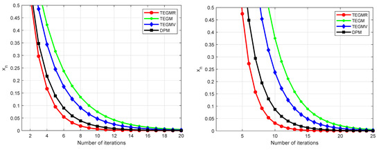
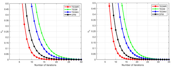
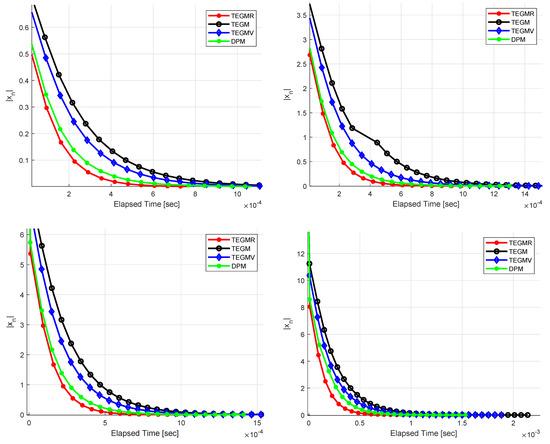
Let $\mathcal{H} = \mathbb{R}$ be the set of real numbers. Define the bifunction $\mathcal{F}(u,v) = uv - u^2$ for all $u,v\in \mathcal{H}$. Let $A:\mathcal{H}\to \mathcal{H}$ be given by $Ax = x$, $f:\mathcal{H}\to \mathcal{H}$ be given by $fx = \frac{2x}{3}$ for all $x\in \mathcal{H}$. We get that A is monotone and 1-Lipschitz continuous. It is easy to check that $T_{{\sigma }_n}^{\mathcal{F}}x = \frac{x}{1 + 2{\sigma }_n}.$ It is also not difficult to check $\mathrm{GEP}(\mathcal{F},\mathcal{A}) = \left\{0\right\}$. Let us choose ${\alpha }_n = \frac{1}{\sqrt{n + 1}}$, ${\sigma }_n = \frac{1}{2}$, $\varsigma = 1$ and $\delta = l = \frac{1}{2}$. We test our Algorithm 3 for different values of $x_0$, see Figure 1, Figure 2 and Figure 3.

Figure 1. Example 1, left: $x_0 = 1$; right: $x_0 = 5$.

Figure 2. Example 1, left: $x_0 = 10$, right: $x_0 = 15$.

Figure 3. Example 1, top left: $x_0 = 1$; top right: $x_0 = 5$, bottom left: $x_0 = 10$, bottom right: $x_0 = 15$.

Example 2.

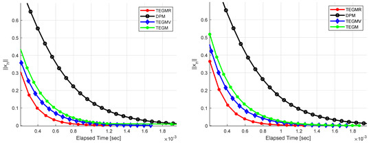
Let $\mathcal{F}:{\mathbb{R}}^m \times {\mathbb{R}}^m\to \mathbb{R}$ be given by $\mathcal{F}(x,y) = xy - x^2$ for all $x,y\in {\mathbb{R}}^m$, $A:{\mathbb{R}}^m\to {\mathbb{R}}^m$ be given by $Ax = x$, $f:{\mathbb{R}}^m\to {\mathbb{R}}^m$ be given by $fx = \frac{2x}{3}$ for all $x\in {\mathbb{R}}^m$. The feasible set C is given by $C = \{x\in {\mathbb{R}}^m:0 \le x_i \le 1,i = 1,\dots ,m\}.$ The maximum number of iterations is 300 as the stopping criterion and the initial values $x_0$ are randomly generated by rand $(0,1)$ in MATLAB. Let us choose ${\alpha }_n = \frac{1}{\sqrt{n + 1}}$, ${\sigma }_n = \frac{1}{2}$, $\varsigma = 1$ and $\delta = l = \frac{1}{2}$. Figure 4 describe the numerical results, for Example 2 in ${\mathbb{R}}^5$ and and ${\mathbb{R}}^{10}$, respectively.

Figure 4. Example 2, Left: $m=5$; Right: $m=10$.

According to all graphical representations in Figure 1, Figure 2, Figure 3 and Figure 4, one finds that Algorithm 3 performs better than than Algorithm (4). Algorithms 1 and 2 in terms of number of iterations and CPU-time taken for computation.

5. Conclusions

This paper presents an alternative regularization method for finding the smallest norm solution of a generalized equilibrium problem. This method can be considered an improvement of the Tseng’s extragradient method and the regularization method. We prove that the iterative process constructed by the proposed method converges strongly to the smallest norm solution of the generalized equilibrium problem. Several numerical experiments are also given to demonstrate the competitive advantage of the suggested methods over other known methods.

References

- Muu, L.D.; Nguyen, V.H.; Quy, N.V. On Nash-Cournot oligopolistic market equilibrium models with concave cost functions. J. Glob. Optim. 2008, 41, 351–364. [Google Scholar] [CrossRef]
- Blum, E.; Oettli, W. From optimization and variational inequalities to equilibrium problems. Math. Stud. 1994, 63, 12–145. [Google Scholar]
- Combettes, P.L.; Hirstoaga, S.A. Equilibrium programming in Hilbert spaces. J. Nonlinear Convex Anal. 2005, 6, 117–136. [Google Scholar]
- Chidume, C.E.; Mărușter, Ș. Iterative methods for the computation of fixed points of demicontractive mappings. J. Comput. Appl. Math. 2010, 234, 861–882. [Google Scholar] [CrossRef]
- Thong, D.V.; Hieu, D.V. Weak and strong convergence theorems for variational inequality problems. Numer. Algorithms 2018, 78, 1045–1060. [Google Scholar] [CrossRef]
- Alakoya, T.; Jolaoso, L.O.; Mewomo, O.T. A general iterative method for finding common fixed point of finite family of demicontractive mappings with accretive variational inequality problems in Banach spaces. Nonlinear Stud. 2020, 27, 213–236. [Google Scholar]
- Ogwo, G.N.; Izuchukwu, C.; Mewomo, O.T. Inertial methods for finding minimum-norm solutions of the split variational inequality problem beyond monotonicity. Numer. Algor. 2021, 88, 1419–1456. [Google Scholar] [CrossRef]
- Cai, G.; Dong, Q.-L.; Peng, Y. Strong convergence theorems for solving variational inequality problems with pseudo-monotone and non-Lipschitz operators. J. Opt. Theory Appl. 2021, 188, 447–472. [Google Scholar] [CrossRef]
- Yao, Y.; Cho, Y.J.; Liou, Y.C. Algorithms of common solutions for variational inclusions, mixed equilibrium problems and fixed point problems. Eur. J. Oper. Res. 2011, 212, 242–250. [Google Scholar] [CrossRef]
- Tan, B.; Qin, X.; Yao, J.C. Strong convergence of self-adaptive inertial algorithms for solving split variational inclusion problems with applications. J. Sci. Comput. 2021, 87, 20. [Google Scholar] [CrossRef]
- Song, Y.L.; Ceng, L.C. Strong convergence of a general iterative algorithm for a finite family of accretive operators in Banach spaces. Fixed Point Theory Appl. 2015, 2015, 90. [Google Scholar] [CrossRef]
- Jolaoso, L.O.; Karahan, I. A general alternative regularization method with line search technique for solving split equilibrium and fixed point problems in Hilbert spaces. Comput. Appl. Math. 2020, 39, 150. [Google Scholar] [CrossRef]
- Korpelevich, G.M. An extragradient method for finding saddle points and for other problems. Matecon 1976, 12, 747–756. [Google Scholar]
- Censor, Y.; Gibali, A.; Reich, S. The subgradient extragradient method for solving variational inequalities in Hilbert space. J. Optim. Theory Appl. 2011, 148, 318–335. [Google Scholar] [CrossRef] [PubMed]
- Tan, B.; Qin, X. Self adaptive viscosity-type inertial extragradient algorithms for solving variational inequalities with applications. Math. Model. Anal. 2022, 27, 41–58. [Google Scholar] [CrossRef]
- Hartman, P.; Stampacchia, G. On some nonlinear elliptic differential functional equations. Acta Math. 1966, 115, 271–310. [Google Scholar] [CrossRef]
- Bnouhachem, A.; Chen, Y. An iterative method for a common solution of generalized mixed equilibrium problem, variational inequalities and hierarchical fixed point problems. Fixed Point Theory Appl. 2014, 2014, 155. [Google Scholar] [CrossRef][Green Version]
- Hieu, D.V.; Quy, P.K.; Duong, H.N. Strong convergence of double-projection method for variational inequality problems. Comput. Appl. Math. 2021, 40, 73. [Google Scholar] [CrossRef]
- Tseng, P. A modified forward-backward splitting method for maximal monotone mappings. SIAM J. Control Optim. 2000, 38, 431–446. [Google Scholar] [CrossRef]
- Dadashi, V.; Iyiola, O.S.; Shehu, Y. The subgradient extragradient method for pseudomonotone equilibrium problems. Optimization 2020, 69, 901–923. [Google Scholar] [CrossRef]
- Rehman, H.U.; Kumam, P.; Dong, Q.L.; Peng, Y.; Deebani, W. A new Popov’s subgradient extragradient method for two classes of equilibrium programming in a real Hilbert space. Optimization 2021, 70, 2675–2710. [Google Scholar] [CrossRef]
- Goebel, K.; Kirk, W.A. Topics in Metric Fixed Point Theory; Cambridge Univ. Press: Cambridge, UK, 1990. [Google Scholar]
- Xu, H.K. Iterative algorithm for nonlinear operators. J. Lond. Math. Soc. 2002, 2, 1–17. [Google Scholar] [CrossRef]
- Xu, H.K. Viscosity approximation methods for nonexpansive mappings. J. Math. Anal. Appl. 2004, 298, 279–291. [Google Scholar] [CrossRef]
Publisher’s Note: MDPI stays neutral with regard to jurisdictional claims in published maps and institutional affiliations. |
© 2022 by the authors. Licensee MDPI, Basel, Switzerland. This article is an open access article distributed under the terms and conditions of the Creative Commons Attribution (CC BY) license (https://creativecommons.org/licenses/by/4.0/).