
The Dynamics between Structural Conditions and Entrepreneurship in Europe: Feature Extraction and System GMM Approaches


Abstract
:1. Introduction
- Question 1—How do the EFCs influence the EI?
- Question 2—How do the EFCs influence the TEA?
2. Data and Methodology
2.1. Data
- EFC1: Financing for entrepreneurs;
- EFC2: Governmental support and policies;
- EFC3: Taxes and bureaucracy;
- EFC4: Governmental programs;
- EFC5: Basic school entrepreneurial education and training;
- EFC6: Post school entrepreneurial education and training;
- EFC7: R & D transfer;
- EFC8: Commercial and professional infrastructure;
- EFC9: Internal market dynamics;
- EFC10: Internal market openness;
- EFC11: Physical and services infrastructure;
- EFC12: Cultural and social norms.
2.2. Methodology
2.2.1. Feature Extraction
Data Adequacy
Retaining Factors
Reliability
2.2.2. System GMM
- Equations in differences:
- Equations in levels:
3. Results
3.1. Feature Extraction—Factor Analysis
3.2. System GMM Results
4. Conclusions and Future Work
Author Contributions
Funding
Institutional Review Board Statement
Informed Consent Statement
Data Availability Statement
Conflicts of Interest
References
- Farinha, L.; Lopes, J.; Bagchi-Sen, S.; Sebastião, J.R.; Oliveira, J. Entrepreneurial dynamics and government policies to boost entrepreneurship performance. Socio-Econ. Plan. Sci. 2020, 72, 100950. [Google Scholar] [CrossRef]
- Fernandes, A.J.; Ferreira, J.J. Entrepreneurial ecosystems and networks: A literature review and research agenda. Rev. Manag. Sci. 2022, 16, 189–247. [Google Scholar] [CrossRef]
- Hong, S.; Robert Reed, W.; Tian, B.; Wu, T.; Chen, G. Does FDI promote entrepreneurial activities? A meta-analysis. World Dev. 2021, 142, 105436. [Google Scholar] [CrossRef]
- Thompson, E.R. Individual entrepreneurial intent: Construct clarification and development of an internationally reliable metric. Entrep. Theory Pract. 2009, 33, 669–694. [Google Scholar] [CrossRef]
- Valliere, D. Reconceptualizing entrepreneurial framework conditions. Int. Entrep. Manag. J. 2010, 6, 97–112. [Google Scholar] [CrossRef]
- Orobia, L.A.; Tusiime, I.; Mwesigwa, R.; Ssekiziyivu, B. Entrepreneurial framework conditions and business sustainability among the youth and women entrepreneurs. Asia Pac. J. Innov. Entrep. 2020, 14, 60–75. [Google Scholar] [CrossRef]
- Global Entrepreneurship Research Association. Global Entrepreneurship Monitor; 2016/17 Global Report; Global Entrepreneurship Research Association: London, UK, 2017. [Google Scholar]
- Kelley, D.; Bosma, N.; Amorós, J.E. Global Entrepreneurship Monitor; 2010 Executive Report; Global Entrepreneurship Research Association: London, UK, 2011. [Google Scholar]
- Bergmann, H.; Mueller, S.; Schrettle, T. The use of global entrepreneurship monitor data in academic research: A critical inventory and future potentials. Int. J. Entrep. Ventur. 2014, 6, 242–276. [Google Scholar] [CrossRef]
- Costa e Silva, E.; Correia, A.; Duarte, F. How Portuguese experts’ perceptions on the entrepreneurial framework conditions have changed over the years: A benchmarking analysis. AIP Conf. Proc. 2018, 2040, 110005. [Google Scholar]
- Sampaio, C.; Correia, A.; Braga, V.; Braga, A. Environmental variables and entrepreneurship—A study with GEM NES global individual level data. Int. J. Knowl. Based Dev. 2016, 2040, 4476. [Google Scholar]
- Costa e Silva, E.; Correia, A.; Borges, A. Unveiling the dynamics of the European entrepreneurial framework conditions over the last two decades: A cluster analysis. Axioms 2021, 10, 149. [Google Scholar] [CrossRef]
- Braga, V.; Queirós, M.; Correia, A.; Braga, A. High-growth business creation and management: A multivariate quantitative approach using GEM data. J. Knowl. Econ. 2018, 9, 424–445. [Google Scholar] [CrossRef]
- Pilar, M.D.F.; Marques, M.; Correia, A. New and growing firms’ entrepreneurs’ perceptions and their discriminant power in EDL countries. Glob. Bus. Econ. Rev. 2019, 21, 474–499. [Google Scholar] [CrossRef]
- Levie, J.; Autio, E. Entrepreneurial framework conditions and national-level entrepreneurial activity: Seven-year panel study. In Proceedings of the Third Global Entrepreneurship Research Conference, San Francisco, CA, USA, 28–31 March 2007; pp. 1–39. [Google Scholar]
- Van Stel, A.; Carree, M.; Thurik, R. The effect of entrepreneurial activity on national economic growth. Small Bus. Econ. 2005, 24, 311–321. [Google Scholar] [CrossRef] [Green Version]
- Roodman, D. How to do xtabond2: An introduction to difference and system GMM in Stata. Stata J. 2009, 9, 86–136. [Google Scholar] [CrossRef] [Green Version]
- Jolliffe, I.T.; Cadima, J. Principal component analysis: A review and recent developments. Philos. Trans. R. Soc. A: Math. Phys. Eng. Sci. 2016, 374, 20150202. [Google Scholar] [CrossRef]
- Jolliffe, I. Principal component analysis. In Encyclopedia of Statistics in Behavioral Science; John Wiley & Sons, Ltd.: Hoboken, NJ, USA, 2005. [Google Scholar]
- Sarmento, R.; Costa, V. Comparative Approaches to Using R and Python for Statistical Data Analysis; IGI Global: Hershey, PA, USA, 2017. [Google Scholar]
- Cureton, E.E.; D’Agostino, R.B. Factor Analysis: An Applied Approach; Psychology Press: East Sussex, UK, 2013. [Google Scholar]
- Cangelosi, R.; Goriely, A. Component retention in principal component analysis with application to cDNA microarray data. Biol. Direct 2007, 2, 1–21. [Google Scholar] [CrossRef] [Green Version]
- Cronbach, L.J. Coefficient alpha and the internal structure of tests. Psychometrika 1951, 16, 297–334. [Google Scholar] [CrossRef] [Green Version]
- Tavakol, M.; Dennick, R. Making sense of Cronbach’s alpha. Int. J. Med. Educ. 2011, 2, 53. [Google Scholar] [CrossRef]
- Bound, J.; Jaeger, D.A.; Baker, R.M. Problems with instrumental variables estimation when the correlation between the instruments and the endogenous explanatory variable is weak. J. Am. Stat. Assoc. 1995, 90, 443–450. [Google Scholar] [CrossRef]
- Mohammadi Khyareh, M.; Rostami, N. The Impact of Macroeconomic Variables on Entrepreneurship: Generalized Method of Moments (GMM). J. Macroecon. 2021, 15, 30–55. [Google Scholar]
- Jafari-Sadeghi, V.; Sukumar, A.; Pagán-Castaño, E.; Dana, L.P. What drives women towards domestic vs international business venturing? An empirical analysis in emerging markets. J. Bus. Res. 2021, 134, 647–660. [Google Scholar] [CrossRef]
- Afawubo, K.; Noglo, Y.A. ICT and entrepreneurship: A comparative analysis of developing, emerging and developed countries. Technol. Forecast. Soc. Change 2022, 175, 121312. [Google Scholar] [CrossRef]
- Dutta, N.; Sobel, R.S. Entrepreneurship, fear of failure, and economic policy. Eur. J. Political Econ. 2021, 66, 101954. [Google Scholar] [CrossRef]
- Nickell, S. Biases in dynamic models with fixed effects. Econom. J. Econom. Soc. 1981, 6, 1417–1426. [Google Scholar] [CrossRef]
- Anderson, T.W.; Hsiao, C. Formulation and estimation of dynamic models using panel data. J. Econom. 1982, 18, 47–82. [Google Scholar] [CrossRef]
- Arellano, M.; Bover, O. Another look at the instrumental variable estimation of error-components models. J. Econom. 1995, 68, 29–51. [Google Scholar] [CrossRef] [Green Version]
- Blundell, R.; Bond, S. Initial conditions and moment restrictions in dynamic panel data models. J. Econom. 1998, 87, 115–143. [Google Scholar] [CrossRef] [Green Version]
- Wooldridge, J.M. Introductory Econometrics: A Modern Approach; Cengage Learning: Boston, MA, USA, 2015. [Google Scholar]
- Albulescu, C.T.; Tămăşilă, M. Exploring the role of FDI in enhancing the entrepreneurial activity in Europe: A panel data analysis. Int. Entrep. Manag. J. 2016, 12, 629–657. [Google Scholar] [CrossRef]
- Acs, Z.J.; Desai, S.; Hessels, J. Entrepreneurship, economic development and institutions. Small Bus. Econ. 2008, 31, 219–234. [Google Scholar] [CrossRef] [Green Version]
- Van Stel, A.; Storey, D.J.; Thurik, A.R. The effect of business regulations on nascent and young business entrepreneurship. Small Bus. Econ. 2007, 28, 171–186. [Google Scholar] [CrossRef] [Green Version]
- Hechavarría, D.M.; Ingram, A.E. Entrepreneurial ecosystem conditions and gendered national-level entrepreneurial activity: A 14-year panel study of GEM. Small Bus. Econ. 2019, 53, 431–458. [Google Scholar] [CrossRef]

| Country | # | Country | # |
|---|---|---|---|
| Spain | 19 | Poland, Portugal | 10 |
| Croatia, Germany, Ireland, Slovenia | 18 | Slovakia | 9 |
| United Kingdom, Greece | 17 | Bosnia and Herzegovina, Iceland | 8 |
| Finland, Italy, Netherlands, Norway | 16 | Luxemburg, North Macedonia | 7 |
| Switzerland | 15 | Austria, Estonia | 6 |
| Hungary, Sweden | 13 | Romania | 5 |
| Belgium, Russia | 12 | Cyprus, Bulgaria, Lithuania | 4 |
| Denmark, France, Latvia | 11 | Czech Republic, Serbia | 3 |
| Rotated | |||||
|---|---|---|---|---|---|
| Component Matrix | Communalities | ||||
| EFC | Description | MSA | F1 | F2 | |
| 4 | Governmental programs | 0.914 | 0.774 | 0.730 | |
| 7 | R&D transfer | 0.919 | 0.738 | 0.765 | |
| 9 | Internal market dynamics | 0.750 | −0.718 | 0.576 | |
| 2 | Governmental support and policies | 0.915 | 0.700 | 0.670 | |
| 8 | Commercial and professional infrastructure | 0.902 | 0.698 | 0.653 | |
| 10 | Internal market openness | 0.928 | 0.650 | 0.690 | |
| 1 | Financing for entrepreneurs | 0.911 | 0.626 | 0.495 | |
| 11 | Physical and services infrastructure | 0.891 | 0.608 | 0.437 | |
| 12 | Cultural and social norms | 0.839 | 0.860 | 0.779 | |
| 5 | Basic school entrepreneurial education and training | 0.893 | 0.784 | 0.630 | |
| 6 | Post school entrepreneurial education and training | 0.905 | 0.653 | 0.514 | |
| 3 | Taxes and bureaucracy | 0.905 | 0.639 | 0.689 | |
| % of variance | 35.367 | 28.206 | 63.573 | ||
| Cronbach’s alpha | 0.810 | 0.782 | KMO | ||
| Number of items | 8 | 4 | 0.898 | ||
| EFC | 02 | 03 | 04 | 05 | 06 | 07 | 08 | 09 | 10 | 11 | 12 | 13 | 14 | 15 | 16 | 17 | 18 | 19 | # |
|---|---|---|---|---|---|---|---|---|---|---|---|---|---|---|---|---|---|---|---|
| 1 | F1 | F1 | F1 | F1 | F1 | F1 | F1 | F1 | F1 | F1 | F1 | F1 | F1 | F1 | F1 | F1 | F1 | F1 | 18 |
| 2 | F1 | F1 | F1 | F1 | F1 | F1 | F1 | F1 | F1 | F1 | F1 | F1 | F1 | F1 | 14 | ||||
| 3 | F1 | F1 | F1 | F1 | F1 | F1 | F1 | F1 | 8 | ||||||||||
| 4 | F1 | F1 | F1 | F1 | F1 | F1 | F1 | F1 | F1 | F1 | F1 | F1 | F1 | F1 | F1 | 15 | |||
| 5 | F1 | F1 | F1 | F1 | F1 | F1 | F1 | F1 | 8 | ||||||||||
| 6 | F1 | F1 | F1 | F1 | F1 | F1 | F1 | F1 | F1 | 9 | |||||||||
| 7 | F1 | F1 | F1 | F1 | F1 | F1 | F1 | F1 | F1 | F1 | F1 | F1 | F1 | F1 | F1 | F1 | 16 | ||
| 8 | F1 | F1 | F1 | F1 | F1 | F1 | F1 | F1 | F1 | F1 | F1 | F1 | 12 | ||||||
| 9 | F1 | F1 | F1 | F1 | F1 | F1 | F1 | F1 | F1 | 9 | |||||||||
| 10 | F1 | F1 | F1 | F1 | F1 | F1 | F1 | F1 | F1 | F1 | F1 | F1 | F1 | 13 | |||||
| 11 | F1 | F1 | F1 | F1 | F1 | F1 | F1 | F1 | F1 | F1 | F1 | F1 | F1 | 13 | |||||
| 12 | F1 | F1 | F1 | F1 | F1 | F1 | F1 | F1 | 8 |
| Year | KMO | Total | # of | TVE | MSA < 0.4 | Com. < 0.5 | |
|---|---|---|---|---|---|---|---|
| TVE | Factors | 3 Factors | 2 Factors | ||||
| 2002 | 0.52 | 81% | 4 | 72% | 58% | 5, 6, 11, 12 | 6 |
| 2003 | 0.56 | 77% | 4 | 68% | 54% | 5 | – |
| 2004 | 0.49 | 71% | 3 | 71% | 60% | 5, 12, 11 | 1, 11 |
| 2005 | 0.50 | 76% | 3 | 76% | 64% | 6 | – |
| 2006 | 0.71 | 76% | 3 | 76% | 64% | 6 | |
| 2007 | 0.64 | 81% | 4 | 76% | 65% | 6 | |
| 2008 | 0.63 | 76% | 3 | 76% | 73% | 6 | – |
| 2009 | 0.68 | 75% | 2 | 81% | 75% | 6 | – |
| 2010 | 0.57 | 75% | 3 | 75% | 65% | 9, 6 | – |
| 2011 | 0.63 | 80% | 3 | 80% | 69% | 9 | – |
| 2012 | 0.84 | 80% | 3 | 80% | 71% | – | – |
| 2013 | 0.86 | 70% | 2 | 77% | 70% | – | – |
| 2014 | 0.84 | 76% | 3 | 76% | 67% | – | – |
| 2015 | 0.75 | 80% | 3 | 80% | 70% | 9 | – |
| 2016 | 0.80 | 68% | 2 | 75% | 68% | – | – |
| 2017 | 0.77 | 74% | 2 | 81% | 74% | – | – |
| 2018 | 0.68 | 75% | 3 | 75% | 65% | 9 | – |
| 2019 | 0.82 | 74% | 2 | 81% | 74% | – | – |
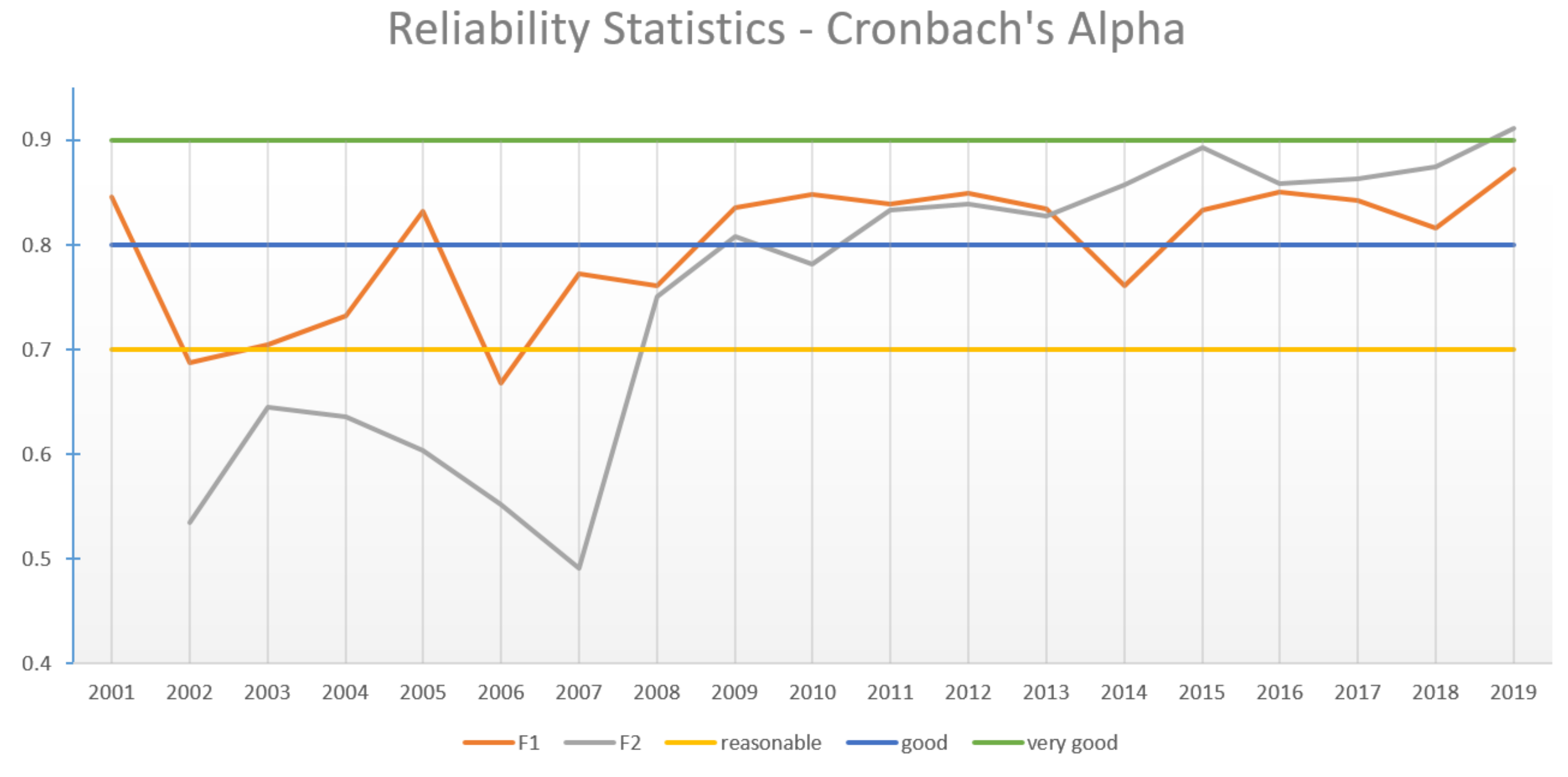
| Year | F1 | F2 | # Countries | Year | F1 | F2 | # Countries |
|---|---|---|---|---|---|---|---|
| 2000 | 0.748 | * | 11 | 2010 | 0.848 | 0.782 | 21 |
| 2001 | 0.846 | ** | 14 | 2011 | 0.839 | 0.833 | 22 |
| 2002 | 0.687 | 0.535 | 16 | 2012 | 0.849 | 0.839 | 28 |
| 2003 | 0.705 | 0.645 | 17 | 2013 | 0.834 | 0.827 | 28 |
| 2004 | 0.732 | 0.636 | 15 | 2014 | 0.761 | 0.858 | 29 |
| 2005 | 0.832 | 0.604 | 18 | 2015 | 0.833 | 0.893 | 24 |
| 2006 | 0.668 | 0.552 | 18 | 2016 | 0.851 | 0.859 | 25 |
| 2007 | 0.772 | 0.491 | 17 | 2017 | 0.842 | 0.863 | 20 |
| 2008 | 0.761 | 0.75 | 14 | 2018 | 0.816 | 0.875 | 20 |
| 2009 | 0.836 | 0.808 | 19 | 2019 | 0.872 | 0.911 | 22 |
| Variables | Dependent Variable EI | Dependent Variable TEA | ||||
|---|---|---|---|---|---|---|
| Full Sample | 2001–2008 | 2009–2019 | Full Sample | 2001–2008 | 2009–2019 | |
| EI/TEA | 0.785 *** | 0.714 *** | 0.760 *** | 0.632 *** | 0.487 *** | 0.582 *** |
| (0.038) | (0.049) | (0.053) | (0.061) | (0.140) | (0.085) | |
| EFC1 | −1.000 | −1.121 | −0.973 | −0.171 | −0.138 | 0.126 |
| (0.754) | (1.038) | (0.970) | (0.407) | (0.695) | (0.515) | |
| EFC2 | 0.170 | −1.766 ** | 0.873 | −0.315 | −1.129 | −0.305 |
| (0.484) | (0.789) | (0.606) | (0.288) | (0.698) | (0.329) | |
| EFC3 | 0.495 | 0.520 | 0.350 | 0.118 | 1.100 * | −0.331 |
| (0.481) | (0.633) | (0.611) | (0.292) | (0.564) | (0.332) | |
| EFC4 | 0.373 | 0.244 | 0.899 | 0.605 | 0.763 | 0.677 * |
| (0.469) | (0.938) | (0.791) | (0.359) | (0.819) | (0.396) | |
| EFC5 | −0.206 | −1.098 | 0.379 | 0.255 | −0.071 | 0.237 |
| (0.499) | (1.255) | (0.809) | (0.294) | (0.813) | (0.423) | |
| EFC6 | 0.936 | 0.292 | 1.114 | 0.539 | 0.093 | 1.035 * |
| (0.625) | (0.783) | (1.156) | (0.343) | (0.950) | (0.526) | |
| EFC7 | −0.367 | 1.108 | −0.895 | −1.724 *** | −0.374 | −2.631 *** |
| (0.816) | (2.358) | (1.159) | (0.600) | (1.301) | (0.709) | |
| EFC8 | 1.337 * | 3.454 * | 1.327 | 0.107 | −0.789 | 0.430 |
| (0.665) | (1.815) | (0.827) | (0.442) | (1.121) | (0.492) | |
| EFC9 | 0.632 | 0.965 | 0.463 | −0.209 | -0.111 | −0.244 |
| (0.472) | (0.833) | (0.586) | (0.205) | (0.491) | (0.254) | |
| EFC10 | −0.079 | 0.202 | −0.786 | 0.448 | −0.253 | 0.744 |
| (0.715) | (1.193) | (0.980) | (0.473) | (1.010) | (0.566) | |
| EFC11 | −0.288 | 0.317 | −0.969 * | 0.233 | 0.154 | −0.019 |
| (0.323) | (0.647) | (0.520) | (0.234) | (0.485) | (0.300) | |
| EFC12 | −0.479 | 0.427 | −0.560 | 0.909 * | 0.855 | 1.227 * |
| (0.549) | (1.094) | (0.763) | (0.453) | (0.878) | (0.611) | |
| Control | ||||||
| GDP_pc | −0.000 *** | −0.000 ** | −0.000 *** | −0.000 | −0.000 | −0.000 |
| Instrumental | (0.000) | (0.000) | (0.000) | (0.000) | (0.000) | (0.000) |
| Population_total | −0.000 *** | −0.000 *** | −0.000 *** | −0.000 *** | −0.000 *** | −0.000 *** |
| (0.000) | (0.000) | (0.000) | (0.000) | (0.000) | (0.000) | |
| Year dummies | yes | yes | yes | yes | yes | yes |
| F statistic | 533.37 *** | 3083.76 *** | 533.37 *** | 650.91 *** | 13624.15 *** | 1428.25 *** |
| Hansen test statistic | 0.98 | 0.98 | 0.98 | 3.0 | 3.0 | 3.40 |
| Arellano–Bond statistic | ||||||
| AR(1) | −3.48 *** | −2.94 *** | −3.48 *** | −3.58 *** | −2.90 *** | −3.33 *** |
| AR(2) | 1.34 | 0.49 | 1.34 | 0.36 | −0.79 | 0.77 |
Publisher’s Note: MDPI stays neutral with regard to jurisdictional claims in published maps and institutional affiliations. |
© 2022 by the authors. Licensee MDPI, Basel, Switzerland. This article is an open access article distributed under the terms and conditions of the Creative Commons Attribution (CC BY) license (https://creativecommons.org/licenses/by/4.0/).
Share and Cite
Borges, A.; Correia, A.; Costa e Silva, E.; Carvalho, G. The Dynamics between Structural Conditions and Entrepreneurship in Europe: Feature Extraction and System GMM Approaches. Mathematics 2022, 10, 1349. https://doi.org/10.3390/math10081349
Borges A, Correia A, Costa e Silva E, Carvalho G. The Dynamics between Structural Conditions and Entrepreneurship in Europe: Feature Extraction and System GMM Approaches. Mathematics. 2022; 10(8):1349. https://doi.org/10.3390/math10081349
Chicago/Turabian StyleBorges, Ana, Aldina Correia, Eliana Costa e Silva, and Glória Carvalho. 2022. "The Dynamics between Structural Conditions and Entrepreneurship in Europe: Feature Extraction and System GMM Approaches" Mathematics 10, no. 8: 1349. https://doi.org/10.3390/math10081349
APA StyleBorges, A., Correia, A., Costa e Silva, E., & Carvalho, G. (2022). The Dynamics between Structural Conditions and Entrepreneurship in Europe: Feature Extraction and System GMM Approaches. Mathematics, 10(8), 1349. https://doi.org/10.3390/math10081349