Sliding Mode Controller Based on the Extended State Observer for Plant-Protection Quadrotor Unmanned Aerial Vehicles

Abstract

Owing to the complex dynamics of quadrotor unmanned aerial vehicles (UAVs) and their susceptibility to unknown interferences in an actual working environment, the flight control accuracy of UAVs is extremely high. Moreover, their anti-interference ability is particularly important. This study designed a sliding-mode controller based on the extended state observer. The position control was obtained through the outer-loop position controller. The attitude control was determined through the inner-loop attitude controller. The input of the UAV system was obtained through the controller. The boundary-layer function was used to weaken the oscillatory response of the system, and the traditional extended state observer was improved to improve the response speed, robustness, and tracking accuracy of the controller. For the entire process, the input and output state information of the system and total internal and external disturbances were estimated in real-time through the extended state observer. A sliding-mode control law was designed to compensate for the estimated disturbance in real-time to realize attitude control. Finally, Lyapunov theory was used to confirm the stability of the system. The simulation results demonstrated the improved anti-interference and tracking ability of the designed controller.

1. Introduction

Quadrotor unmanned aerial vehicles (UAVs) are efficient, flexible, small, and convenient, which paved the way for their usage in agricultural and military fields and, consequently, their promising and unlimited application prospects [1]. A quadrotor UAV is a representative of a nonlinear system with strong coupling. It is a complex underactuated system with four control inputs and a six-degrees-of-freedom output. Moreover, quadrotor UAVs can achieve six-degrees-of-freedom flight and average anti-interference ability. However, their aerodynamic characteristics are easily disturbed by the external environment. For UAVs used in plant protection, which carry pesticides for spraying, their control method is important as they operate mostly in an outdoor environment [2].

At present, researchers have proposed several control methods [3]. The traditional proportional-integral-derivative (PID) control algorithm is a simple approach; however, with this algorithm, it is difficult to self-adjust the control parameters with environmental changes [4]. Badr et al. [5] designed a PID controller for a quadrotor UAV, which achieved weak anti-interference ability. Yobi and Shuxi [6] proposed a hover control for a PID quadrotor UAV based on fuzzy self-tuning. However, the mathematical model of the backstepping control (BSC) has high requirements. Unknown interference results in the insufficient accuracy of the model, which often affects the tracking effect of the system. Zuo and Mallikarjunan [7] and Djamel et al. [8] proposed a control method for rotorcraft based on BSC whereby its control effect was improved compared with the traditional PID control. Yin et al. [9] proposed a backstepping method for a quadrotor UAV, which demonstrated good robustness; however, it was deemed unsuitable for different trajectories. An adaptive backstepping fast terminal sliding-mode controller (SMC) for a quadrotor UAV was proposed by Labbadi and Cherkaoui [10]. Zhang et al. [11] combined backstepping and a state observer to eliminate disturbances. For rotorcrafts subject to uncertain effects, such as non-modeling dynamics and external disturbances, Chen et al. [12] and Jeong and Chwa [13] used a control method based on sliding mode, whereas Shao et al. [14] used a control method based on the sliding-mode dynamic surface. These methods are designed under the condition of a known upper bound of uncertainty. However, the actual operation of plant-protection UAVs is usually unknown.

Han, J.Q. [15] proposed active disturbance rejection control, a new control technology that does not depend on an accurate system model. Cheng, Y et al. [16] applied ADRC to the distillation column process and achieved good results. Zheng and Gao [17] developed a linear ADRC method and introduced the concept of “frequency scale”. To clearly define the parameters, the workload of parameter tuning was greatly reduced to facilitate practical applications. Yun-jie et al. [18] introduced variable structure control theory into the extended state observer (ESO) of the ADRC, which ensured the control effect of the original controller and decreased the adjustable parameters. Da-yu et al. [19] and Xing-ling and Hong-lun [20] obtained more system-state information by improving the ESO, thereby improving the observation accuracy of the “total disturbance.” Liu et al. [21] reconstructed the ESO and nonlinear error-feedback controller to avoid high-frequency chattering caused by non-smooth functions in traditional ADRC. Zhang et al. [22] used ADRC to verify the anti-interference ability of the quadrotor UAV, which obtained a good trajectory-tracking effect.

In this study, a control method with better robustness, tracking accuracy, and responsiveness was selected from SMC and BSC to improve the ability of plant-protection UAVs to complete work tasks in complex environments by designing a controller in a disturbance-free environment. The designed controller combined this control method with an improved ESO to realize a real-time estimation and compensation of complex disturbances. The effectiveness of the ESO and controller was verified by stability analysis. The performance of the algorithm was demonstrated by simulations.

2. Quadrotor UAV Dynamics Model

As quadrotor UAVs are typically underactuated systems, they are simplified for analysis in modeling, and the following four assumptions were made: (1) a quadrotor UAV has a uniformly symmetrical rigid body exhibiting no change in mass or rotational inertia during flight; (2) the center of mass of a quadrotor UAV coincides with the geometric center of its airframe; (3) the resistance and gravity of a quadrotor UAV are not affected by factors such as flight height and remain unchanged; (4) and air resistance and gyroscopic effects are ignored.

2.1. Establishing the Coordinate System

Li J et al. [23] built a mathematical model of a quadrotor UAV. Figure 1 shows a diagram of the movement of the quadrotor UAV. To describe the model of the quadrotor UAV, the earth coordinate system $E-x_e, y_e, z_e$ and body coordinate system $B-x_b, y_b, z_b$ of the quadrotor should be established first. The conversion relationship from the earth coordinate system to the body coordinate system is shown in Equation (1).

$$\begin{array}{c}R=\left(\begin{array}{ccc}\cos \psi \cos \theta & \sin \varphi \sin \theta \cos \psi -\cos \varphi \sin \psi & \cos \varphi \sin \theta \cos \psi +\sin \varphi \sin \psi \\ \cos \theta \sin \psi & \sin \varphi \sin \theta \sin \psi +\cos \varphi \cos \psi & \cos \varphi \sin \theta \sin \psi -\sin \varphi \cos \psi \\ -\sin \theta & \sin \varphi \cos \theta & \cos \varphi \cos \theta \end{array}\right)\end{array}$$

(1)

2.2. Quadrotor Dynamic Modeling

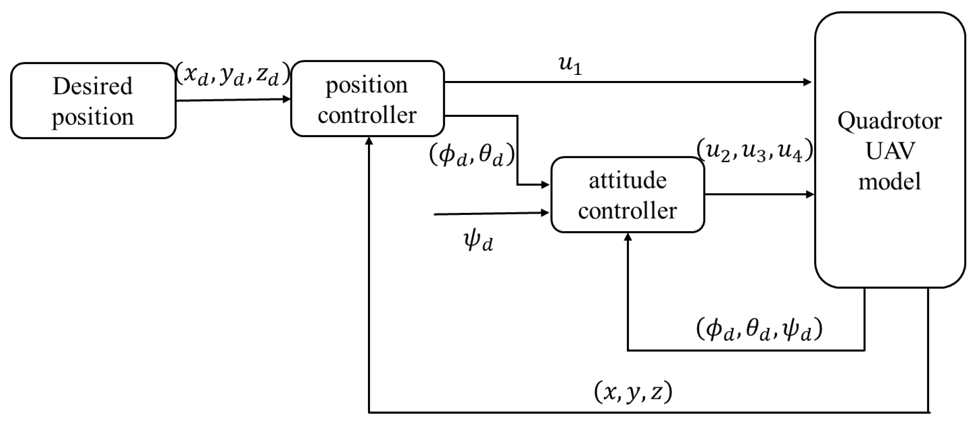
Neglecting the air resistance during flight and after analyzing the force of the UAV, the dynamic model of the quadrotor UAV can be further obtained, and the position and attitude controls can be obtained using Equations (2) and (3), respectively, as follows:

$$\begin{array}{c}\left\{\begin{array}{c}\ddot{x}=\frac{b\left({\omega }_1^2+{\omega }_2^2+{\omega }_3^2+{\omega }_4^2\right)}{m}\left(\cos \varphi \sin \theta \cos \psi +\sin \varphi \sin \psi \right)\\ \ddot{y}=\frac{b\left({\omega }_1^2+{\omega }_2^2+{\omega }_3^2+{\omega }_4^2\right)}{m}\left(\cos \varphi \sin \theta \sin \psi -\sin \varphi \cos \psi \right)\\ \ddot{z}=\frac{b\left({\omega }_1^2+{\omega }_2^2+{\omega }_3^2+{\omega }_4^2\right)}{m}\left(\cos \varphi \cos \theta \right)-g \end{array}\right.\end{array}$$

(2)

$$\begin{array}{c}\left\{\begin{array}{c}\ddot{\varphi }=\frac{I_y-I_z}{I_x}\dot{\theta }\dot{\psi }+\frac{bl\left({\omega }_4^2-{\omega }_2^2\right)}{I_x} \\ \ddot{\theta }=\frac{I_z-I_x}{I_y}\dot{\varphi }\dot{\psi }+\frac{bl\left({\omega }_3^2-{\omega }_1^2\right)}{I_x} \\ \ddot{\psi }=\frac{I_x-I_y}{I_z}\dot{\varphi }\dot{\theta }+\frac{d\left({\omega }_1^2+{\omega }_3^2-{\omega }_2^2-{\omega }_4^2\right)}{I_z}\end{array}\right.\end{array}$$

(3)

where $b$ is the lift coefficient; $d$ is the drag coefficient; $l$ is the distance from the rotor to the center of the body; ${\omega }_n\left(n=1, 2, 3, 4\right)$ is the rotation speed of each rotor; and $I_x$, $I_y$, and $I_z$ are the moments of inertia on the $x$, $y$, and $z$ axes, respectively.

3. SMC Design

The SMC design is determined as follows:

$$\begin{array}{c}\left\{\begin{array}{c}\begin{array}{c}{u}_1=b\left({\omega }_1^2+{\omega }_2^2+{\omega }_3^2+{\omega }_4^2\right)\\ u_2=b\left({\omega }_4^2-{\omega }_2^2\right) \end{array}\\ \begin{array}{c}{u}_3=b\left({\omega }_3^2-{\omega }_1^2\right) \\ u_4=d\left({\omega }_1^2+{\omega }_3^2-{\omega }_2^2-{\omega }_4^2\right)\end{array}\end{array}\right.\end{array}$$

(4)

As the UAV system is in a strongly coupled state, it is difficult to solve it using a single-stage controller. Thus, a cascade controller, as shown in Figure 2, was used.

3.1. Design of the Position SMC

The controlled quantities and feedback input of the controller were labeled as $x$,$y$, and $z$. Taking the height control $z$ as an example, a sliding-mode position controller was designed because the position controller is affected by the attitude controller, which was designed as the outer loop.

First, with the state variable defined as $P=\left[x \dot{x} y \dot{y} z \dot{z} \varphi \dot{\varphi } \theta \dot{\theta } \psi \dot{\psi }\right]$, a disturbance-free altitude controller was designed using the position state in Equation (2):

$$\begin{array}{c}\left\{\begin{array}{c}{\dot{p}}_1=p_2=\dot{z} \\ {\dot{p}}_2=\ddot{z}=\frac{u_1}{m}\cos \varphi \cos \theta -g\end{array}\right.\end{array}$$

(5)

Setting the desired height as $z_d$, the height error and its derivative can be defined as:

$$\begin{array}{c}{e}_z=z_d-z\end{array}$$

(6)

$$\begin{array}{c}{\dot{e}}_z={\dot{z}}_d-\dot{z}\end{array}$$

(7)

The sliding surface is designed as:

$$\begin{array}{c}{S}_z=\dot{z}-{\dot{z}}_d-{\alpha }_z{e}_z\end{array}$$

(8)

where ${\alpha }_z>0$.

According to the second method of Lyapunov, if the scalar function $V_{\left(x\right)}$ satisfies:

(1)

$V_{\left(x\right)}=0$ if and only if $x=0$;

(2)

$V_{\left(x\right)}>0$ if and only if $x\ne 0$;

(3)

${\dot{V}}_{\left(x\right)}\le 0$ when $x\ne 0$;

Then the system is stable. In particular, if $x\ne 0$, ${\dot{V}}_{\left(x\right)}<0$, then the system is asymptotically stable.

The Lyapunov function is defined as:

$$\begin{array}{c}{V}_1=\frac{1}{2}{S}_Z^2\end{array}$$

(9)

$$\begin{array}{c}{\dot{V}}_1=S_Z{\dot{S}}_Z=S_Z\left(\frac{u_1}{m}\cos \varphi \cos \theta -g-{\ddot{z}}_d-{\alpha }_z{\dot{e}}_z\right)\end{array}$$

(10)

Using the exponential approach law, we obtain:

$$\begin{array}{c}\dot{S}=-\epsilon sign\left(S\right)-\rho S \epsilon >0, \rho >0\end{array}$$

(11)

Subsequently, the SMC based on the exponential reaching law can be solved as:

$$\begin{array}{c}{u}_1=\frac{m}{\cos \varphi \cos \theta }\left(-{\epsilon }_{z}sign\left(S_z\right)-{\rho }_z{S}_z+{\ddot{z}}_d+{\alpha }_z{\dot{e}}_z+g\right)\end{array}$$

(12)

where ${\epsilon }_z>0$, ${\rho }_z>0$. Substituting Equation (12) for Equation (10), we obtain:

$$\begin{array}{c}{\dot{V}}_1=S_z\left(-{\epsilon }_{z}sign\left(S_z\right)-{\rho }_z{S}_z\right)=-{\epsilon }_z\left|S_z\right|-{\rho }_z{S}_z^2\le 0\end{array}$$

(13)

Thus, the Lyapunov stability condition is satisfied.

Similarly, the two controllers for the x and y channels were designed. From Equation (2), the $x$ and $y$ state equations can be respectively obtained as:

$$\begin{array}{c}\left\{\begin{array}{c}{\dot{p}}_3=p_4=\dot{x} \\ {\dot{p}}_4=\ddot{x}=\frac{u_1}{m}{u}_x\end{array}\right.\end{array}$$

(14)

$$\begin{array}{c}\left\{\begin{array}{c}{\dot{p}}_5=p_6=\dot{y } \\ {\dot{p}}_6=\ddot{y}=\frac{u_1}{m}{u}_y\end{array}\right.\end{array}$$

(15)

$$\begin{array}{c}\left\{\begin{array}{c}{u}_x=\cos \varphi \sin \theta \cos \psi +\sin \varphi \sin \psi \\ u_y=\cos \varphi \sin \theta \sin \psi -\sin \varphi \cos \psi \end{array}\right.\end{array}$$

(16)

The control quantities of $x$ and $y$ can be obtained as:

$$\begin{array}{c}{u}_x=\frac{m}{u_1}\left(-{\epsilon }_{x}sign\left(S_x\right)-{\rho }_x{S}_x+{\ddot{x}}_d+{\alpha }_x{\dot{e}}_x\right) u_1\ne 0\end{array}$$

(17)

where ${\epsilon }_x>0$, ${\rho }_x>0$, $e_x=x_d-x$, ${\dot{e}}_x={\dot{x}}_d-\dot{x}$, $S_x=\dot{x}-{\dot{x}}_d-{\alpha }_x{e}_x$, ${\alpha }_y>0$. If $u_1=0$, $u_x=0$.

$$\begin{array}{c}{u}_y=\frac{m}{u_1}\left(-{\epsilon }_{y}sign\left(S_y\right)-{\rho }_y{S}_y+{\ddot{y}}_d+{\alpha }_y{\dot{e}}_y\right) u_1\ne 0\end{array}$$

(18)

where ${\epsilon }_y>0$, ${\rho }_y>0$, $e_y=y_d-y$, ${\dot{e}}_y={\dot{y}}_d-\dot{y}$, $S_y=\dot{y}-{\dot{y}}_d-{\alpha }_y{e}_y$, ${\alpha }_y>0$. If $u_1=0$, $u_y=0$.

Subsequently, the desired angle ${\varphi }_d$ can be obtained by the inverse solution, and ${\theta }_d$ is obtained as:

$$\begin{array}{c}{\varphi }_d={\sin }^{-1}\left(u_x\sin \psi -u_y\cos \psi \right)\end{array}$$

(19)

$$\begin{array}{c}{\theta }_d={\sin }^{-1}\left(\left(u_x-\sin \varphi \sin \psi \right)/\left(\cos \varphi \cos \psi \right)\right)\end{array}$$

(20)

3.2. Design of the Attitude SMC

As attitude is not affected by position, the attitude control was designed as an inner loop. The expected angles ${\varphi }_d$ and ${\theta }_d$ obtained from the inverse solution of the position controller and set ${\psi }_d$ were used as the input of the attitude controller. Taking the roll angle ϕ as an example, the attitude SMC was designed.

From Equation (3), the state equation of the ϕ channel can be obtained as:

$$\begin{array}{c}\left\{\begin{array}{c}{\dot{p}}_7=p_8=\dot{\varphi } \\ {\dot{p}}_8=\ddot{\varphi }=a_1{\dot{\theta }}_d{\dot{\psi }}_d+b_1{u}_2\end{array}\right.\end{array}$$

(21)

where $a_1=\left(I_y-I_z\right)/I_x$, $b_1=l/I_x$.

The expected angle ${\varphi }_d$ and the error and its derivative are defined as:

$$\begin{array}{c}{e}_{\varphi }={\varphi }_d-\varphi \end{array}$$

(22)

$$\begin{array}{c}{\dot{e}}_{\varphi }={\dot{\varphi }}_d-\dot{\varphi }\end{array}$$

(23)

The sliding surface is designed as:

$$\begin{array}{c}{S}_{\varphi }=\dot{\varphi }-{\dot{\varphi }}_d-{\alpha }_{\varphi }{e}_{\varphi }\end{array}$$

(24)

where ${\alpha }_{\varphi }>0$.

The SMC based on the exponential reaching law is:

$$\begin{array}{c}{u}_2=\frac{1}{b_1}\left(-{\epsilon }_{\varphi }sign\left(S_{\varphi }\right)-{\rho }_{\varphi }{S}_{\varphi }-a_1{\dot{\theta }}_d{\dot{\psi }}_d+{\ddot{\varphi }}_d+{\alpha }_{\varphi }{\dot{e}}_{\varphi }\right)\end{array}$$

(25)

where ${\epsilon }_{\varphi }>0,$ and ${\rho }_{\varphi }>0$.

Similarly, the SMC for the other two angles were designed. The state equation of the $\theta$ channel can be obtained from Equation (3) as:

$$\begin{array}{c}\left\{\begin{array}{c}{\dot{p}}_9=p_{10}=\dot{\theta } \\ {\dot{p}}_{10}=\ddot{\theta }=a_2{\dot{\varphi }}_d{\dot{\psi }}_d+b_2{u}_3\end{array}\right.\end{array}$$

(26)

where $a_2=\left(I_z-I_x\right)/I_y$, $b_2=l/I_y$.

The control quantity of the θ channel of the solution is:

$$\begin{array}{c}{u}_3=\frac{1}{b_2}\left(-{\epsilon }_{\theta }sign\left(S_{\theta }\right)-{\rho }_{\theta }{S}_{\theta }-a_2{\dot{\varphi }}_d{\dot{\psi }}_d+{\ddot{\theta }}_d+{\alpha }_{\theta }{\dot{e}}_{\theta }\right)\end{array}$$

(27)

where ${\epsilon }_{\theta }>0$, ${\rho }_{\theta }>0$, $e_{\theta }={\theta }_d-\theta$, ${\dot{e}}_{\theta }={\dot{\theta }}_d-\dot{\theta }$, and $S_{\theta }=\dot{\theta }-{\dot{\theta }}_d-{\alpha }_{\theta }{e}_{\theta }$, ${\alpha }_{\theta }>0$.

From Equation (3), the state equation of the $\psi$ channel can be obtained as:

$$\begin{array}{c}\left\{\begin{array}{c}{\dot{p}}_{11}=p_{12}=\dot{\psi } \\ {\dot{p}}_{12}=\ddot{\psi }=a_3{\dot{\varphi }}_d{\dot{\theta }}_d+b_3{u}_4\end{array}\right.\end{array}$$

(28)

where $a_3=\left(I_x-I_y\right)/I_z$, $b_3=1/I_z$.

The control quantity of the $\psi$ channel of the solution is:

$$\begin{array}{c}{u}_4=\frac{1}{b_3}\left(-{\epsilon }_{\psi }sign\left(S_{\psi }\right)-{\rho }_{\psi }{S}_{\psi }-a_3{\dot{\varphi }}_d{\dot{\theta }}_d+{\ddot{\psi }}_d+{\alpha }_{\psi }{\dot{e}}_{\psi }\right)\end{array}$$

(29)

where ${\epsilon }_{\psi }>0$, ${\rho }_{\psi }>0$, $e_{\psi }={\psi }_d-\psi$, ${\dot{e}}_{\psi }={\dot{\psi }}_d-\dot{\psi }$, and $S_{\psi }=\dot{\psi }-{\dot{\psi }}_d-{\alpha }_{\psi }{e}_{\psi }$, ${\alpha }_{\psi }>0$.

In the simulation process, the discontinuity of the control command caused by the $sign$ function in the designed sliding-mode control part may cause chattering. Boundary-layer technology was used, and the sign function was approximately replaced by the $sigmoid$ function to reduce oscillatory response.

$$\begin{array}{c}sigmoid\left(x\right)=\left\{\begin{array}{c}sign\left(x\right) \left(\left|x\right|>\tau \right)\\ 2\left(\frac{1}{1+e^{-x/\tau }}-\frac{1}{2}\right) \left(\left|x\right|\le \tau \right)\end{array}\right.\end{array}$$

(30)

3.3. Simulation Analysis

The parameters of the quadrotor UAV are as follows: $m=2 \mathrm{kg}$, $g=9.8 \mathrm{m}/{\mathrm{s}}^2$, $I_x=0.03 \mathrm{kg}·{\mathrm{m}}^2$, $I_y=0.03 \mathrm{kg}\times {\mathrm{m}}^2$, $I_z=0.04 \mathrm{kg}·{\mathrm{m}}^2$, and $l=0.225 \mathrm{m}$. All parameters of the SMC were set to 1.

In the case of no disturbance, the desired positions were set to $x_d=\sin t$, $y_d=\cos t-1$, and $z_d=0.2t$ to obtain the desired angle through the outer-loop position control and pass the inner-loop attitude controller for the desired angle. The control variables $u_1$, $u_2$, $u_3$, and $u_4$ obtained from the controller were used as inputs for the quadrotor UAV model. The initial data of the quadrotor UAV were: ${\left[x y z \varphi \theta \psi \right]}^T={\left[0 0 0 0 0 0\right]}^T$. The simulation time was set to 25 s. MATLAB/Simulink was used for the simulation. The results were compared with those of the BSC. The simulation results are shown in Figure 3.

In Figure 3b−g, $e_{i1}\left(i=x, y, z, \varphi , \theta , \psi \right)$ represents the channel error of the BSC, and $e_{i2}\left(i=x, y, z, \varphi , \theta , \psi \right)$ represents the channel error of the SMC. The tracking speed of the SMC was faster, and its tracking error stabilized to zero within 4 s. Meanwhile, the tracking speed of the BSC was slightly slower, resulting in a fluctuation of the tracking error within the allowable range when the expected values continuously varied. Compared with the BSC, the SMC had better tracking accuracy and stability. Overall control performance has been improved.

In the case of disturbance, the disturbance model should be added to the controller to solve the channel control quantity. However, in the outdoor operation of plant-protection UAVs, whereby pesticides are carried for spraying, an unknown disturbance is expected, and the quality of the pesticides is expected to change. Thus, the BMC and SMC cannot solve the UAV model very well. Therefore, the SMC, which has better robustness, tracking accuracy, and responsiveness, was combined with the traditional ADRC to design a new controller.

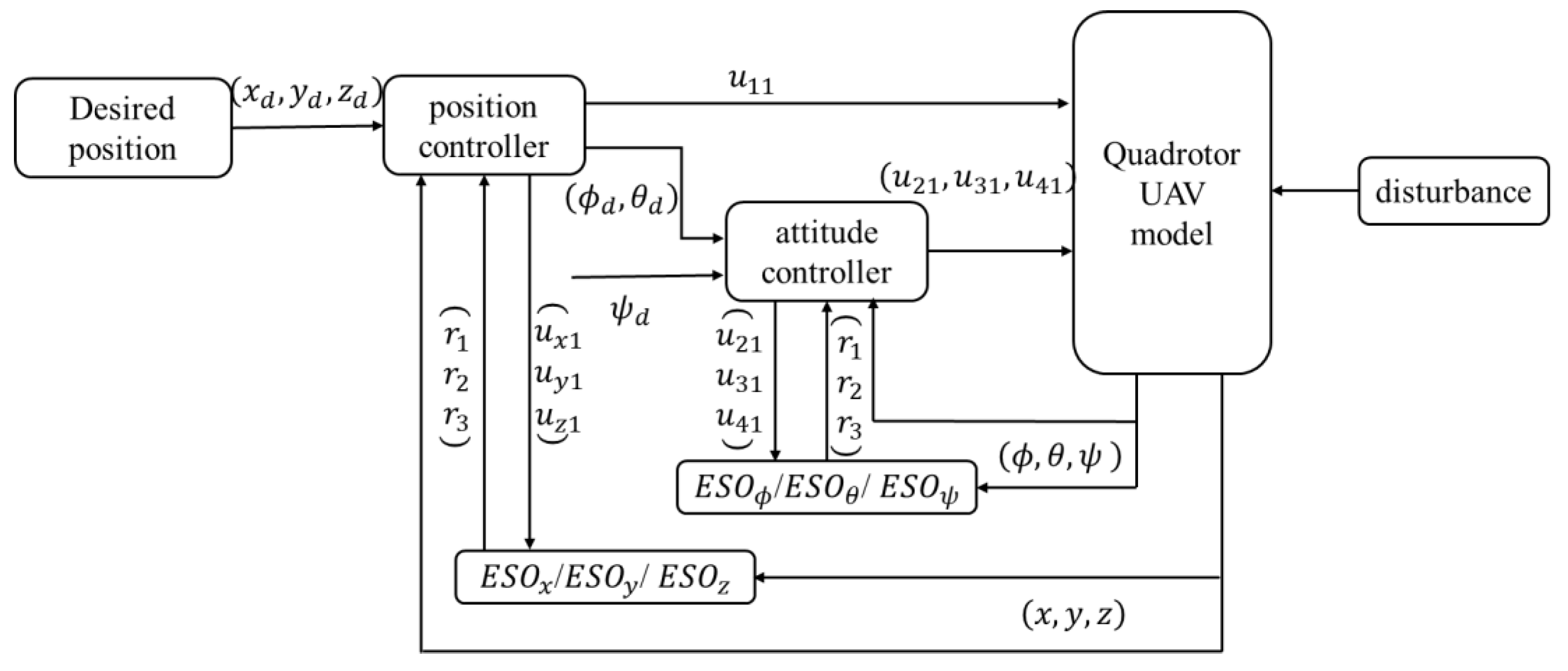
4. Design of SMC Based on ESO

Owing to the limitations of the BSC and SMC, the actual working environment of plant-protection UAVs has unknown disturbances and variable loads. Therefore, a state observer-based SMC, which does not need to add a clear disturbance model in the controller design, was developed to address this problem. When the system was disturbed, the estimated value of the disturbance was obtained through the ESO and added to the controller to solve the channel control quantity. From Equations (2) and (3), the channel control quantity of the controller is:

$$\begin{array}{c}\left\{\begin{array}{c}\begin{array}{c}{u}_{11}=b\left({\omega }_1^2+{\omega }_2^2+{\omega }_3^2+{\omega }_4^2\right) \\ u_{21}=bl\left({\omega }_4^2-{\omega }_2^2\right) \end{array}\\ \begin{array}{c}{u}_{31}=bl\left({\omega }_3^2-{\omega }_1^2\right) \\ u_{41}=d\left({\omega }_1^2+{\omega }_3^2-{\omega }_2^2-{\omega }_4^2\right)\end{array}\end{array}\right.\end{array}$$

(31)

Based on the system model of the quadrotor UAV obtained in Equations (2) and (3), the three attitude angles of the UAV were changed as follows: $u_{21}$, $u_{31}$, $u_{41}$, and $u_{11}$. The three attitude angles controlled the position of the UAV, and the position change was achieved by changing the attitude angle. Similar to the SMC and BSC, the control system of the UAV was divided into two parts to solve the underactuated problem of four inputs and six outputs: the position control of the outer loop and the attitude control of the inner loop. The control system of the quadrotor UAV is shown in Figure 4.

4.1. Position Controller Design

According to Equations (2) and (31), the decoupling of the position controller can be achieved as follows:

$$\begin{array}{c}\left\{\begin{array}{c}{u}_{x1}=u_1\left(\cos \varphi \sin \theta \cos \psi +\sin \varphi \sin \psi \right)\\ u_{y1}=u_1\left(\cos \varphi \sin \theta \cos \psi -\sin \varphi \cos \psi \right)\\ u_{z1}=u_1\left(\cos \varphi \cos \theta \right) \end{array}\right.\end{array}$$

(32)

The position control model can be obtained as:

$$\begin{array}{c}\left\{\begin{array}{c}\ddot{x}=\frac{u_{x1}}{m}+{\lambda }_x \\ \ddot{y}=\frac{u_{y1}}{m}+{\lambda }_y \\ \ddot{z}=\frac{u_{z1}}{m}-g+{\lambda }_z\end{array}\right.\end{array}$$

(33)

where ${\lambda }_x$, ${\lambda }_y$, and ${\lambda }_z$ represent the internal uncertainties in the respective channels and the total disturbance of the external disturbances.

$$\begin{array}{c}\left\{\begin{array}{c}{\dot{P}}_1=P_2 \\ {\dot{P}}_2={\ddot{P}}_1=f+bU\end{array}\right.\end{array}$$

(34)

Based on Equation (34) and taking the $x$ channel as an example for designing an ESO-based SMC as well as designing the first ESO for the $x$ channel, the observation error is defined as: $e_{x1}=r_{x1}-x$, where $r_{x1}$ represents the estimated value of $x$. Subsequently, the $ES{O}_x$ is designed as follows:

$$\begin{array}{c}\left\{\begin{array}{c}{\dot{r}}_{x1}=r_{x2}-{\beta }_1{e}_{x1} \\ {\dot{r}}_{x2}=r_{x3}-{\beta }_{2}gal\left(e_{x1},0.5\right)+u_{x1}/m \\ {\dot{r}}_{x3}=-{\beta }_{3}gal\left(e_{x1},0.25\right) \end{array}\right.\end{array}$$

(35)

where ${\beta }_1>0$, ${\beta }_2>0$, ${\beta }_3>0$; $r_{x2}$ is the estimated value of $\dot{x}$; $r_{x3}$ is the estimated value of the total disturbance ${\lambda }_x$; and the $galn$ function is used to replace the $fal$ function in the traditional ESO [24]. However, nonlinear state error feedback (NLSEF) in ADRC is essentially a PD controller, and its response speed and robustness are not as good as those of the SMC, so the combination of the improved ESO and SMC not only improves the estimation accuracy of systematic error but also retains the advantages of fast response and good robustness in the SMC. Its expression is as follows:

$$\begin{array}{c}gal\left(x,\sigma \right)=\left\{\begin{array}{c}\frac{x}{{\sigma }^2}{e}^{-\frac{{\left|x\right|}^3}{{\sigma }^2}}, \left|x\right|\le 1\\ \frac{1}{{\sigma }^2}{e}^{-\frac{1}{{\sigma }^2}}, x>1\\ -\frac{1}{{\sigma }^2}{e}^{-\frac{1}{{\sigma }^2}}, x<-1\end{array}\right.\end{array}$$

(36)

where $\sigma >0$ is the adjustable parameter of the function. When $\left|x\right|\le 1$, $gal\left(x,\sigma \right)=\frac{x}{{\sigma }^2}{e}^{-\frac{{\left|x\right|}^3}{2{\sigma }^2}}$ is a composite function, which contains an exponential function term. It can be seen that the composite function has an infinite derivative, so the function is smooth when $\left|x\right|\le 1$. According to Han J.Q. [15], a sufficiently small observation error can be achieved simply by selecting the appropriate parameters. Thus, $r_{x2}$ can replace $\dot{x}$, and $r_{x3}$ can replace the total disturbance ${\lambda }_x$.

With $x_d$ as the desired value of $x$, the sliding surface is designed as:

$$\begin{array}{c}{S}_{x1}=k_1{e}_x+{\dot{e}}_x\end{array}$$

(37)

where $k_1>0$, $e_x=x_d-x$, and ${\dot{e}}_x={\dot{x}}_d-\dot{x}$.

The exponential reaching law is also used: $\dot{S}=-\epsilon sign\left(S\right)-\rho S$, $\epsilon >0$, and $\rho >0$. Subsequently, the SMC of the x channel can be solved as:

$$\begin{array}{c}{u}_{x1}=m\left(k_1\left({\dot{x}}_d-r_{x2}\right)+{\ddot{x}}_d-r_{x3}+{\epsilon }_{x1}{S}_{x1}+{\rho }_{x1}sign\left(S_{x1}\right)\right)\end{array}$$

(38)

where ${\epsilon }_{x1}>0,$ and ${\rho }_{x1}\ge \left|k_1\left({\dot{x}}_d-r_{x2}\right)+\left({\lambda }_x-r_{x3}\right)\right|$. The error of the system converges asymptotically to zero.

The Lyapunov function and its derivative are respectively defined as:

$$\begin{array}{c}{V}_{x1}=\frac{1}{2}{S}_{x1}^2\end{array}$$

(39)

$$\begin{array}{c}{\dot{V}}_{x1}=S_{x1}{\dot{S}}_{x1}=S_{x1}\left({\ddot{x}}_d+k_1{\dot{x}}_d-k_1\dot{x}-u_{x1}/m-{\lambda }_x\right)\end{array}$$

(40)

Substituting Equation (38) for (40), we obtain:

$$\begin{array}{c}{\dot{V}}_{x1}=S_{x1}\left(k_1\left(r_{x2}-\dot{x}\right)+\left(r_{x3}-{\lambda }_x\right)-{\epsilon }_{x1}{S}_{x1}-{\rho }_{x1}sign\left(S_{x1}\right)\right)\\ \le -{\epsilon }_{x1}{S}_{x1}^2-{\rho }_{x1}\left|S_{x1}\right|+\left|S_{x1}\left(k_1\left(r_{x2}-\dot{x}\right)+\left(r_{x3}-{\lambda }_x\right)\right)\right|\end{array}$$

(41)

The designed observer $ES{O}_X$ can ensure a sufficiently small error as long as ${\rho }_{x1}$ selects an appropriate value, and ${\rho }_{x1}\ge \left|\left(k_1\left(r_{x2}-\dot{x}\right)+\left(r_{x3}-{\lambda }_x\right)\right)\right|$ at time ${\dot{V}}_{x1}\le -{\epsilon }_{x1}{S}_{x1}^2\le 0$, which satisfies the Lyapunov stability condition. Thus, the control system is stable, and the error converges asymptotically to zero.

When the models of the x, y, and z channels are similar, the controllers for the y and z channels can be designed similarly. Thus, $ES{O}_y$ is designed as:

$$\begin{array}{c}\left\{\begin{array}{c}{\dot{r}}_{y1}=r_{y2}-{\beta }_1{e}_{y1} \\ {\dot{r}}_{y2}=r_{y3}-{\beta }_{2}gal\left(e_{y1},0.5\right)+u_{y1}/m \\ {\dot{r}}_{y3}=-{\beta }_{3}gal\left(e_{y1},0.25\right) \end{array}\right. \end{array}$$

(42)

where ${\beta }_1>0$, ${\beta }_2>0$, ${\beta }_3>0$, $r_{y2}$ is the estimated value of $\dot{y}$, $r_{y3}$ is the estimated value of the total disturbance ${\lambda }_y$, and $e_{y1}=r_{y1}-y$ is the observation error variable.

Let the desired value of $y$ be $y_d$; the sliding surface is then designed as:

$$\begin{array}{c}{S}_{y1}=k_2{e}_y+{\dot{e}}_y\end{array}$$

(43)

where $k_2>0$, $e_y=y_d-y$, and ${\dot{e}}_y={\dot{y}}_d-\dot{y}$.

Subsequently, the SMC designed for the y channel is:

$$\begin{array}{c}{u}_{y1}=m\left(k_2\left({\dot{y}}_d-r_{y2}\right)+{\ddot{y}}_d-r_{y3}+{\epsilon }_{y1}{S}_{y1}+{\rho }_{y1}sign\left(S_{y1}\right)\right)\end{array}$$

(44)

where ${\epsilon }_{y1}>0,$ and ${\rho }_{y1}\ge \left|k_2\left({\dot{y}}_d-r_{y2}\right)+\left({\lambda }_y-r_{y3}\right)\right|$. The error of the system then converges asymptotically to zero.

$ES{O}_z$ is then designed as:

$$\begin{array}{c}\left\{\begin{array}{c}{\dot{r}}_{z1}=r_{z2}-{\beta }_1{e}_{z1} \\ {\dot{r}}_{z2}=r_{z3}-{\beta }_{2}gal\left(e_{z1},0.5\right)+u_{z1}/m \\ {\dot{r}}_{y3}=-{\beta }_{3}gal\left(e_{z1},0.25\right) \end{array}\right. \end{array}$$

(45)

where ${\beta }_1>0$, ${\beta }_2>0$, ${\beta }_3>0$, $r_{z2}$ is the estimated value of $\dot{z}$, $r_{z3}$ is the estimated value of the total disturbance ${\lambda }_z$, and $e_{z1}=r_{z1}-z$ is the observation error variable.

Let the desired value of $z$ be $z_d$; the sliding surface is then designed as:

$$\begin{array}{c}{S}_{z1}=k_3{e}_z+{\dot{e}}_z\end{array}$$

(46)

where $k_3>0$, $e_z=z_d-z$, and ${\dot{e}}_z={\dot{z}}_d-\dot{z}$.

The SMC designed for the y channel is:

$$\begin{array}{c}{u}_{z1}=m\left(k_3\left({\dot{y}}_d-r_{y2}\right)+{\ddot{z}}_d-r_{z3}+g+{\epsilon }_{z1}{S}_{z1}+{\rho }_{z1}sign\left(S_{z1}\right)\right)\end{array}$$

(47)

where ${\epsilon }_{z1}>0,$ and ${\rho }_{z1}\ge \left|k_3\left({\dot{z}}_d-r_{z2}\right)+\left({\lambda }_z-r_{z3}\right)\right|$. The system error converges asymptotically to zero.

The inverse solution is obtained using Equation (32), which can determine $u_{11}$, and the desired angles ${\varphi }_d$ and ${\theta }_d$ required by the inner loop.

$$\begin{array}{c}\left\{\begin{array}{c}{u}_{11}=u_{z1}/\left(\cos \varphi \cos \theta \right) \\ {\varphi }_d={\tan }^{-1}\left(\left(u_{x1}\sin \psi -u_{y1}\cos \psi \right)\cos \theta /u_{z1}\right)\\ {\theta }_d={\tan }^{-1}\left(\left(u_{x1}\cos \psi +u_{y1}\sin \psi \right)/u_{z1}\right) \end{array}\right.\end{array}$$

(48)

4.2. Attitude Controller Design

The ${\varphi }_d$ and ${\theta }_d$ from Equation (48) and the given ${\psi }_d$ are taken as the desired angle of the inner loop and used as the input for the inner loop controller. Meanwhile, $\left(I_y-I_z\right)\dot{\theta }\dot{\psi }/I_x$, $\left(I_z-I_x\right)\dot{\varphi }\dot{\psi }/I_y$, and $\left(I_x-I_y\right)\dot{\varphi }\dot{\theta }/I_z$ are used as internal disturbances estimated by the ESO. After finishing Equation (3), we can obtain:

$$\begin{array}{c}\left\{\begin{array}{c}\ddot{\varphi }=\frac{u_{21}}{I_x}+{\tilde{\lambda }}_{\varphi }\\ \ddot{\theta }=\frac{u_{31}}{I_x}+{\tilde{\lambda }}_{\theta }\\ \ddot{\psi }=\frac{u_{41}}{I_z}+{\tilde{\lambda }}_{\psi }\end{array}\right.\end{array}$$

(49)

where ${\tilde{\lambda }}_{\varphi }=\left(I_y-I_z\right)\dot{\theta }\dot{\psi }/I_x+{\lambda }_{\varphi }$, ${\tilde{\lambda }}_{\theta }=\left(I_z-I_x\right)\dot{\varphi }\dot{\psi }/I_y+{\lambda }_{\theta }$, and ${\tilde{\lambda }}_{\psi }=\left(I_x-I_y\right)\dot{\varphi }\dot{\theta }/I_z+{\lambda }_{\psi }$ are the total disturbances of each channel of the inner loop.

Similar to the design process of the outer-loop controller, the inner-loop attitude controller is designed. The $\varphi$ channel $ES{O}_{\varphi }$ is designed as:

$$\begin{array}{c}\left\{\begin{array}{c}{\dot{r}}_{\varphi 1}=r_{\varphi 2}-{\beta }_4{e}_{\varphi 1} \\ {\dot{r}}_{\varphi 2}=r_{\varphi 3}-{\beta }_{5}gal\left(e_{\varphi 1},0.5\right)+u_{21}/I_x \\ {\dot{r}}_{\varphi 3}=-{\beta }_{6}gal\left(e_{\varphi 1},0.25\right) \end{array}\right.\end{array}$$

(50)

where ${\beta }_4>0$, ${\beta }_5>0$, ${\beta }_6>0$, $r_{\varphi 2}$ is the estimated value of $\dot{\varphi }$, $r_{\varphi 3}$ is the estimated value of the total disturbance ${\tilde{\lambda }}_{\varphi }$, and $e_{\varphi 1}=r_{\varphi 1}-\varphi$ is the observation error variable.

Let the desired value of $\varphi$ be ${\varphi }_d$; the sliding surface is then designed as:

$$\begin{array}{c}{S}_{\varphi 1}=k_4{e}_{\varphi }+{\dot{e}}_{\varphi }\end{array}$$

(51)

where $k_4>0$, $e_{\varphi }={\varphi }_d-\varphi$, and ${\dot{e}}_{\varphi }={\dot{\varphi }}_d-\dot{\varphi }$.

The SMC designed for the $\varphi$ channel is:

$$\begin{array}{c}{u}_{21}=I_x\left(k_4\left({\dot{\varphi }}_d-r_{\varphi 2}\right)+{\ddot{\varphi }}_d-r_{\varphi 3}+{\epsilon }_{\varphi 1}{S}_{\varphi 1}+{\rho }_{\varphi 1}sign\left(S_{\varphi 1}\right)\right)\end{array}$$

(52)

where ${\epsilon }_{\varphi 1}>0,$ and ${\rho }_{\varphi 1}\ge \left|k_4\left({\dot{\varphi }}_d-r_{\varphi 2}\right)+\left({\tilde{\lambda }}_{\varphi }-r_{\varphi 3}\right)\right|$. The system error converges asymptotically to zero.

$ES{O}_{\theta }$ is then designed as:

$$\begin{array}{c}\left\{\begin{array}{c}{\dot{r}}_{\theta 1}=r_{\theta 2}-{\beta }_4{e}_{\theta 1} \\ {\dot{r}}_{\theta 2}=r_{\theta 3}-{\beta }_{5}gal\left(e_{\theta 1},0.5\right)+u_{31}/I_y \\ {\dot{r}}_{\theta 3}=-{\beta }_{6}gal\left(e_{\theta 1},0.25\right) \end{array}\right.\end{array}$$

(53)

where ${\beta }_4>0$, ${\beta }_5>0$, ${\beta }_6>0$, $r_{\theta 2}$ is the estimated value of $\dot{\theta }$, $r_{\theta 3}$ is the estimated value of the total disturbance ${\tilde{\lambda }}_{\theta }$, and $e_{\theta 1}=r_{\theta 1}-\theta$ is the observation error variable.

The desired value of $\theta$ is ${\theta }_d$, and the sliding surface is designed as:

$$\begin{array}{c}{S}_{\theta 1}=k_5{e}_{\theta }+{\dot{e}}_{\theta }\end{array}$$

(54)

where $k_5>0$, $e_{\theta }={\theta }_d-\theta$, and ${\dot{e}}_{\theta }={\dot{\theta }}_d-\dot{\theta }$.

The SMC designed for the $\theta$ channel is:

$$\begin{array}{c}{U}_3=I_y\left(k_5\left({\dot{\theta }}_d-r_{\theta 2}\right)+{\ddot{\theta }}_d-r_{\theta 3}+{\epsilon }_{\theta 1}{S}_{\theta 1}+{\rho }_{\theta 1}sign\left(S_{\theta 1}\right)\right)\end{array}$$

(55)

where ${\epsilon }_{\theta 1}>0,$ and ${\rho }_{\theta 1}\ge \left|k_5\left({\dot{\theta }}_d-r_{\theta 2}\right)+\left({\tilde{\lambda }}_{\theta }-r_{\theta 3}\right)\right|$. The system error converges asymptotically to zero.

$ES{O}_{\psi }$ is then designed as:

$$\begin{array}{c}\left\{\begin{array}{c}{\dot{r}}_{\psi 1}=r_{\psi 2}-{\beta }_4{e}_{\psi 1} \\ {\dot{r}}_{\psi 2}=r_{\psi 3}-{\beta }_{5}gal\left(e_{\psi 1},0.5\right)+u_{41}/I_z \\ {\dot{r}}_{\psi 3}=-{\beta }_{6}gal\left(e_{\psi 1},0.25\right) \end{array}\right.\end{array}$$

(56)

where, ${\beta }_4>0$, ${\beta }_5>0$, ${\beta }_6>0$, $r_{\psi 2}$ is the estimated value of $\dot{\psi }$, $r_{\psi 3}$ is the estimated value of the total disturbance ${\tilde{\lambda }}_{\psi }$, and $e_{\psi 1}=r_{\psi 1}-\psi$ is the observation error variable.

The desired value of $\psi$ is ${\psi }_d$, and the sliding surface is then designed as:

$$\begin{array}{c}{S}_{\psi 1}=k_6{e}_{\psi }+{\dot{e}}_{\psi }\end{array}$$

(57)

where $k_6>0$, $e_{\psi }={\psi }_d-\psi$, and ${\dot{e}}_{\psi }={\dot{\psi }}_d-\psi$.

The SMC designed for the $\psi$ channel is:

$$\begin{array}{c}{U}_4=I_z\left(k_6\left({\dot{\psi }}_d-r_{\psi 2}\right)+{\ddot{\psi }}_d-r_{\psi 3}+{\epsilon }_{\psi 1}{S}_{\psi 1}+{\rho }_{\psi 1}sign\left(S_{\psi 1}\right)\right)\end{array}$$

(58)

where ${\epsilon }_{\psi 1}>0,$ and ${\rho }_{\psi 1}\ge \left|k_6\left({\dot{\psi }}_d-r_{\psi 2}\right)+\left({\tilde{\lambda }}_{\psi }-r_{\psi 3}\right)\right|$. The system error converges asymptotically to zero.

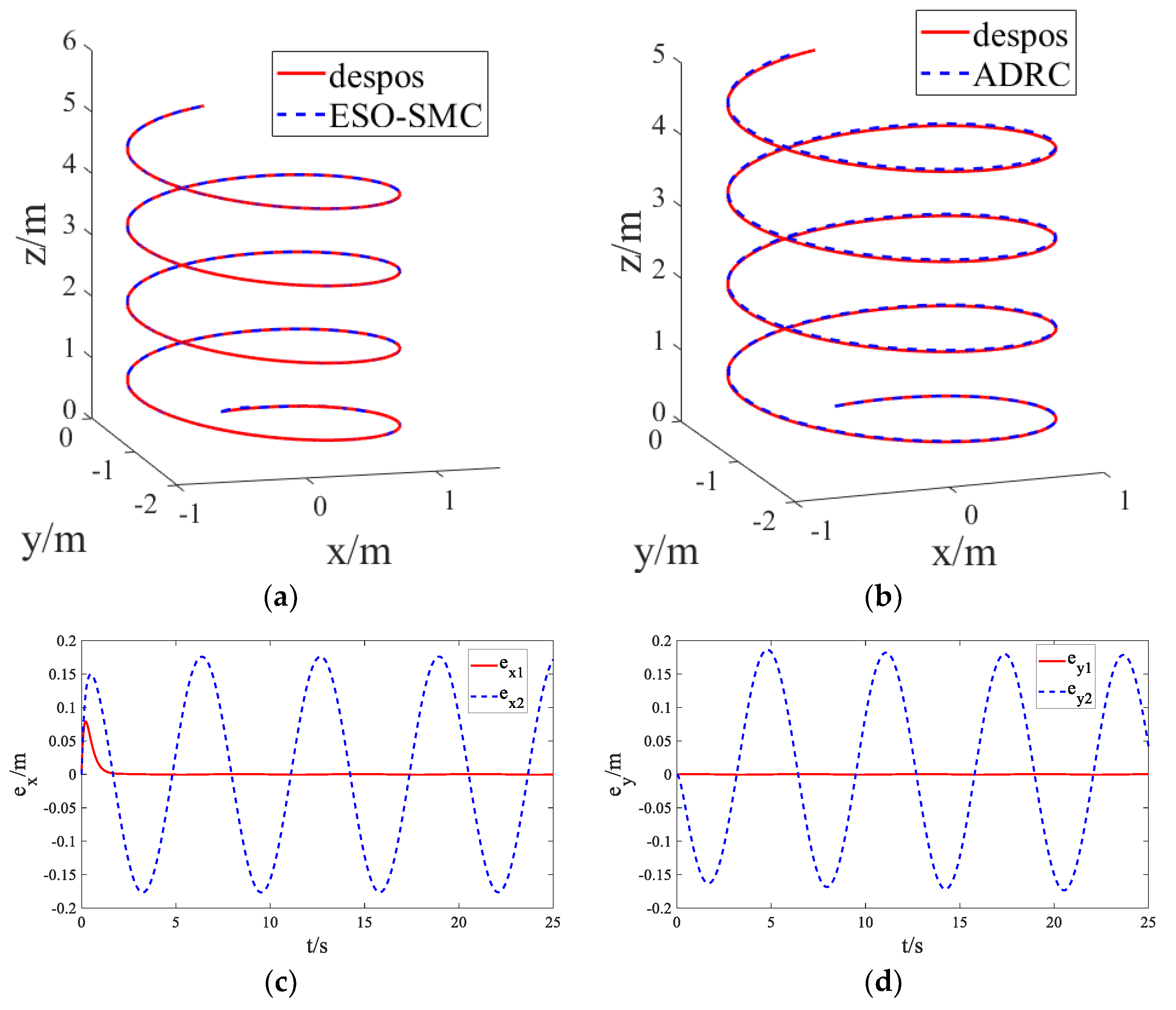
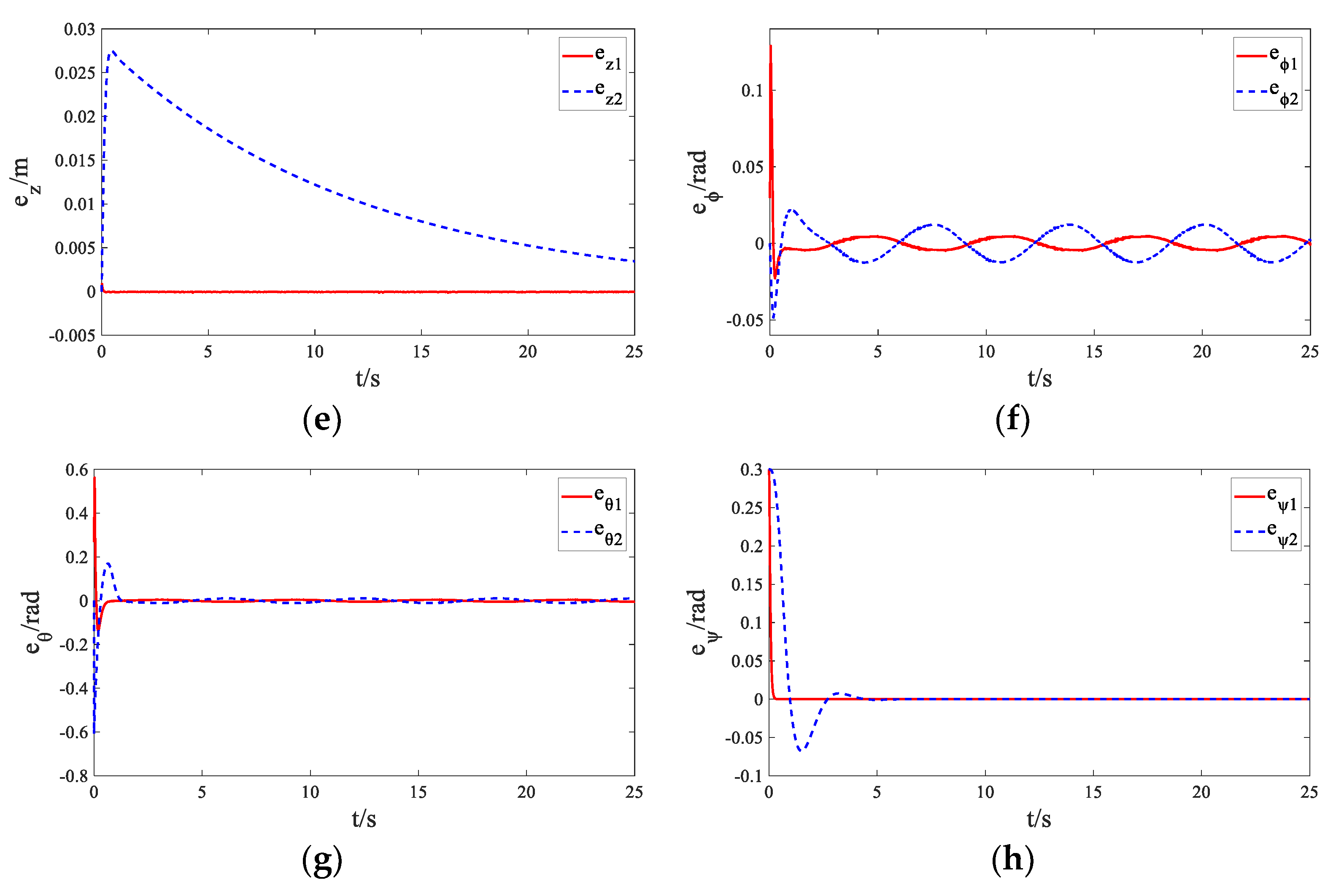
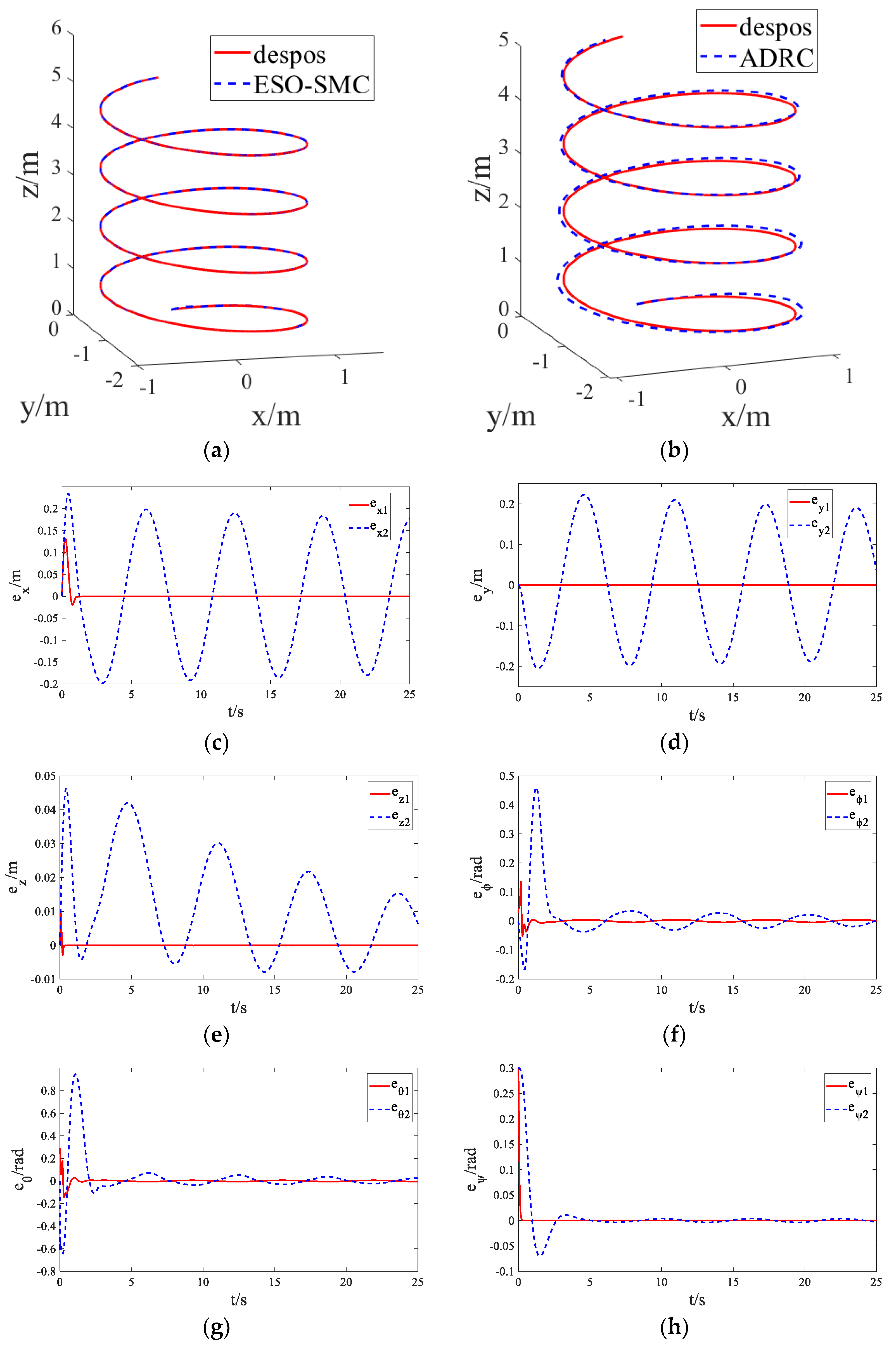
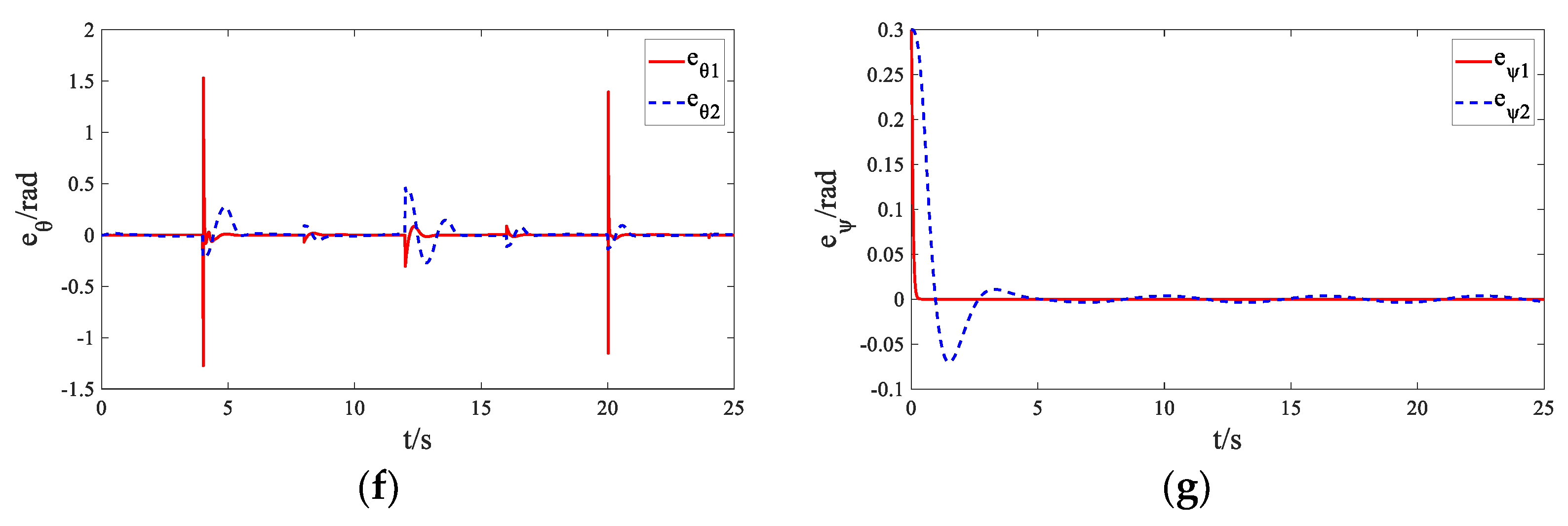
4.3. Simulation Analysis

In the simulation experiment, the parameters were set as follows: $k_1=k_2=3.5$, $k_3=35$, ${\epsilon }_{x1}={\epsilon }_{x2}=4$, ${\epsilon }_{x3}=75$, ${\rho }_{x1}={\rho }_{x2}=1.5$, ${\rho }_{x3}=10$, ${\beta }_1=100$, ${\beta }_2=510$, ${\beta }_3=2000$, $k_4=k_5=k_6=25$, ${\epsilon }_{\varphi 1}={\epsilon }_{\theta 1}={\epsilon }_{\psi 1}=35$, ${\rho }_{\varphi 1}={\rho }_{\theta 1}={\rho }_{\psi 1}=4.5$, ${\beta }_4=200$, ${\beta }_5=800$, and ${\beta }_6=3000$. The desired trajectory was set as $x_d=\sin t$, $y_d=\cos t-1$, and $z_d=0.2t$, and the desired angle was set as ${\psi }_d=0.3$. Assuming zero external disturbances except for the external disturbance of the inner ring, the initial data of the quadrotor UAV were: ${\left[x y z \varphi \theta \psi \right]}^T={\left[0 0 0 0 0 0\right]}^T$. The simulation was performed using MATLAB/Simulink with the simulation time set to 25 s. The results were compared with those of traditional ADRC. The simulation results are shown in Figure 5.

In Figure 5c–h, $e_{i1}\left(i=x,y,z,\varphi ,\theta ,\psi \right)$ are the channel errors of the ESO−SMC, and $e_{i2}\left(i=x,y,z,\varphi ,\theta ,\psi \right)$ is the channel error of ADRC. Without external disturbance, the ESO−SMC had the fastest tracking speed, and the tracking error tended to stabilize to zero within 1 s, whereas ADRC had a slightly slower response speed. In addition, the effect of the position control and BSC were similar, whereas the angle control of the ESO−SMC was better than that of ADRC. Compared with ADRC, the ESO−SMC had better tracking accuracy and stability. Overall control performance has been improved.

Plant−protection UAVs can determine spraying concentration according to the information returned by the camera. As the simulation only needs to verify the anti-interference ability of the controller, an equal spraying concentration of the pesticide was assumed, that is, the change in quality is the same as time: $M=3-0.1t$, which is added to the quadrotor UAV system as a disturbance. The desired trajectory was still set as: $x_d=\sin t$, $y_d=\cos t-1,$ and $z_d=0.2t$, and the desired angle was ${\psi }_d=0.3$. In addition to the load disturbance, the disturbances applied by the position loop were: $\left[\begin{array}{ccc}0.3\sin t& 0.3\sin t& 0.3\sin t\end{array}\right]$, and the disturbances applied by the attitude loop were: $\left[\begin{array}{ccc}0.2\sin t& 0& 0.3\sin t\end{array}\right]$. The initial data of the quadrotor UAV were: ${\left[x y z \varphi \theta \psi \right]}^T={\left[0 0 0 0 0 0\right]}^T$. The simulation was performed using MATLAB/Simulink with the time set to 25 s. The results were compared with that of the traditional ADRC. The simulation results are shown in Figure 6.

Even with the additions of variable load and external disturbance, the ESO−SMC can still quickly track the desired target, and the tracking error was reduced and stabilized to approximately 0 within 1 s, as shown in Figure 6. ADRC exhibited a slightly slower response speed that can estimate the error well and achieve tracking. Compared with the undisturbed case, the z-axis error gradually fluctuated as the load decreased, and the angle control also slightly fluctuated. The ESO−SMC improved the robustness, tracking accuracy, and stability of the system. Overall control performance has been improved.

The disturbance is the same as above, and the desired trajectory was as follows: when $0\le t\le 4$, $x_d=0$, $y_d=0$, $z_d=0.5t$; when $4<t\le 8$, $x_d=0.5\left(t-4\right)$, $y_d=0$, $z_d=2$; when $8<t\le 12$, $x_d=2$, $y_d=t-8$, and $z_d=2$; $12<t\le 16$, $x_d=2-0.5\left(t-12\right)$, $y_d=4$, and $z_d=2$; $16<t\le 20$, $x_d=0$, $y_d=4-\left(t-16\right)$, and $z_d=2$; $20<t\le 24$, $x_d=0$, $y_d=0$, and $z_d=2-0.5\left(t-20\right)$; and $24<t\le 25$, and $x_d=y_d=z_d=0$. The desired angle was ${\psi }_d=0.3$. The initial data of the quadrotor UAV were: ${\left[x y z \varphi \theta \psi \right]}^T={\left[0 0 0 0 0 0\right]}^T$. The simulation was carried out using MATLAB/Simulink with the time set to 25 s. The results were compared with that of the traditional ADRC. The simulation results are shown in Figure 7.

The tracking speed of the ESO−SMC was faster than that of ADRC, whereby the tracking error was highly stable as it approached 0 within 1 s. Meanwhile, the response speed of ADRC was slightly slower, the error changed within a large range, and it was difficult to stabilize the error at 0 point. Thus, the ESO−SMC improved the robustness, tracking accuracy, and stability of the system. Overall control performance has been improved.

5. Conclusions

In this study, the control system is decomposed into two parts (the outer-loop position control and the inner-loop attitude control) for the underactuated system of a quadrotor UAV. With a view toward the practical application of UAVs in plant protection, an SMC based on the ESO was designed considering load change and unknown external disturbance. When the plant-protection UAV is designed under interference, its tracking error can be reduced to 0 within 1 s and remain stable. However, the error of ADRC fluctuates greatly, error stabilization takes about 4S, and it is difficult to stabilize at 0. Simulation and comparison experiments show that the tracking error is stably shortened by more than 3S, the average error is reduced by more than 50%, the tracking response speed is significantly improved, the tracking error is significantly reduced, and stability is enhanced. It shows that the controller can improve the anti-interference ability, tracking speed, tracking error, fluctuation amplitude, robustness, and flight stability of the system. The overall control performance is significantly improved.

References

1. Kocer, B.B.; Tjahjowidodo, T.; Seet, G.G.L. Centralized predictive ceiling interaction control of quadrotor VTOL UAV. Aerosp. Sci. Technol. 2018, 76, 455–465. [Google Scholar] [CrossRef]
2. Du, B.H.; Polyakov, A.; Zheng, G.; Quan, Q. Quadrotor trajectory tracking by using fixed-time differentiator. Int. J. Control 2018, 92, 2854–2868. [Google Scholar] [CrossRef] [Green Version]
3. Wang, C.; Yang, J.; Yao, H.; Xi, J. Overview of flight control algorithms for quadrotor UAV. Electro. Opt. Control. 2018, 25, 57–62. [Google Scholar]
4. Wang, H.Y.; Zhao, J.K.; Yu, W.X.; Tian, W.F. Modelling and position tracking control for quadrotor vehicle. J. Chin. Inert. Technol. 2012, 20, 455–489. [Google Scholar]
5. Badr, S.; Mehrez, O.; Kabeel, A.E. A design modification for a quadrotor UAV: Modeling, control and implementation. Adv. Robot. 2019, 33, 13–32. [Google Scholar] [CrossRef]
6. Li, Y.B.; Song, S.X. Hovering control of PID four-rotor UAV based on fuzzy self-tuning. Control. Eng. 2013, 20, 910–914. [Google Scholar]
7. Zuo, Z.Y.; Mallikarjunan, S.L. adaptive backstepping for robust trajectory tracking of UAVs. IEEE Trans. Ind. Electron. 2017, 64, 2944–2954. [Google Scholar] [CrossRef]
8. Djamel, K.; Abdellah, M.; Benallegue, A. Attitude optimal backstepping controller-based quaternion for a UAV [J/OL] Mathematical Problems in Engineering. Math. Probl. Eng. 2016, 2016, 1–11. [Google Scholar] [CrossRef] [Green Version]
9. Yin, C.; Huang, X.; Chen, Y.; Dadras, S.; Zhong, S.M.; Cheng, Y. Fractional-order exponential switching technique to enhance sliding mode control. Appl. Math. Model. 2017, 44, 705–726. [Google Scholar] [CrossRef]
10. Labbadi, M.; Cherkaoui, M. Robust adaptive backstepping fast terminal sliding mode controller for uncertain quadrotor UAV. Aerosp. Sci. Technol. 2019, 93, 105306. [Google Scholar] [CrossRef]
11. Zheng, Z.; Fang, W.; Ying, G.; Hua, C. Multivariable sliding mode backstepping controller design for quadrotor UAV based on disturbance observer. Sci. China 2018, 61, 155–170. [Google Scholar] [CrossRef]
12. Chen, F.Y.; Jiang, R.Q.; Zhang, K.K.; Jiang, B.; Tao, G. Robust backstepping sliding-mode control and observer-based fault estimation for a quadrotor UAV. IEEE Trans. Ind. Electron. 2016, 63, 5044–5056. [Google Scholar] [CrossRef]
13. Jeong, S.; Chwa, D. Coupled multiple sliding-mode control for robust trajectory tracking of hovercraft with external disturbances. IEEE Trans. Ind. Electron. 2018, 65, 4103–4113. [Google Scholar] [CrossRef]
14. Shao, X.L.; Liu, J.; Cao, H.L.; Shen, C.; Wang, H. Robust dynamic surface trajectory tracking control for a quadrotor UAV via extended state observer. Int. J. Robust Nonlinear Control. 2018, 28, 2700–2719. [Google Scholar] [CrossRef]
15. Han, J.Q. From PID to active disturbance rejection control. IEEE Trans. Ind. Electron. 2009, 56, 900–906. [Google Scholar] [CrossRef]
16. Cheng, Y.; Chen, Z.Q.; Sun, M.W.; Sun, Q. Multivariable-inverted decoupling active disturbance rejection control and its application to a distillation column process. Acta Autom. Sin. 2017, 43, 1080–1088. [Google Scholar]
17. Zheng, Q.; Gao, Z. Active disturbance rejection control: Some recent experimental and industrial case studies. Control. Theory Technol. 2018, 16, 301–313. [Google Scholar] [CrossRef]
18. Wu, Y.J.; Li, C.; Ma, Z. Triaxial flexible satellite attitude control based on active disturbance rejection sliding mode. J. Syst. Simul. 2015, 27, 1831–1837. [Google Scholar]
19. Li, D.Y.; Li, Z.; Jin, Q. ADRC method based on linear state feedback and higher-order Taylor approximation. Control. Decis. 2015, 30, 166–170. [Google Scholar]
20. Shao, X.L.; Wang, H. Performance analysis of linear extended state observer and its higher-order form. Control. Decis. 2015, 30, 815–822. [Google Scholar]
21. Liu, B.; Qiu, B.; Cui, Y.; Sun, J. Fault-tolerant H ∞ control for net-worked control systems with randomly occurring missing measurements. Neurocomputing 2016, 17, 459–465. [Google Scholar] [CrossRef]
22. Zhang, Y.; Chen, Z.; Zhang, X.; Sun, Q.; Sun, M. A Novel Control Scheme for Quadrotor UAV Based upon Active Disturbance Rejection Control. Aerosp. Sci. Technol. 2018, 79, 601–609. [Google Scholar] [CrossRef]
23. Li, J.; Li, Y. Modeling and PID control for a quadrotor. J. Liaoning Tech. Univ. 2012, 1, 114–117. [Google Scholar]
24. Yang, W.Q.; Lu, J.H.; Jiang, X.; Wang, Y.X. Design of quadrotor attitude active disturbance rejection controller based on improved ESO[J/OL], Systems Engineering and Electronics. In Proceedings of the 2021 3rd International Academic Exchange Conference on Science and Technology Innovation (IAECST), Guangzhou, China, 10–12 December 2021. [Google Scholar]
Figure 1. Diagram of the movement of the quadrotor UAV.
Mathematics 10 01346 g001
Figure 2. Control system of the quadrotor UAV based on SMC.
Mathematics 10 01346 g002
Figure 3. Error comparison of the trajectory−tracking based on BSC and SMC without disturbance: (a) 3D effect; (b) x trajectory; (c) y trajectory; (d) z trajectory; (e) roll angle; (f) pitch angle; and (g) yaw angle.
Mathematics 10 01346 g003
Figure 4. Control system of the quadrotor UAV based on ESO-SMC.
Mathematics 10 01346 g004
Figure 5. Comparison of the trajectory−tracking errors based on ESO−SMC and ADRC without disturbance: (a) ESO−SMC 3D effect; (b) ADRC 3D effect; (c) x trajectory; (d) y trajectory; (e) z trajectory; (f) roll angle; (g) pitch angle; and (h) yaw angle.
Mathematics 10 01346 g005aMathematics 10 01346 g005b
Figure 6. Comparison of the trajectory−tracking errors based on ESO−SMC and ADRC under disturbance: (a) ESO−SMC 3D effect; (b) ADRC 3D effect; (c) x trajectory; (d) y trajectory; (e) z trajectory; (f) roll angle; (g) pitch angle; and (h) yaw angle.
Mathematics 10 01346 g006
Figure 7. Comparison of the trajectory−tracking errors based on ESO−SMC and ADRC under disturbance: (a) 3D effect; (b) x trajectory; (c) y trajectory; (d) z trajectory; (e) roll angle; (f) pitch angle; and (g) yaw angle.
Mathematics 10 01346 g007aMathematics 10 01346 g007b
Publisher’s Note: MDPI stays neutral with regard to jurisdictional claims in published maps and institutional affiliations.