Abstract
In this paper, a transmission expansion planning (TEP) model is proposed to guarantee the resilience of power systems and mitigate cascading failures’ impacts. The energy storage systems and fault current limiters’ planning models are integrated into the TEP problem to minimize cascading outages and comply with short-circuit current reliability constraints. Most studies in the literature adopt a single strategy to simulate power systems’ cascading failures that may not be enough to guarantee networks’ resilience. This work elaborates on two scenarios for initiating cascading failures to study the impact of various initiating events on the planned system’s strength and the projects required. The TEP problem is formulated as a non-linear, non-convex large-scale problem. To avoid linearization issues and enhance meta-heuristics performance, a hybridization of two meta-heuristic techniques, namely snake optimizer and sine cosine algorithm (SO-SCA), is proposed to solve the problem. Two hybridization strategies are suggested to improve the exploration and exploitation stages. Defining future loads growth is essential for TEP. Hence, a load forecasting technique based on SO-SCA is investigated and compared with some methods reported in the literature. The results obtained proved the efficiency of the proposed approach in predicting load growth. TEP’s calculations were carried out on the Garver and the IEEE 24-bus system. The results demonstrated the superiority of the hybrid SO-SCA in solving the TEP problem. Moreover, the projects required to expand networks differed according to the type of cascading failures’ initiating scenario.
Keywords:
transmission expansion planning; cascading failures; meta-heuristic technique; load forecasting MSC:
90-08
1. Introduction
The transmission expansion planning (TEP) problem corresponds to allocating different power facilities, such as transmission lines, energy storage systems (ESSs), thyristor-controlled series compensators (TCSC), and fault current limiters (FCLs), to satisfy the expected load growth and fulfill operational and reliability constraints [1]. TEP is a well-studied problem in the literature; however, there are still many challenges related to solution methods and offering a mathematical model that can accommodate the power system’s uncertainties and ensure reliability constraints [2].
Several mathematical, heuristic and meta-heuristic methods were reported in the literature to solve TEP models [2]. Some of these works are introduced below as follows. In Hamidpour et al. [3], the AC power flow-based model (ACTEP) was adopted. The non-linear and non-convex constraints were linearized through Taylor’s expansion and polygon approaches. The CPLEX solver solved the linearized model within GAMS. The suggested strategy was conducted on the IEEE 6-bus and 30-bus test systems. The numerical results verified the efficiency of the proposed solution. Esmaili et al. [4] presented a Benders’ decomposition approach that included a successive linearization technique to solve a multi-stage TEP problem and deal with non-linear constraints. The integration of thyristor TCSCs and FCLs’ allocation problem with the TEP problem increased the problem’s complexity and non-linearity. The proposed method was tested on the IEEE 39- and 118-bus systems. Solvers like GUROBI and CONOPT were used to solve the proposed model. The suggested strategy demonstrated its superiority in terms of linearization error and execution time measured. Franken et al. [5] developed an approach based on the DC power flow-based(DCTEP) model for the simultaneous incorporation of TEP and planning problems of TCSCs, phase-shifting transformers, and high voltage direct current systems (HVDC). The problem was translated into a mixed-integer linear programming model (MILP), and the solver CPLEX within the MATLAB platform was used to solve the problem. In Moradi-Sepahvand et al. [6], a MILP was investigated to formulate TEP integrated HVDC, HVACs, and ESSs in the presence of renewable energy sources. The problem was divided into a master problem and sub-problems and was solved using the CPLEX solver in GAMS. To validate the suggested approach, different test cases were carried out on the Garver network, IEEE 24-bus system, and IEEE 118-bus system.
Regarding the implementation of meta-heuristic techniques, sine cosine algorithm (SCA), Levy flight optimizer (LFO), and the linear population size reduction—success-history-based differential evolution with semi-parameter adaptation hybrid—covariance matrix adaptation evolution strategy algorithm (LSHADE-SPACMA) were tested in Refaat et al. [7] to solve the TEP problem and FCLs allocation problem. DCTEP was formulated, and SCA proved its superiority in obtaining high-quality solutions with a reasonable execution time. In Abdi et al. [8], different algorithms, such as a genetic algorithm, an orthogonal crossover-based differential evolution, grey wolf optimizer, moth–flame optimization, exchange market algorithm, SCA, and imperialistic competitive algorithm, were examined to solve the TEP problem. A comparative analysis was done using the 24 and 118 benchmark systems. The numerical results of different scenarios showed that the grey wolf optimizer was recommended for solving the TEP problem. The non-dominated sorting genetic algorithm II-based Pareto approach was investigated by Abbasi et al. [9] to solve a multi-objective DCTEP problem. The obtained results over two test systems proved the efficiency of the applied technique in dealing with non-linearity in the adopted model.
Meta-heuristic algorithms perform differently in different types of problems. One may perform slightly better than the other in a particular problem and worse in other sets of problems [2]. Further, the success of meta-heuristics mainly hinges on the encoding of candidate solutions and thus the search space. Nowadays, many studies encourage the hybridization of several techniques in one algorithm to overcome these issues. Refaat et al. [7] suggested an approach that combined mathematical and meta-heuristic techniques to solve TEP. A stochastic planning model that considered short-circuit constraints and N-1 security was adopted. The problem was translated into a three-level problem. In the first level, a meta-heuristic algorithm was applied to place new circuits and FCLs such that short-circuit current constraint was achieved. Two mathematical techniques were employed in the second and third stages to decide the best location for new generation units to meet power flow constraints during steady-state operation and define the load shedding to satisfy N-1 reliability during contingencies. The results proved the suggested strategy for handling non-linear constraints and improving the performance of meta-heuristic techniques. Ramachandran et al. [10] proposed an algorithm combining the modified grasshopper optimizer and the improved Harris hawks optimization algorithm to balance the global search and global convergence phases. The results ascertained the capability of the proposed algorithm in providing promising results compared with some algorithms presented in the literature. The hybrid Harris hawks optimizer-arithmetic optimization algorithm was proposed by Cetinbas et al. [11] for autonomous micro-grids design and sizing. The results proved the efficiency of the algorithm suggested. A hosting capacity planning model was developed by Almalaq et al. [12] to increase the use of RESs. A hybrid of two meta-heuristic techniques was employed to deal with non-convexities within the search space. The results showed the effectiveness of the suggested approach in enhancing the exploration and exploitation stages and getting high-quality solutions.
A heuristic approach based on fuzzy logic was developed by Sousa et al. [13] for TEP. The simulation results carried out on different test systems confirmed the proposed technique’s effectiveness in finding high-quality solutions. In Armaghani et al. [14], an analytical multi-stage TEP approach combined with a forward pseudo-dynamic planning method was proposed for finding critical transmission lines that may initiate and propagate the cascading failure.
Recently, cascading failures’ impacts during TEP have been taken into account in several studies [15,16,17]. Mehrtash et al. [15] contributed to a risk-based planning model that minimizes cascading failures’ effects. The suggested problem was modeled as a mixed-integer second-order cone programming problem. Risk indices were considered in the developed model to measure the non-identical probability and individual contingencies’ consequences. The results obtained from the IEEE 24-bus system demonstrated that the system planned was more robust against high-risk contingencies that may have resulted in cascading failures. Qorbani et al. [16] developed a resilient TEP model to mitigate cascading outages’ effects and ensure N-1 security. The outage of two-connected lines to each node was the triggering event for cascading failures. Gjorgiev et al. [17] proposed a risk-informed TEP method. An AC-based cascading failure model was developed to simulate post contingencies power systems’ responses. A multi-objective optimization was investigated and solved using a meta-heuristic algorithm. The suggested procedure succeeded in mitigating the effects of cascading failures.
Calculation of future peak loads is essential for TEP; hence the accuracy of the load forecasting tool implemented is necessary to guarantee the accuracy of the planning process. The hyper-parameters of the forecasting models play an essential role in improving the model’s performance [18,19,20,21]. A long-term load prediction-based particle swarm optimization was implemented by AlRashidi et al. [21]. The results demonstrated the superiority of the applied optimizer in estimating forecasting models’ parameters compared to the least error square method. An adaptive neural fuzzy system was recommended by Fathy et al. [22] and Refaat et al. [23] as an efficient tool for load forecasting. However, it had a problem selecting the type and the number of membership functions. Hong et al. [24] applied the support vector machines method to forecast future loads growth; however, it has parameters selection problems. In this work, a load forecasting approach based on a hybrid of two-meta heuristic techniques is proposed and compared with some methods presented in the literature.
Based on all the above discussion, the existing research gaps are illustrated as follows:
- The mathematical methods efficiently solve linear and simple TEP problems. However, they need a high computational burden for solving large-scale non–linear TEP problems with a vast search space. These methods have difficulty finding the optimal solution, mainly if non-convexities exist with the search space. Most of the existing works apply a linearization scheme and a decomposing strategy to simplify the problem, but it may result in linearization errors that affect the accuracy of obtained solutions.
- As known, the meta-heuristics are not transparent algorithms. They are time-consuming and challenging to reach the optimal solution in a single run [2]. Much effort is still needed for improving the performance of meta-heuristic techniques in solving TEP problems.
- Although heuristic methods need a lower computational burden compared to mathematical and meta-heuristic algorithms, they cannot guarantee the optimal solution or high-quality solutions.
- The hybridization of several optimization algorithms is recommended for solving the TEP problems. However, most current studies proposed it for solving the DCTEP problem that is simple compared to the AC models. Testing the performance of the hybrid algorithms in solving the ACTEP problems is rarely discussed in the literature.
- Most existing works simulate a single strategy to avoid cascading failures of power systems that may not be enough to ensure the electrical networks’ resilience and security.
- Most current research adopts a single optimization algorithm to calculate future loads in the long term. However, the hybrid implementation of several meta-heuristic algorithms is rarely examined in the literature.
This work corresponds to introducing a robust TEP model and investigating a long-term load forecasting method to address the mentioned shortcomings. The ACTEP is adopted in this work. It handles short-circuit current constraints and cascading failures impacts. The proposed model is non-linear and non-convex. To avoid linearization, a hybrid of two meta-heuristic algorithms is developed. The main contributions of this study can be outlined as follows:
- The meta-heuristic algorithm, Snake optimizer (SO) [25], is combined with the sine cosine algorithm (SCA) [26] to solve the proposed TEP problem and calculate the long-term load forecasting. Two combination approaches are adopted to enhance both algorithms’ exploration and exploitation phases.
- The use of renewable energy sources (RESs) threatens the modern power systems’ resilience and may be a trigger to cascading failures and rolling blackouts [27,28]. Therefore, the adopted model deals with RESs’ stochastic behavior.
- Two scenarios for initiating cascading failures are suggested to ensure the planned system’s strength and study the impact of various initiating events on the projects required.
- The impact of ESSs and FCLs in minimizing cascading outages and fulfilling short-circuit current constraints is also investigated. In this regard, Sodium sulfur batteries (NaS) and FCLs’ sizing and placing problems are included in the TEP problem.
2. Problem Formulation
The TEP problem is modeled as an optimization problem to expand power networks, increase networks’ resilience and achieve reliability constraints in the presence of RESs. The proposed objective function targets to minimize the cost of installed circuits, FCLs, generation units and ESSs.
The AC model is adopted in this study to formulate the proposed problem. It is superior to the DC model in terms of the accuracy of the results obtained and the ability to integrate many problems into a single model, such as combining the problem of reactive power units’ allocation and the TEP into a single problem [27]. A clustered data of wind speed and load consumed over the year simulate power systems’ stochastic behavior.
As mentioned before, TEP is always linked to future loads; therefore, implementing an accurate load forecasting technique is essential to improve the planning process. In this regard, the load forecasting problem is formulated as an estimation process, and the hybrid of SO-SCA is applied to minimize the error associated with the estimated model.
2.1. Mathematical Model of TEP
The proposed TEP model has a single objective function and is subjected to normal and security constraints, as illustrated in (1)–(29). Equation (1) provides the proposed cost function. The first term concerns the cost of installed circuits, while the second and third terms cover the cost of FCLs and NaS batteries required to achieve security and short-circuit current constraints. The fourth term covers the cost of new generation units installed. The reminder terms present the operating cost of NaS batteries and thermal units and RESs, respectively.
where the recovery factor is inserted in the cost function to consider the money’s time value [29], where and are the discount rate and the lifetime of the project in years, respectively. The problem constraints are provided in (2)–(29). The steady-state constraints are shown in (2)–(24), whereas reliability constraints are given in (25)–(29). Constraints (2) and (3) are related to active and reactive powers injected at each node. is negative if an ESS is in the discharging mode, and it is positive if an ESS is in the charging mode.
So that and are calculated as follows [30]:
Constraints (6) and (7) ensure that active and reactive powers generated from thermal stations do not violate their limits. For RESs, it is assumed that they generate active power only, and the output power must be within the permissible bounds, as shown in (8). Constraints (9) and (10) guarantee that the buses’ voltage and angle do not surpass their limits.
Equation (11) explains that any circuit built in any previous scenario will be present in the following scenarios. It also ensures that the number of circuits between any two nodes should be less than the maximum. Equations (12) and (13) show that the power flows in new and existing circuits do not exceed the thermal limits.
where and are calculated as follows:
The other parameters are calculated as follows [30]:
Constraints related to ESSs’ planning are given in (20)–(24). Equation (20) restricts ESSs’ number at each bus, whilst (21)–(23) maintain ESSs’ power and capacity during charging and discharging modes to be lower than nominal values. ESSs’ storage capacity at each hour is calculated using (24).
Short-circuit current constraints are provided in (25) and (26). While (27) ensures that FCLs’ size required is lower than the maximum value [4,7].
Two security scanning matrices, L1 and L2, are suggested as triggering events for the initiation of cascading failures. L1 simulates a power system under a single circuit’s outage between two nodes. In comparison, L2 regards the outage of all circuits between any two nodes as the triggering event for cascading failures. represents total circuits installed at route number n. Systems planned must be able to fulfill the constraints (2)–(27) after contingencies L1 and L2.
2.2. Long-Term Load Forecasting Model
The proposed load forecasting problem is modeled as an estimation process, and the hybrid of SO-SCA is applied to find the optimal coefficients to reduce estimation errors. Linear, quadratic models are commonly used in the literature for forecasting load growth in the long term, and they are adopted in this work.
The historical data used in the forecasting process is a matrix (D) that comprises m rows and two columns. The first column represents the input data, whilst the second column represents the output data. This work uses the input data of historical years (y), and peak loads (P) are the output data. For m rows, the discrete state-space form represents the forecasting system is formulated as follows [21]:
where is a vector ( that represents calculated outputs, while is a vector ( that represents estimated parameters. is a row vector representing the relation between and . is the error vector results in the estimation process.
In this study, the linear and the quadratic models are adopted. For the linear model:
while for the quadratic models:
3. The Hybrid Snake-Sine & Cosine-Based Optimization Algorithm
The proposed problem is a large-scale non-linear optimization problem, and to solve it, a hybrid of two meta-heuristic techniques, namely SO-SCA, is developed. SO is recommended for solving several complex and challenging engineering problems. It is capable of converging fast to the global optimum. While, SCA is superior in solving unimodal, multi-modal, and composite test functions compared to other algorithms. SO and SCA have some issues finding optimal or high-quality solutions in one run. Moreover, it is challenging to decide on suitable design parameters for all problems because well-defined algorithm parameters for one situation may not be ideal for solving another problem.
The hybrid SO-SCA is employed in this work to overcome these issues. Two combination approaches are proposed to enhance the exploration and exploitation stages and get high-quality solutions in as few runs as possible.
3.1. Snake Optimizer
SO was developed by Hashim et al. [25]. It is based on the idea of imitating snakes’ mating behavior. Snakes commonly fight to get the best partners if they have enough food and a low ambient temperature. Like any meta-heuristic technique, SO initializes with a randomly generated population, and then the updating process is carried out in two phases: exploration and exploitation. During the updating process, it is assumed that the number of males equals the number of females. This process goes on until the maximum number of iterations (T) is reached.
In the exploration phase, it is assumed that there is not enough food, and snakes randomly move toward searching for food. The food’s quantity (Q) is calculated by .The exploration’s behavior is modeled as follows:
where and indicate to the ith male and female positions. and are the positions of random males and females selected from the population. is the current iteration. is a random value and is a constant that set to 0.05. and measure respectively the male and female abilities to get food, and they are calculated by and ; respectively. and are the fitness values of and ; respectively. While and are the fitness values of ith male and female.
In the exploitation phase, it is assumed that the food is available, and the next positions are defined according to the ambient temperature (. is defined by . If the temperature is high and exceeds the threshold value, the new position for males and females is located using (35). Where is the best individuals position and equals 2.
Otherwise, the snakes are in the fighting or mating modes and are randomly switched between both modes. The new positions are calculated using (36) and (37) for the fighting mode and using (38) and (39) for the mating mode.
where and are males’ and females’ fighting abilities and calculated by and ; respectively. While and are the mating abilities of males and females fighting and calculated by and ; respectively.
3.2. Sine Cosine Algorithm
SCA was proposed by Mirjalili et al. [26]. It is based on the use of sine and cosine functions to vary new positions outward and toward the best positions in the hope of enhancing the exploitation and explorations phases. SCA starts with a randomly generated population, and then the updating scheme given in (40) is employed to define the new position of each individual in the population. Where , and are randomly defined, and is calculated by . is constant.
3.3. Proposed Hybrid Scheme
Two combination approaches for SO-SCA are proposed. The pseudo-code of the first approach is presented in Algorithm 1. SO and SCA operate in parallel to calculate new variables in this approach. According to Algorithm 1, candidate solutions are randomly generated, and their corresponding finesses are calculated. Individuals who violate the steady-state and security constraints are penalized by adding additional costs. After that, the best solution and best fitness value are defined. In the beginning, the population is divided into two groups that have the same number of individuals. New solutions for the first group are calculated using SO‘s updating scheme provided in (33)–(39). While new positions of individuals in the second group are obtained using SCA’s updating scheme given in (40). The best solution for both groups is decided. If the SO gives the best solution, more individuals will be assigned for SO in the next iteration, relying on the switching rate (). Otherwise, more individuals will be assigned for SCA.
| Algorithm 1: Pseudo-code of SO-SCA algorithm (the first approach) |
|
|
|
In the second approach, a series combination is applied, as given in Algorithm 2. The population is first updated using SCA’s updating scheme. Then, the position of the best solution and its fitness is updated regarding the output of SCA. After that, the SO updating scheme is applied to calculate the position of new variables, and the best solution’s position is defined based on the output of SO.
| Algorithm 2: Pseudo-code of SO-SCA algorithm (the second approach) |
|
|
|
4. Numerical Results
4.1. Test Systems
The proposed model and solution method were examined on the Garver network and the IEEE 24-bus system. A data set introduced in [21] was used to investigate the adopted load forecasting algorithm. The wind speed and load consumed depicted in Figure 1 were used to validate the proposed TEP model. Investment and operating factors of different facilities used are given in Table 1. The results were obtained using the MATLAB r2017a platform.
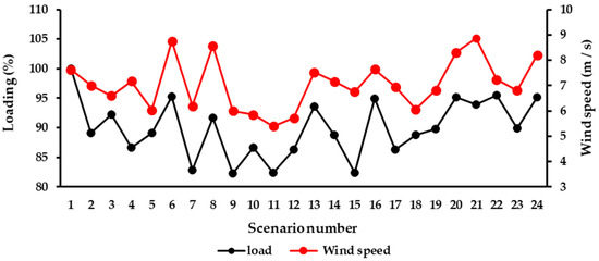
Figure 1.
Wind speed and load consumed over 24 scenarios.

Table 1.
Investment and operating factors of components used.
The Garver network is a benchmark system and is widely used for investigating the efficiency of TEP’s models. It has six buses, three-generation units, and five load buses [22], [32]. Bus 5 was suggested as a candidate position for new wind units, and buses 2, 5, and 6 were suggested for new ESSs. The network’s initial configuration is shown in Figure 2. New candidate routes are presented in dash lines.
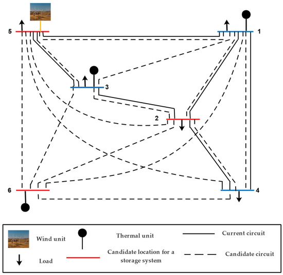
Figure 2.
The Garver network’s initial configuration.
The IEEE-24 bus system has 24 buses, eleven generation units, and seventeen load buses. Some modifications to the system were made in [32] to make congestions. The candidate locations for new wind units were buses 3, 10, and 19. While the candidate locations for ESSs were buses 2, 6, 8, 14, 20, 21, 22, and 24. The initial configuration of the system is depicted in Figure 3.
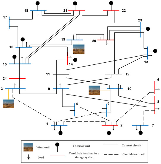
Figure 3.
The IEEE 24-bus system’s initial configuration.
4.2. Testing the Performance of SO-SCA
Figure 4, Figure 5, Figure 6 and Figure 7 show the convergence curves of the hybrid algorithm using the two approaches, SO and SCA, over ten runs. Noteworthy, all the simulations in this section were carried out without embedding L1 and L2 securities. The population size was 30 for SO-SCA #2 and 40 for SO-SCA #1, SO, and SCA. It is shown that the series approach effectively solved the Garver network in terms of standard deviation and quality of solutions compared to the parallel approach, as shown in Table 2. For the IEEE 24-bus system, SO-SCA #1 gave a lower standard deviation than SO-SCA #2, as illustrated in Table 3. Regarding SO and SCA, SCA achieved better performance than SO for the 24-bus system, but SO was superior to SCA in solving the Garver network.
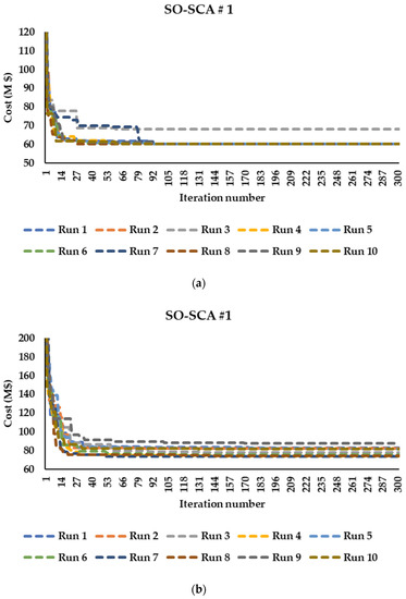
Figure 4.
Convergence curves of SO-SCA (first approach) over 10 runs: (a) Garver network and (b) The 24-bus system.
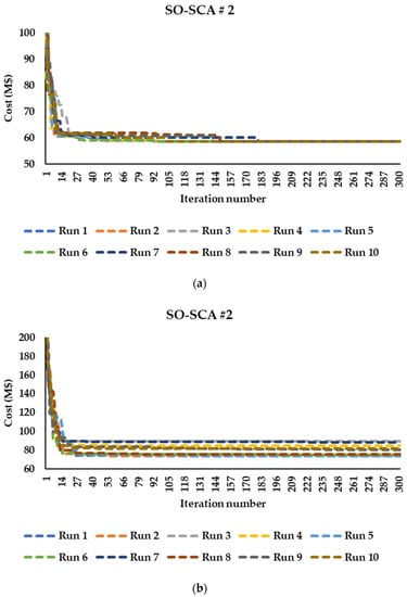
Figure 5.
Convergence curves of SO-SCA (second approach) over 10 runs: (a) Garver network and (b) The 24-bus system.
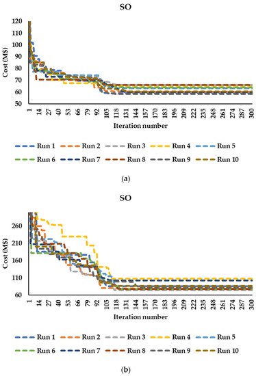
Figure 6.
Convergence curves of SO over ten runs: (a) Garver network and (b) The 24-bus system.
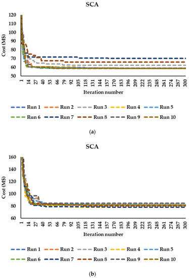
Figure 7.
Convergence curves of SCA over 10 runs: (a) Garver network and (b) The 24-bus system.
Table 2.
Simulation results of SO-SCA #1, SO-SCA #2, SO, and SCA for the Garver network.
Table 3.
Simulation results of SO-SCA #1, SO-SCA #2, SO, and SCA for the 24-bus system.
Table 2 and Table 3 explain that SCA converged faster than other algorithms. The time required by SCA to execute one run was about 144.18 s for the Garver network and 261.59 for the IEEE 24-bus system. While SO-SCA #1 ranked second in the convergence speed. It consumed 227.15 s to do one run on the Garver network and 348.81 s on the 24-bus system. SO-SCA #2 was the slowest. It needed 426.25 s to solve the Garver network and 551.45 s to solve the 24-bus system.
Based on all results, it can be concluded that the hybrid algorithm is efficient at solving TEP problems compared to the individual algorithms like SO and SCA. Both hybridization frameworks moved SO and SCA in each iteration to a better search area exploiting the best solution obtained by one of them. The results revealed that the series approach is recommended for solving small-scale systems, while the parallel process is preferred in solving larger systems.
4.3. Testing the Performance of SO-SCA-Based Load Forecasting Technique
The performance of SO-SCA-the based load forecasting technique was compared with PSO-, SCA-, SO, and least error squares (LES) estimation-based methods. The estimated parameters are given in Table 4 and Table 5. The predicted load using all algorithms is depicted in Figure 8.
Table 4.
The linear model estimated parameters based on different techniques.
Table 5.
The quadratic model estimated parameters based on different techniques.
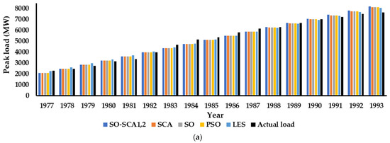
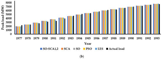
Figure 8.
Estimated load using SO-SCA-, SCA-, SO-, PSO- and LES-based techniques: (a) linear model, (b) quadratic model.
Table 4 and Table 5 show that SO-SCA#1 and SO-SCA#2 gave the least average error of 3.803074% for the linear model and 3.323598% for the quadratic model. The results also illustrated that SCA was superior to SO, PSO and LES in terms of average error. The linear model was 3.832615% for SCA, 3.8336% for SO, and 3.8336% and 4.2103 for PSO-and LES-based techniques. While for the quadratic model, it was 3.3375%, 3.3488%, 3.3488%, and 3.3873% for SCA-, SO-, PSO-, LES-based techniques.
The results demonstrated that the quadratic model was more suitable for fitting the testing data than the linear model because the minimum average error was 3.803074% for the linear model and 3.323598% for the quadratic model.
4.4. Testing Results of Garver Network
Table 6 details the results obtained using the proposed planning scheme. The results showed a significant change for projects required to achieve the L1 and L2 security constraints. The maximum number of circuits built in each route did not exceed 2 when the triggering event L2 was applied. In contrast, it did not surpass 3 for the triggering event L1. The total number of circuits installed was 7 for the event L1 and 10 for the event L2. The results emphasized that to achieve L1 security, there was a need for a new circuit at routes 3-5 and 5-6, two circuits at route 4-6, and three circuits at route 2-6. While meeting L2 security required new circuits at routes 2-3, 1-6, 3-4, 3-6, 4-6, and 5-6.
Table 6.
TEP’s projects for Garver network.
The results showed that the use of ESSs was essential to maintain power continuity and avoid cascading failures. The results indicated that NaS’s capacities required for the events L2 and L1 were 198.35 and 192.79, respectively. The best locations for the ESSs, to achieve L1 security were at nodes 2 and 5. Whilst the locations of ESSs needed to achieve L2 security were at buses 2, 5, and 6.
Figure 9 shows the short circuit current at scenario number24 as an example to verify that it did not exceed the maximum limit (6.5 p.u) and that the short-circuit constraints were achieved in each scenario. It is worth mentioning that the total size of FCLs required ranged between 0.59 + 5.9i p.u and 1.24 + 12.4i p.u. The results also illustrated that the buses’ voltage did not violate their limits (0.9–1.1 p.u). Figure 10 points to the voltage at each bus for scenario number 24 as an example.
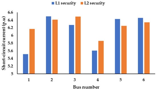
Figure 9.
Short-circuit current at scenario number 24 for the Garver system.
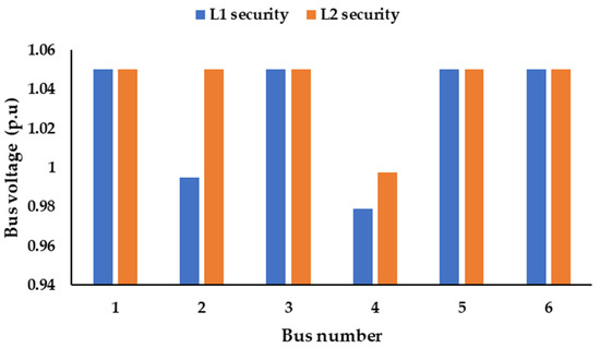
Figure 10.
Buses’ voltage at scenario number 24 for the Garver system.
The previous results imply that the triggering event L2 was the worst, and the probability of occurring complete blackouts was high. The cost of projects needed for fulfilling L2 security exceeded 17.41 % compared to the cost of L1 projects.
4.5. Testing Results of the IEEE 24-Bus System
Similar to the Garver network, simulations on the 24-bus system confirmed the gravity of the L2 event compared to the L1 event. This is clearly shown in the size of ESSs required and the planning cost. There was an increase of about 108% in the size of ESSs to meet L2 security. The results pointed to the size of NaS batteries required for ensuring L1 security was MWh 29.43 at bus 6. Whilst 60.123 and 1.172 MWh of NaS batteries at buses 6 and 21 were needed to fulfil L2 security.
According to Table 7, new circuits were installed at the routes 1-2, 1-3, 2-4, 2-6, 7-2, 7-5, and 7-8 to guarantee L1 and L2 securities. It is worth emphasizing that the reliance on the location of new circuits was not enough to achieve the short circuit-current constraints. The use of FCLs was necessary. The short-circuit current at scenario number 24, as an example, is depicted in Figure 11. The results indicated that the planning model was able to maintain the buses’ voltage within their limits. They did not violate the upper and lower bounds (0.9–1.1 p.u), as shown in Figure 12.
Table 7.
TEP’s projects for the 24-bus system.
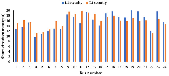
Figure 11.
Short-circuit current at scenario number 24 for the 24-bus system.
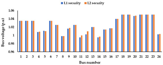
Figure 12.
Buses’ voltage at scenario number 24 for the 24-bus system.
Based on all previous findings, it can be concluded that relying on a single strategy to avoid the cascading failures of the electrical networks does not guarantee their security and resilience. Two simple strategies were applied in this work, which significantly affected the size and number of projects required and hence the cost. For the Garver network, the impact was clearly shown in the number and the location of new circuits. While for the 24-bus system, the size of ESSs was affected by the type of cascading failures
The TEP problem is complex, and the hybrid of two meta-heuristic algorithms effectively solved TEP models compared to individual algorithms. The two hybridization frameworks were superior in terms of standard deviation and quality of solutions. Further, the hybrid algorithm was more accurate in forecasting the electrical loads in the long term than some methods introduced in the literature.
5. Conclusions
In this work, a resilience TEP model was suggested to ensure networks’ reliability and supply the future electrical demands. The short-circuit current and the cascading failure constraints were considered to achieve the resilience requirements. NaSs and FCLs’ planning models were incorporated into the proposed TEP model to achieve these targets. Two simple scanning matrices, L1 and L2, were modeled as triggering events for cascading failures. L1 simulated a power system under a single circuit’s outage between two nodes. L2 focused on the outage of all circuits between two nodes as the triggering event for cascading failures. The results showed that simulating a single strategy for cascading failures of power systems does not guarantee their security and resilience. The triggering event L2 was the worst. The probability of occurring complete blackouts was high. The impact was clearly shown in the number and the location of new circuits for the Garver network, while it affected the size of ESSs installed for the IEEE 24-bus system.
The proposed TEP problem was a large-scale non-linear optimization problem, and a hybrid of two meta-heuristic techniques, namely SO and SCA, was adopted. Two hybridization approaches were applied to enhance the exploration and exploitation stages. SO and SCA operated parallel in the first approach to calculate new variables in each iteration. While in the second approach, SO and SCA operated in a series mechanism. The results revealed that the second approach effectively solved small-scale systems, whereas the first approach efficiently solved larger systems.
Further, the results proved that both approaches were superior in terms of standard deviation and quality of solutions compared to individual algorithms. A long-term load forecasting technique based on SO-SCA was proposed. It was shown that the suggested method gave accurate results compared to PSO, SO, SCA, and LES.
This work is only concerned with investigating two simple cascading failure events, but more events that pose a greater threat to the network should be considered to get a secure network. More studies are required to evaluate the impact of including the transient stability constraints on enhancing power systems’ securities and resilience. In addition, the planning model needs to be extended to study the effects of the optimal mix of transmission lines, distributed generators, FCLs, ESSs, reactive source compensators, demand response, and thyristor-controlled series compensators on improving power systems’ securities and avoiding cascading failures. The performance of the hybrid SO-SCA should also be tested on larger systems with an extensive search space.
Funding
This project is funding under the grant no. (G: 702-135-1443).
Institutional Review Board Statement
Not applicable.
Informed Consent Statement
Not applicable.
Data Availability Statement
The data presented in this study are available on request from the corresponding author. The data are not publicly available due to their large size.
Acknowledgments
The author acknowledges the Deanship of Scientific Research (DSR) at King Abdulaziz University, Jeddah, Saudi Arabia, for funding this project, under grant no. (G: 702-135-1443). The Author also acknowledges the support provided by King Abdullah City for Atomic and Renewable Energy (K.A.CARE) under K.A.CARE-King Abdulaziz University Collaboration Program.
Conflicts of Interest
The author declares no conflict of interest.
Nomenclature
| ESS | Energy storage system |
| FCL | Fault current limiter |
| SCA | Sine cosine algorithm |
| SO | Snake optimizer |
| SO-SCA #1 | The hybrid of SO and SCA using the first approach |
| SO-SCA #2 | The hybrid of SO and SCA using the second approach |
| SOC | State of charge |
| NaS | Sodium-Sulfur batteries |
| RESs | Renewable and sustainable energy sources |
| TCSCs | Thyristor-controlled series compensators |
| TEP | Transmission expansion planning |
| Input Data and Indices | |
| Conductance and susceptance of the route between bus i and j | |
| Cost of circuits installed between bus i and bus j | |
| Cost of FCL installed | |
| Capital cost of NaS built | |
| Operating cost of NaS | |
| Capital cost of new generation unit built | |
| Operating cost of generation units | |
| Maximum number of scenarios | |
| Number of batteries installed at scenario h, and maximum number of batteries can be installed at bus i | |
| Number of generation units at bus i and scenario h | |
| Power produced from the generation units in MW | |
| Output active power in MW of thermal unit and RSES at scenario h, respectively | |
| Active power consumed by the load at bus i (MW) | |
| Charging and discharging power of an ESS at bus i (MW) | |
| Rated power of the selected ESS | |
| Output reactive power in MVAR of thermal unit at scenario h | |
| Reactive power consumed by the load at bus i (MVAR) | |
| Apparent power flow in a route between bus i and j in both terminals (MVA) | |
| maximum rated of power flow in a route between bus i and j (MVA) | |
| SOC of ESS at bus i and scenario h | |
| Voltage magnitude and angle at bus i (p.u) | |
| Charging and discharging efficiencies of ESS | |
| λ, y | Discount rate and the lifetime of the project |
| Size of FCL installed in the route i-j | |
References
- Mutlu, S.; Şenyiğit, E. Literature review of transmission expansion planning problem test systems: Detailed analysis of IEEE-24. Electr. Power Syst. Res. 2021, 201, 107543. [Google Scholar] [CrossRef]
- Mahdavi, M.; Sabillon Antunez, C.; Ajalli, M.; Romero, R. Transmission Expansion Planning: Literature Review and Classification. IEEE Syst. J. 2019, 13, 3129–3140. [Google Scholar] [CrossRef]
- Hamidpour, H.; Aghaei, J.; Pirouzi, S.; Dehghan, S.; Niknam, T. Flexible, reliable, and renewable power system resource expansion planning considering energy storage systems and demand response programs. IET Renew. Power Gener. 2019, 13, 1862–1872. [Google Scholar] [CrossRef]
- Esmaili, M.; Ghamsari-Yazdel, M.; Amjady, N.; Chung, C.Y.; Conejo, A.J. Transmission Expansion Planning including TCSCs and SFCLs: A MINLP Approach. IEEE Trans. Power Syst. 2020, 35, 4396–4407. [Google Scholar] [CrossRef]
- Franken, M.; Barrios, H.; Schrief, A.B.; Moser, A. Transmission expansion planning via power flow controlling technologies. IET Gener. Transm. Distrib. 2020, 14, 3530–3538. [Google Scholar] [CrossRef]
- Moradi-Sepahvand, M.; Amraee, T. Hybrid AC/DC Transmission Expansion Planning Considering HVAC to HVDC Conversion under Renewable Penetration. IEEE Trans. Power Syst. 2021, 36, 579–591. [Google Scholar] [CrossRef]
- Refaat, M.M.; Aleem, S.H.E.; Atia, Y.; Ali, Z.M.; El-Shahat, A.; Sayed, M.M. A Mathematical Approach to Simultaneously Plan Generation and Transmission Expansion Based on Fault Current Limiters and Reliability Constraints. Mathematics 2021, 9, 2771. [Google Scholar] [CrossRef]
- Abdi, H.; Moradi, M.; Lumbreras, S. Metaheuristics and Transmission Expansion Planning: A Comparative Case Study. Energies 2021, 14, 3618. [Google Scholar] [CrossRef]
- Abbasi, S.; Abdi, H.; Bruno, S.; La, M. Transmission network expansion planning considering load correlation using unscented transformation. Electr. Power Energy Syst. 2018, 103, 12–20. [Google Scholar] [CrossRef]
- Ramachandran, M.; Mirjalili, S.; Nazari-Heris, M.; Parvathysankar, D.S.; Sundaram, A.; Charles Gnanakkan, C.A.R. A hybrid Grasshopper Optimization Algorithm and Harris Hawks Optimizer for Combined Heat and Power Economic Dispatch problem. Eng. Appl. Artif. Intell. 2022, 111, 104753. [Google Scholar] [CrossRef]
- Cetinbas, I.; Tamyurek, B.; Demirtas, M. The Hybrid Harris Hawks Optimizer-Arithmetic Optimization Algorithm: A New Hybrid Algorithm for Sizing Optimization and Design of Microgrids. IEEE Access 2022, 10, 19254–19283. [Google Scholar] [CrossRef]
- Almalaq, A.; Alqunun, K.; Refaat, M.M.; Farah, A.; Benabdallah, F.; Ali, Z.M.; Aleem, S.H.E.A. Towards Increasing Hosting Capacity of Modern Power Systems through Generation and Transmission Expansion Planning. Sustainability 2022, 14, 2998. [Google Scholar] [CrossRef]
- Sousa, A.S.; Asada, E.N. Combined heuristic with fuzzy system to transmission system expansion planning. Electr. Power Syst. Res. 2011, 81, 123–128. [Google Scholar] [CrossRef]
- Armaghani, S.; Hesami Naghshbandy, A.; Shahrtash, S.M. A novel multi-stage adaptive transmission network expansion planning to countermeasure cascading failure occurrence. Int. J. Electr. Power Energy Syst. 2020, 115, 105415. [Google Scholar] [CrossRef]
- Mehrtash, M.; Kargarian, A. Risk-based dynamic generation and transmission expansion planning with propagating effects of contingencies. Int. J. Electr. Power Energy Syst. 2020, 118, 105762. [Google Scholar] [CrossRef]
- Qorbani, M.; Amraee, T. Long term transmission expansion planning to improve power system resilience against cascading outages. Electr. Power Syst. Res. 2021, 192, 106972. [Google Scholar] [CrossRef]
- Gjorgiev, B.; David, A.E.; Sansavini, G. Cascade-risk-informed transmission expansion planning of AC electric power systems. Electr. Power Syst. Res. 2022, 204, 107685. [Google Scholar] [CrossRef]
- Peng, L.; Liu, S.; Liu, R.; Wang, L. Effective long short-term memory with differential evolution algorithm for electricity price prediction. Energy 2018, 162, 1301–1314. [Google Scholar] [CrossRef]
- Neshat, M.; Nezhad, M.M.; Abbasnejad, E.; Mirjalili, S.; Groppi, D.; Heydari, A.; Tjernberg, L.B.; Astiaso Garcia, D.; Alexander, B.; Shi, Q.; et al. Wind turbine power output prediction using a new hybrid neuro-evolutionary method. Energy 2021, 229, 120617. [Google Scholar] [CrossRef]
- Xie, Y.; Li, C.; Tang, G.; Liu, F. A novel deep interval prediction model with adaptive interval construction strategy and automatic hyperparameter tuning for wind speed forecasting. Energy 2021, 216, 119179. [Google Scholar] [CrossRef]
- AlRashidi, M.R.; EL-Naggar, K.M. Long term electric load forecasting based on particle swarm optimization. Appl. Energy 2010, 87, 320–326. [Google Scholar] [CrossRef]
- Fathy, A.A.; Elbages, M.S.; El-Sehiemy, R.A.; Bendary, F.M. Static transmission expansion planning for realistic networks in Egypt. Electr. Power Syst. Res. 2017, 151, 404–418. [Google Scholar] [CrossRef]
- Refaat, M.M.; Aleem, S.H.E.A.; Atia, Y.; Ali, Z.M.; Sayed, M.M. Multi-stage dynamic transmission network expansion planning using lshade-spacma. Appl. Sci. 2021, 11, 2155. [Google Scholar] [CrossRef]
- Hong, W.-C. Forecasting electric load by support vector machines with genetic algorithms. J. Adv. Comput. Intell. Intell. Inform. 2005, 9, 134–141. [Google Scholar]
- Hashim, F.A.; Hussien, A.G. Snake Optimizer: A novel meta-heuristic optimization algorithm. Knowl.-Based Syst. 2022, 242, 108320. [Google Scholar] [CrossRef]
- Mirjalili, S. SCA: A Sine Cosine Algorithm for solving optimization problems. Knowl.-Based Syst. 2016, 96, 120–133. [Google Scholar] [CrossRef]
- Dagoumas, A.S.; Koltsaklis, N.E. Review of models for integrating renewable energy in the generation expansion planning. Appl. Energy 2019, 242, 1573–1587. [Google Scholar] [CrossRef]
- Naderi, E.; Pourakbari-Kasmaei, M.; Lehtonen, M. Transmission expansion planning integrated with wind farms: A review, comparative study, and a novel profound search approach. Int. J. Electr. Power Energy Syst. 2020, 115, 105460. [Google Scholar] [CrossRef]
- Mostafa, M.H.; Abdel Aleem, S.H.E.; Ali, S.G.; Ali, Z.M.; Abdelaziz, A.Y. Techno-economic assessment of energy storage systems using annualized life cycle cost of storage (LCCOS) and levelized cost of energy (LCOE) metrics. J. Energy Storage 2020, 29, 101345. [Google Scholar] [CrossRef]
- Refaat, M.M.; Aleem, S.H.E.A.; Atia, Y.; Ali, Z.M.; Sayed, M.M. AC and DC Transmission Line Expansion Planning Using Coronavirus Herd Immunity Optimizer. In Proceedings of the 2021 22nd International Middle East Power Systems Conference (MEPCON), Assiut, Egypt, 14–16 December 2021; pp. 313–318. [Google Scholar]
- Saboori, H.; Hemmati, R. Considering carbon capture and storage in electricity generation expansion planning. IEEE Trans. Sustain. Energy 2016, 7, 1371–1378. [Google Scholar] [CrossRef]
- Zhang, H.; Heydt, G.T.; Vittal, V.; Mittelmann, H.D. Transmission expansion planning using an AC model: Formulations and possible relaxations. In Proceedings of the 2012 IEEE Power and Energy Society General Meeting, San Diego, CA, USA, 22–26 July 2012; pp. 1–8. [Google Scholar]
Publisher’s Note: MDPI stays neutral with regard to jurisdictional claims in published maps and institutional affiliations. |
© 2022 by the author. Licensee MDPI, Basel, Switzerland. This article is an open access article distributed under the terms and conditions of the Creative Commons Attribution (CC BY) license (https://creativecommons.org/licenses/by/4.0/).