
Robust Parametric Identification for ARMAX Models with Non-Gaussian and Coloured Noise: A Survey


Abstract
1. Introduction
1.1. Road Map of This Survey
- −
- Review of publications:
- It contains the descriptions of the important survey published in the 1970’s–1990’s (Åström, Becky, Ljung and Gunnarson, Billings among others).
- Nongaussian noises have been studied by Huber, Tsypkin and Polyak.
- −
- Problem formulation and model description:
- The ARMAX model with correlated non-Gaussian noise, generated by a stable and non-minimal phase filter, is introduced.
- −
- Some classes of noise p.d.f.:
- In a rigorous mathematical manner several classes of random stationary sequences with different p.d.f. as an input of a forming filter are considered (all symmetric distributions non-singular in origin, all symmetric distributions with a bounded variance, all symmetric “approximately normal” distributions and “approximately uniform” distributions).
- −
- Main assumptions:
- These concern the martingale difference property with conditional bounder second moment for stochastic sequences in the input of the forming filter, stability and minimal-phase property for this filter, independent of this sequence with other measurable inputs).
- −
- Regression representation format:
- The extended regression form of the considered model is introduced.
- −
- Main contribution of the paper:
- The exact presentation of the main contribution of the paper.
- −
- Why LSM does not work for the identification of ARMAX models with correlated noise:
- A simple example exhibiting the lack of workability of this technique in the case of dynamic (autoregression) models is described in detail for a reader who is not actively involved in the least-squares method.
- −
- Some other identification techniques:
- Identification of non-stationary parameters and the Bayesian method, matrix forgetting factor and its adaptive version are reviewed.
- −
- Regular observations and information inequality for observations with coloured noise:
- the Cramér–Rao bound (CRB) and the Fisher information, characterising the maximal possible rate of estimation under the given information resource, are presented.
- −
- Robust version of the maximum likelihood method with whitening (MLMW procedure):
- This approach is demonstrated to reach the CRB bound, indicating that it is asymptotically the best among all identification procedures.
- −
- Recurrent identification procedures with nonlinear residual transformations: static (regression) and dynamic (autoregression) models:
- Within a specified noise p.d.f. class, it is proven that such a strategy with particular selection of nonlinear residual transformation is resilient (robust) optimum in achieving min–max error variance in CRB inequality.
- −
- Instrumental variables ethod (IVM):
- IV or total least-squares estimators is the method which also recommends to estimate parameters in the presence of coloured noises with a finite correlation.
- −
- Joint parametric identification of ARMAX model and the forming filter:
- The “generalised residual sequence” is introduced, which is shown to be asymptotically closed to the independent sequence acting in the input of the forming filter, which helps to resolve the identification problem in an extended parametric space.
- Numerical example.
- Discussion and conclusions.
- −
- Appendix A and abbreviations:
- This part offers proofs of some of the article’s claims that appear to be significant from the authors’ perspective, as well as a list of acronyms used throughout the work.
1.2. Review of the System Identification Literature
1.3. Classical Surveys on Identification
1.4. Identification under Correlated Noise Perturbations
1.5. Identification of ARMAX and NARMAX Models
2. Problem Formulation
2.1. Robust Parametric Identification Model Description
- is scalar sequence of available on-line state variables.
- is a measurable input sequence (deterministic or, in general, stochastic).
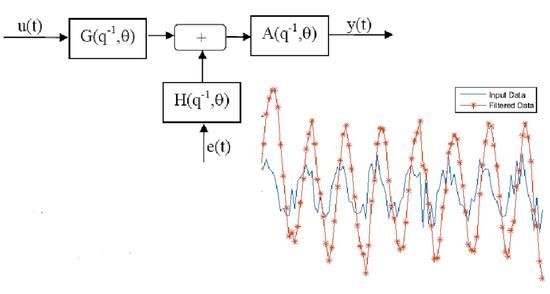
- is a noise sequence (not available during the process) generated by the exogenous systemwhich can be symbolically represented as the forming filterwith the transition function
- as an independent zero mean stationary sequence with the probability density function (p.d.f.) which may be unknown but belonging to some given class of p.d.f., that is,
2.2. Some Classes of p.d.f.
- Class (of all symmetric distributions non singular in the point ):We deal with this class if there is not any a priori information on a noise distribution .
- Class (of all symmetric distributions with a bounded variance):
- Class (of all symmetric “approximately normal” distributions):where is the centred Gaussian distribution density with the variance defined by and is another distribution density. The parameter characterises the level of the effect of a “dirty” distribution to the basic Gaussian distribution .
- Class (of all symmetric “approximately uniform” distributions):whereis the centred uniform distribution and is one process with a different distribution density. The parameter characterises the level of the effect of a “dirty” distribution to the basic one .
2.3. Main Assumptions
- All random variables are defined on the probability space with the -algebras flow
- For all n
- The measurable input sequence is of bounded power:and is independent of i.e.,
- It is assumed that the forming filter is stable and “minimal-phase”, that is, both polynomials and are Hurwitz, i.e., have all roots inside of the unite circle in the complex plain.
- The ARMAX plant (1) is stable: the polynomialis Hurwitz.
2.4. Regression Format Representation
2.5. Robust Parametric Identification Problem Formulation
- −
- the parameters of the forming filter are known.
- −
- The parameters of the forming filter are also unknown.
2.6. Main Contribution of the Paper
- The Cramer–Rao information bound for ARMAX (autoregression moving average models with exogenous inputs) under non-Gaussian noises is derived.
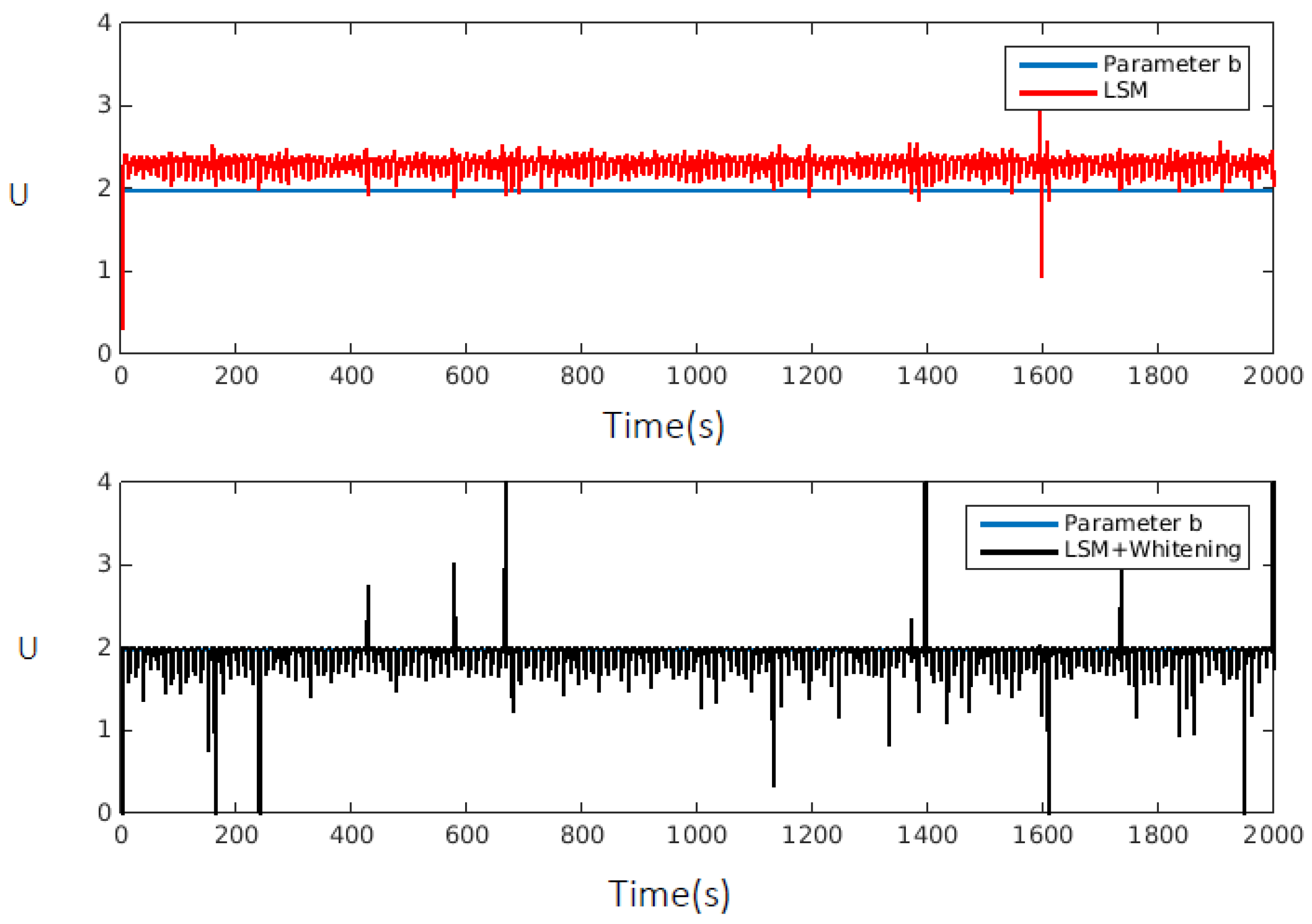
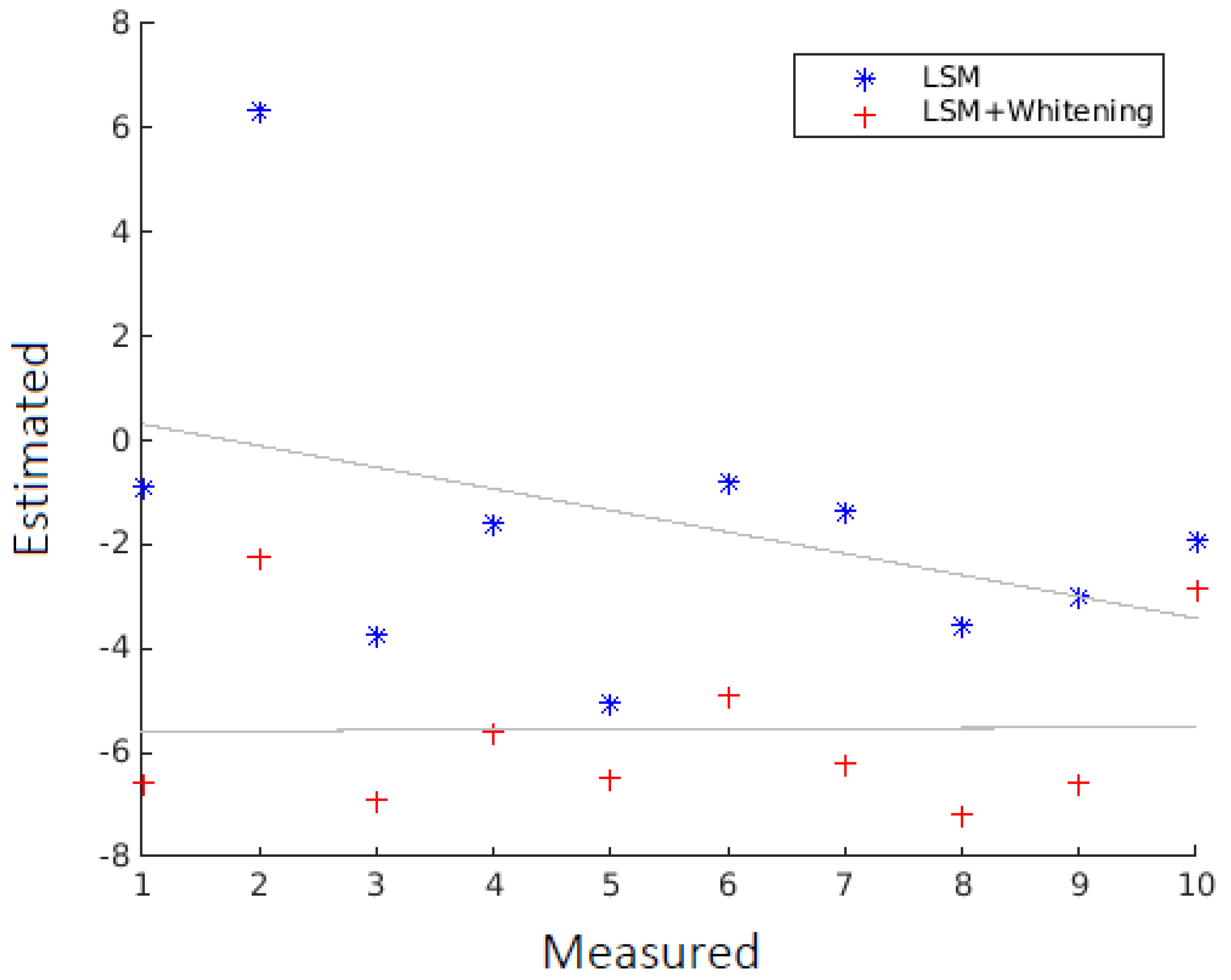
- It is shown that the direct implementation of the least-squares method (LSM) leads to an incorrect (shifted) parameter estimation.
- This inconsistency can be corrected by the implementation of the parallel use of the MLMW (maximum likelihood method with whitening) procedure, applied to all measurable variables of the model, and a nonlinear residual transformation using the information on the distribution density of a non-Gaussian noise, participating in moving average structure.
- The design of the corresponding parameter estimator, realising the suggested MLMW procedure, containing a parallel on-line “whitening” process as well as a nonlinear residual transformation, is presented in detail.
- It is shown that the MLMW procedure attains the obtained information bound, and hence, is asymptotically optimal.
3. Why LSM Does Not Work for the Identification of ARMAX Models with Correlated Noise
4. Some Other Identification Techniques
Identification of Non-Stationary Parameters and Bayesian Method
5. Regular Observations and Information Inequality for Observations with Coloured Noise
5.1. Main Definitions and the Cramer–Rao Information Inequality
- −
- If then the estimate is called unbiased and asymptotically unbiased if .
- −
- The observations are referred to be as regular on the class C of parameters ifand for any
- −
- The matrix is called the Fisher information matrix for the set of available observations .
5.2. Fisher Information Matrix Calculation
5.3. Asymptotic Cramer–Rao Inequality
5.4. Whitening Process for Stable and Minimal-Phase Forming Filters
5.5. Cramer–Rao Inequality for ARMAX Models with a Generating Noise from the Class of p.d.f.
6. Robust Version of Maximum Likelihood Method with Whitening: MLMW Procedure
6.1. Whitening Method and Its Application
6.2. Recurrent Robust Identification Procedures with Whitening and a Nonlinear Residual Transformation
- 1.
- is i.i.d. sequence with
- 2.
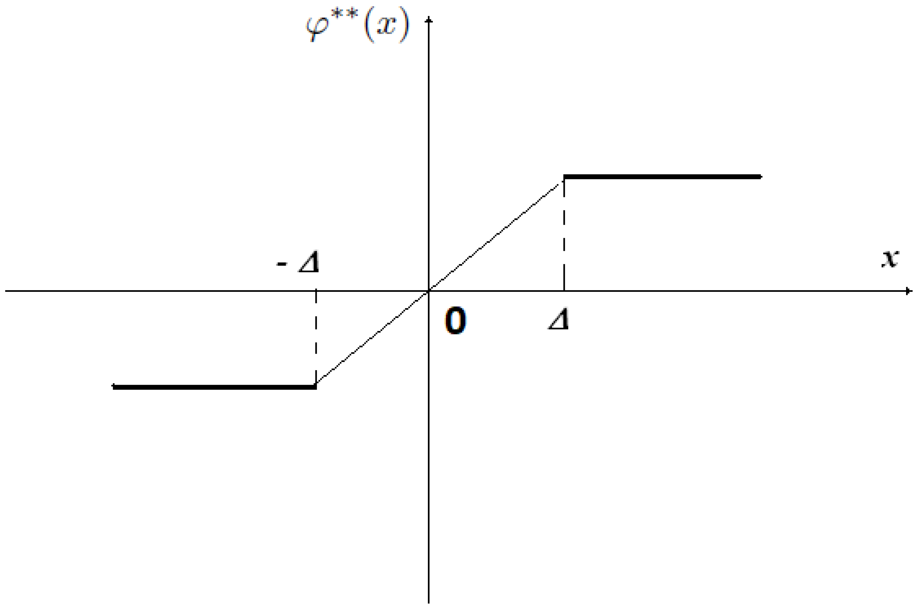
- The nonlinear transformation satisfies the conditionswiththen
- −
- The distribution is the “worst” within the class .
- −
- The nonlinear transformation is “the best one” oriented on the “worst” noise with the distribution .
6.3. Particular Cases for Static (Regression) Models
6.4. Robust Identification of Dynamic ARX Models
- (1)
- Class (containing among others the Gaussian distribution ).
- (2)
- Class (containing all centred distributions with a variance not less than a given value):
7. Instrumental Variables Method for ARMAX Model with Finite Noise Correlation
7.1. About IVM
7.2. Instrumental Variables and the System of Normal Equations
- (1)
- (2)
- then the estimate is asymptotically consistent with probability 1, namely, .
8. Joint Parametric Identification of ARMAX Model and the Forming Filter
8.1. An Equivalent ARMAX Representation
8.2. Auxiliary Residual Sequence
8.3. Identification Procedure
8.4. Recuperation of the Model Parameters from the Obtained Current Estimates
8.4.1. Special Case When the Recuperation Process Can Be Realised Directly
8.4.2. General Case Requiring the Application of Gradient Descent Method (GDM)
9. Numerical Example
Raised Cosine Distribution
10. Discussion
- −
- Instrumental variables method (IVM) for ARMAX models with a finite noise-correlation.
- −
- The nonlinear residual transformation method for simultaneous parametric identification of the ARMAX model and the forming filter.Both techniques are not asymptotically effective, as they do not achieve the Cramer–Rao information limits.
11. Conclusions
Author Contributions
Funding
Institutional Review Board Statement
Informed Consent Statement
Data Availability Statement
Conflicts of Interest
Abbreviations
| ARX | Autoregressive model with exogenous variables |
| ARMAX | Autoregression moving average exogenous input |
| NARMAX | Nonlinear autoregression moving average exogenous input |
| LSM | Least-squares method |
| IVM | Instrumental variables method |
| LNL | Large number law |
| NARMAX | Nonlinear autoregressive moving average with |
| CRB | Cramer–Rao bound |
| FIM | Fisher information |
| MVU | Minimum variance unbiased |
| MLMW | Maximum likelihood method with whitening |
| DWM | Direct whitening method |
| WECC | Western Electricity Coordinating Council |
| KARMAX | Autoregressive moving average explanatory input model of the Koyck kind |
| IVAML | Instrumental variable approximate maximum likelihood |
| RIV | Refinen instrumental variables |
| GDM | Gradient descent method |
Appendix A
Appendix A.1. Proof of Lemma 2
- By the Cauchy–Schwarz inequalityvalid for any p.d.f. and any noise density distribution (for which the integrals have a sense), for after integrating by parts it followswhere the equality is attained when is any constant. Taking in (A2) and using the identity leads towhere the equality is attained when or equivalently, for With we haveSo, and the worst noise distribution within is (55).
Appendix A.2. Proof of Lemma 3
Appendix A.3. Proof of Lemma 4
- For we haveimplyingSo, the worst noise distribution within is .
Appendix A.4. Proof of Lemma 5
- (without details). From (7) it followsSo, we need to solve the following variational problem:
References
- Bender, E. An Introduction to Mathematical Modeling; Dover Publications, Inc.: Mineola, NY, USA, 2012. [Google Scholar]
- Hugues, G.; Liuping, W. Identification of Continuous-Time Models from Sampled Data; Springer: Berlin/Heidelberg, Germany, 2008. [Google Scholar]
- Åström, K.J.; Eykhoff, P. System identification—A survey. Automatica 1971, 7, 123–162. [Google Scholar] [CrossRef]
- Bekey, G.A. System Identification—An Introduction and a Survey. Simulation 1970, 15, 151–166. [Google Scholar] [CrossRef]
- Ljung, L.; Gunnarsson, S. Adaptation and tracking in system identification—A survey. Automatica 1990, 26, 7–21. [Google Scholar] [CrossRef]
- Billings, S.A. Identification of Nonlinear Systems—A Survey. In Proceedings of the IEE Proceedings D-Control Theory and Applications; IET: London, UK, 1980; Volume 127, pp. 272–285. [Google Scholar]
- Ljung, L. Perspectives on system identification. Annu. Rev. Control 2010, 34, 1–12. [Google Scholar] [CrossRef]
- Ljung, L.; Chen, T.; Mu, B. A shift in paradigm for system identification. Int. J. Control 2020, 93, 173–180. [Google Scholar] [CrossRef]
- Tudor, C. Procesos Estocásticos; Sociedad Mexicana de Matemáticas: Ciudad de Mexico, Mexico, 1994. [Google Scholar]
- Sobczyk, K. Stochastic Differential Equations: With Applications to Physics and Engineering; Springer Science and Business Media: Berlin/Heidelberg, Germany, 2013. [Google Scholar]
- Feng, D.; Liu, P.X.; Liu, G. Auxiliary model based multi-innovation extended stochastic gradient parameter estimation with colored measurement noises. Signal Process. 2009, 89, 1883–1890. [Google Scholar]
- Vo, B.-N.; Antonio Cantoni, K.L.T. Filter Design with Time Domain Mask Constraints: Theory and Applications; Springer Science and Business Media: Berlin/Heidelberg, Germany, 2013; Volume 56. [Google Scholar]
- Huber, P. Robustness and Designs: In “A Survey of Statistical Design and Linear Models”; North-Holland Publishing Company: Amsterdam, The Netherlands, 1975. [Google Scholar]
- Tsypkin, Y.; Polyak, B. Robust likelihood method. Dyn. Syst. Math. Methods Oscil. Theory Gor’Kii State Univ. 1977, 12, 22–46. (In Russian) [Google Scholar]
- Poznyak, A.S. Robust identification under correlated and non-Gaussian noises: WMLLM procedure. Autom. Remote Control 2019, 80, 1628–1644. [Google Scholar] [CrossRef]
- Mokhlis, S.E.; Sadki, S.; Bensassi, B. System identification of a dc servo motor using arx and armax models. In Proceedings of the 2019 International Conference on Systems of Collaboration Big Data, Internet of Things & Security (SysCoBIoTS), Granada, Spain, 22–25 October 2019; IEEE: Piscataway, NJ, USA, 2019; pp. 1–4. [Google Scholar]
- AldemĠR, A.; Hapoğlu, H. Comparison of ARMAX Model Identification Results Based on Least Squares Method. Int. J. Mod. Trends Eng. Res. 2015, 2, 27–35. [Google Scholar]
- Likothanassis, S.; Demiris, E. Armax model identification with unknown process order and time-varying parameters. In Signal Analysis and Prediction; Springer: Berlin/Heidelberg, Germany, 1998; pp. 175–184. [Google Scholar]
- Norton, J. Identification of parameter bounds for ARMAX models from records with bounded noise. Int. J. Control 1987, 45, 375–390. [Google Scholar] [CrossRef]
- Stoffer, D.S. Estimation and identification of space-time ARMAX models in the presence of missing data. J. Am. Stat. Assoc. 1986, 81, 762–772. [Google Scholar] [CrossRef]
- Mei, L.; Li, H.; Zhou, Y.; Wang, W.; Xing, F. Substructural damage detection in shear structures via ARMAX model and optimal subpattern assignment distance. Eng. Struct. 2019, 191, 625–639. [Google Scholar] [CrossRef]
- Ferkl, L.; Širokỳ, J. Ceiling radiant cooling: Comparison of ARMAX and subspace identification modelling methods. Build. Environ. 2010, 45, 205–212. [Google Scholar] [CrossRef]
- Rahmat, M.; Salim, S.N.S.; Sunar, N.; Faudzi, A.M.; Ismail, Z.H.; Huda, K. Identification and non-linear control strategy for industrial pneumatic actuator. Int. J. Phys. Sci. 2012, 7, 2565–2579. [Google Scholar] [CrossRef]
- González, J.P.; San Roque, A.M.S.M.; Perez, E.A. Forecasting functional time series with a new Hilbertian ARMAX model: Application to electricity price forecasting. IEEE Trans. Power Syst. 2017, 33, 545–556. [Google Scholar] [CrossRef]
- Wu, S.; Sun, J.Q. A physics-based linear parametric model of room temperature in office buildings. Build. Environ. 2012, 50, 1–9. [Google Scholar] [CrossRef]
- Jing, S. Identification of an ARMAX model based on a momentum-accelerated multi-error stochastic information gradient algorithm. In Proceedings of the 2021 IEEE 10th Data Driven Control and Learning Systems Conference (DDCLS), Suzhou, China, 14–16 May 2021; IEEE: Piscataway, NJ, USA, 2021; pp. 1274–1278. [Google Scholar]
- Le, Y.; Hui, G. Optimal Estimation for ARMAX Processes with Noisy Output. In Proceedings of the 2020 Chinese Automation Congress (CAC), Shanghai, China, 6–8 November 2020; IEEE: Piscataway, NJ, USA, 2020; pp. 5048–5051. [Google Scholar]
- Correa Martinez, J.; Poznyak, A. Switching Structure Robust State and Parameter Estimator for MIMO Nonlinear Systems. Int. J. Control 2001, 74, 175–189. [Google Scholar] [CrossRef]
- Shieh, L.; Bao, Y.; Chang, F. State-space self-tuning controllers for general multivariable stochastic systems. In Proceedings of the 1987 American Control Conference, Minneapolis, MN, USA, 10–12 June 1987; IEEE: Piscataway, NJ, USA, 1987; pp. 1280–1285. [Google Scholar]
- Correa-MartÍnez, J.; Poznyak, A.S. Three electromechanical examples of robust switching structure state and parameter estimation. In Proceedings of the 38th IEEE Conference on Decision and Control, Phoenix, AZ, USA, 7–10 December 1999; pp. 3962–3963. [Google Scholar] [CrossRef]
- Mazaheri, A.; Mansouri, M.; Shooredeli, M. Parameter estimation of Hammerstein-Wiener ARMAX systems using unscented Kalman filter. In Proceedings of the 2014 Second RSI/ISM International Conference on Robotics and Mechatronics (ICRoM), Tehran, Iran, 15–17 October 2014; IEEE: Piscataway, NJ, USA, 2014; pp. 298–303. [Google Scholar]
- Tsai, J.S.-H.; Hsu, W.; Lin, L.; Guo, S.; Tann, J.W. A modified NARMAX model-based self-tuner with fault tolerance for unknown nonlinear stochastic hybrid systems with an input—Output direct feed-through term. ISA Trans. 2014, 53, 56–75. [Google Scholar] [CrossRef]
- Pu, Y.; Chen, J. A novel maximum likelihood-based stochastic gradient algorithm for Hammerstein nonlinear systems with coloured noise. Int. J. Model. Identif. Control 2019, 32, 23–29. [Google Scholar] [CrossRef]
- Wang, D.; Fan, Q.; Ma, Y. An interactive maximum likelihood estimation method for multivariable Hammerstein systems. J. Frankl. Inst. 2020, 357, 12986–13005. [Google Scholar] [CrossRef]
- Zheng, W.X. On least-squares identification of ARMAX models. IFAC Proc. Vol. 2002, 35, 391–396. [Google Scholar] [CrossRef]
- Poznyak, A.S. Advanced Mathematical Tools for Automatic Control Engineers Volume 2: Stochastic Techniques; Elsevier: Amsterdam, The Netherlands, 2009. [Google Scholar]
- Medel-Juárez, J.; Poznyak, A.S. Identification of Non Stationary ARMA Models Based on Matrix Forgetting. 1999. Available online: http://repositoriodigital.ipn.mx/handle/123456789/15474 (accessed on 6 February 2022).
- Poznyak, A.; Medel, J. Matrix Forgetting with Adaptation. Int. J. Syst. Sci. 1999, 30, 865–878. [Google Scholar] [CrossRef]
- Cerone, V. Parameter bounds for armax models from records with bounded errors in variables. Int. J. Control 1993, 57, 225–235. [Google Scholar] [CrossRef]
- He, L.; Kárnỳ, M. Estimation and prediction with ARMMAX model: A mixture of ARMAX models with common ARX part. Int. J. Adapt. Control Signal Process. 2003, 17, 265–283. [Google Scholar] [CrossRef]
- Yin, L.; Gao, H. Moving horizon estimation for ARMAX processes with additive output noise. J. Frankl. Inst. 2019, 356, 2090–2110. [Google Scholar] [CrossRef]
- Moustakides, G.V. Study of the transient phase of the forgetting factor RLS. IEEE Trans. Signal Process. 1997, 45, 2468–2476. [Google Scholar] [CrossRef]
- Paleologu, C.; Benesty, J.; Ciochina, S. A robust variable forgetting factor recursive least-squares algorithm for system identification. IEEE Signal Process. Lett. 2008, 15, 597–600. [Google Scholar] [CrossRef]
- Zhang, H.; Zhang, S.; Yin, Y. Online sequential ELM algorithm with forgetting factor for real applications. Neurocomputing 2017, 261, 144–152. [Google Scholar] [CrossRef]
- Escobar, J.; Poznyak, A.S. Time-varying matrix estimation in stochastic continuous-time models under coloured noise using LSM with forgetting factor. Int. J. Syst. Sci. 2011, 42, 2009–2020. [Google Scholar] [CrossRef]
- Escobar, J. Time-varying parameter estimation under stochastic perturbations using LSM. IMA J. Math. Control Inf. 2012, 29, 35–258. [Google Scholar] [CrossRef][Green Version]
- Escobar, J.; Poznyak, A. Benefits of variable structure techniques for parameter estimation in stochastic systems using least squares method and instrumental variables. Int. J. Adapt. Control Signal Process. 2015, 29, 1038–1054. [Google Scholar] [CrossRef]
- Taylor, J. The Cramer-Rao estimation error lower bound computation for deterministic nonlinear systems. IEEE Trans. Autom. Control 1979, 24, 343–344. [Google Scholar] [CrossRef]
- Hodges, J.; Lehmann, E. Some applications of the Cramer-Rao inequality. In Proceedings of the Second Berkeley Symposium on Mathematical Statistics and Probability, Berkeley, CA, USA, 31 July–12 August 1950; University of California Press: Berkeley, CA, USA, 1951; pp. 13–22. [Google Scholar]
- Cramér, H. A contribution to the theory of statistical estimation. Scand. Actuar. J. 1946, 1946, 85–94. [Google Scholar] [CrossRef]
- Rao, C.R. Information and the accuracy attainable in the estimation of statistical parameters. Reson. J. Sci. Educ. 1945, 20, 78–90. [Google Scholar]
- Vincze, I. On the Cramér-Fréchet-Rao inequality in the nonregular case. In Contributions to Statistics, the J. Hajek Memorial; Reidel: Dordrecht, The Netherlands; Boston, MA, USA, 1979; pp. 253–262. [Google Scholar]
- Khatri, C. Unified treatment of Cramér-Rao bound for the nonregular density functions. J. Stat. Plan. Inference 1980, 4, 75–79. [Google Scholar] [CrossRef]
- Rissanen, J. Fisher information and stochastic complexity. IEEE Trans. Inf. Theory 1996, 42, 40–47. [Google Scholar] [CrossRef]
- Jauffret, C. Observability and Fisher information matrix in nonlinear regression. IEEE Trans. Aerosp. Electron. Syst. 2007, 43, 756–759. [Google Scholar] [CrossRef]
- Klein, A. Matrix algebraic properties of the Fisher information matrix of stationary processes. Entropy 2014, 16, 2023–2055. [Google Scholar] [CrossRef]
- Bentarzi, M.; Aknouche, A. Calculation of the Fisher information matrix for periodic ARMA models. Commun. Stat. Methods 2005, 34, 891–903. [Google Scholar] [CrossRef]
- Klein, A.; Mélard, G. An algorithm for the exact Fisher information matrix of vector ARMAX time series. Linear Algebra Its Appl. 2014, 446, 1–24. [Google Scholar] [CrossRef]
- Bell, K.L.; Van Trees, H.L. Posterior Cramer-Rao bound for tracking target bearing. In Proceedings of the 13th Annual Workshop on Adaptive Sensor Array Process, Puerta Vallarta, Mexico, 13–15 December 2005; Citeseer: Princeton, NJ, USA, 2005. [Google Scholar]
- Tichavsky, P.; Muravchik, C.H.; Nehorai, A. Posterior Cramér-Rao bounds for discrete-time nonlinear filtering. IEEE Trans. Signal Process. 1998, 46, 1386–1396. [Google Scholar] [CrossRef]
- Landi, G.; Landi, G.E. The Cramer—Rao Inequality to Improve the Resolution of the Least-Squares Method in Track Fitting. Instruments 2020, 4, 2. [Google Scholar] [CrossRef]
- Efron, A.; Jeen, H. Detection in impulsive noise based on robust whitening. IEEE Trans. Signal Process. 1994, 42, 1572–1576. [Google Scholar] [CrossRef]
- Liao, Y.; Wang, D.; Ding, F. Data filtering based recursive least squares parameter estimation for ARMAX models. In Proceedings of the 2009 WRI International Conference on Communications and Mobile Computing, Washington, DC, USA, 6–8 January 2009; IEEE: Piscataway, NJ, USA, 2009; Volume 1, pp. 331–335. [Google Scholar]
- Collins, L. Realizable whitening filters and state-variable realizations. Proc. IEEE 1968, 56, 100–101. [Google Scholar] [CrossRef]
- Wang, W.; Ding, F.; Dai, J. Maximum likelihood least squares identification for systems with autoregressive moving average noise. Appl. Math. Model. 2012, 36, 1842–1853. [Google Scholar] [CrossRef]
- Zadrozny, P. Gaussian likelihood of continuous-time ARMAX models when data are stocks and flows at different frequencies. Econom. Theory 1988, 4, 108–124. [Google Scholar] [CrossRef]
- Li, L.; Pu, Y.; Chen, J. Maximum Likelihood Parameter Estimation for ARMAX Models Based on Stochastic Gradient Algorithm. In Proceedings of the 2018 10th International Conference on Modelling, Identification and Control (ICMIC), Guiyang, China, 2–4 July 2018; IEEE: Piscataway, NJ, USA, 2018; pp. 1–6. [Google Scholar]
- González, R.A.; Rojas, C.R. A Finite-Sample Deviation Bound for Stable Autoregressive Processes. In Proceedings of the 2nd Conference on Learning for Dynamics and Control, Berkeley, CA, USA, 10–11 June 2020; Bayen, A.M., Jadbabaie, A., Pappas, G., Parrilo, P.A., Recht, B., Tomlin, C., Zeilinger, M., Eds.; PMLR: Birmingham, UK, 2020; Volume 120, pp. 191–200. [Google Scholar]
- Anderson, B.D.; Moore, J.B. State estimation via the whitening filter. In Proceedings of the Joint Automatic Control Conference, Ann Arbor, MI, USA, 26–28 June 1968; pp. 123–129. [Google Scholar]
- Seong, S.M. A modified direct whitening method for ARMA model parameter estimation. In Proceedings of the 2007 International Conference on Control, Automation and Systems, Seoul, Korea, 17–20 October 2007; IEEE: Piscataway, NJ, USA, 2007; pp. 2639–2642. [Google Scholar]
- Yamda, I.; Hayashi, N. Improvement of the performance of cross correlation method for identifying aircraft noise with pre-whitening of signals. J. Acoust. Soc. Jpn. (E) 1992, 13, 241–252. [Google Scholar] [CrossRef]
- Kuo, C.H. An Iterative Procedure for Minimizing and Whitening the Residual of the ARMAX Model. Mech. Tech. J. 2010, 3, 1–6. [Google Scholar]
- Ho, W.K.; Ling, K.V.; Vu, H.D.; Wang, X. Filtering of the ARMAX process with generalized t-distribution noise: The influence function approach. Ind. Eng. Chem. Res. 2014, 53, 7019–7028. [Google Scholar] [CrossRef]
- Graupe, D.; Efron, A.J. An output-whitening approach to adaptive active noise cancellation. IEEE Trans. Circuits Syst. 1991, 38, 1306–1313. [Google Scholar] [CrossRef]
- Roonizi, A.K. A new approach to ARMAX signals smoothing: Application to variable-Q ARMA filter design. IEEE Trans. Signal Process. 2019, 67, 4535–4544. [Google Scholar] [CrossRef]
- Zheng, H.; Mita, A. Two-stage damage diagnosis based on the distance between ARMA models and pre-whitening filters. Smart Mater. Struct. 2007, 16, 1829. [Google Scholar] [CrossRef]
- Kuo, C.H.; Yang, D.M. Residual Whitening Method for Identification of Induction Motor System. In Proceedings of the 3rd International Conference on Intelligent Technologies and Engineering Systems (ICITES 2014); Springer: Berlin/Heidelberg, Germany, 2016; pp. 51–58. [Google Scholar]
- Song, Q.; Liu, F. The direct approach to unified GPC based on ARMAX/CARIMA/CARMA model and application for pneumatic actuator control. In Proceedings of the First International Conference on Innovative Computing, Information and Control-Volume I (ICICIC’06), Beijing, China, 30 August–1 September 2006; IEEE: Piscataway, NJ, USA, 2006; Volume 1, pp. 336–339. [Google Scholar]
- Dosiek, L.; Pierre, J.W. Estimating electromechanical modes and mode shapes using the multichannel ARMAX model. IEEE Trans. Power Syst. 2013, 28, 1950–1959. [Google Scholar] [CrossRef]
- Chen, W.; Han, G.; Qiu, W.; Zheng, D. Modeling of outlet temperature of the first-stage cyclone preheater in cement firing system using data-driven ARMAX models. In Proceedings of the 2019 IEEE 3rd Advanced Information Management, Communicates, Electronic and Automation Control Conference (IMCEC), Chongqing, China, 11–13 October 2019; IEEE: Piscataway, NJ, USA, 2019; pp. 472–477. [Google Scholar]
- Akal, M. Forecasting Turkey’s tourism revenues by ARMAX model. Tour. Manag. 2004, 25, 565–580. [Google Scholar] [CrossRef]
- Pan, B.; Wu, D.C.; Song, H. Forecasting hotel room demand using search engine data. J. Hosp. Tour. Technol. 2012, 3, 196–210. [Google Scholar] [CrossRef]
- Intihar, M.; Kramberger, T.; Dragan, D. Container throughput forecasting using dynamic factor analysis and ARIMAX model. Promet-Traffic Transp. 2017, 29, 529–542. [Google Scholar] [CrossRef]
- Hickey, E.; Loomis, D.G.; Mohammadi, H. Forecasting hourly electricity prices using ARMAX–GARCH models: An application to MISO hubs. Energy Econ. 2012, 34, 307–315. [Google Scholar] [CrossRef]
- Ekhosuehi, V.U.; Omoregie, D.E. Inspecting debt servicing mechanism in Nigeria using ARMAX model of the Koyck-kind. Oper. Res. Decis. 2021, 1, 5–20. [Google Scholar]
- Adel, B.; Cichocki, A. Robust whitening procedure in blind source separation context. Electron. Lett. 2000, 36, 2050–2051. [Google Scholar]
- Cuoco, E.; Calamai, G.; Fabbroni, L.; Losurdo, G.; Mazzoni, M.; Stanga, R.; Vetrano, F. On-line power spectra identification and whitening for the noise in interferometric gravitational wave detectors. Class. Quantum Gravity 2001, 18, 1727–1751. [Google Scholar] [CrossRef]
- Cuoco, E.; Losurdo, G.; Calamai, G.; Fabbroni, L.; Mazzoni, M.; Stanga, R.; Guidi, G.; Vetrano, F. Noise parametric identification and whitening for LIGO 40-m interferometer data. Phys. Rev. 2001, 64, 122022. [Google Scholar] [CrossRef]
- Söderström, T.; Mahata, K. On instrumental variable and total least squares approaches for identification of noisy systems. Int. J. Control 2002, 75, 381–389. [Google Scholar] [CrossRef]
- Bowden, R.J.; Turkington, D.A. Instrumental Variables; Cambridge University Press: Cambridge, UK, 1990. [Google Scholar]
- Martens, E.P.; Pestman, W.R.; de Boer, A.; Belitser, S.V.; Klungel, O.H. Instrumental variables: Application and limitations. Epidemiology 2006, 17, 260–267. [Google Scholar] [CrossRef] [PubMed]
- Jakeman, A.; Young, P. Refined instrumental variable methods of recursive time-series analysis Part II. Multivariable systems. Int. J. Control 1979, 29, 621–644. [Google Scholar] [CrossRef]
- Young, P.; Jakeman, A. Refined instrumental variable methods of recursive time-series analysis Part III. Extensions. Int. J. Control 1980, 31, 741–764. [Google Scholar] [CrossRef]
- Young, P.C. Refined instrumental variable estimation: Maximum likelihood optimization of a unified Box–Jenkins model. Automatica 2015, 52, 35–46. [Google Scholar] [CrossRef]
- Wilson, E.D.; Clairon, Q.; Taylor, C.J. Non-minimal state-space polynomial form of the Kalman filter for a general noise model. Electron. Lett. 2018, 54, 204–206. [Google Scholar] [CrossRef]
- Ma, L.; Liu, X. A nonlinear recursive instrumental variables identification method of Hammerstein ARMAX system. Nonlinear Dyn. 2015, 79, 1601–1613. [Google Scholar] [CrossRef]
- Escobar, J.; Enqvist, M. Instrumental variables and LSM in continuous-time parameter estimation. Esaim. Control Optim. Calc. Var. 2017, 23, 427–442. [Google Scholar] [CrossRef]
- Kazmin, S.; Poznyak, A. Recurrent estimates of ARX models with noises described by arma processes. Autom. Remote Control 1992, 53, 1549–1556. [Google Scholar]
- Escobar, J.; Poznyak, A. Parametric identification of ARMAX models with unknown forming filters. IMA J. Math. Control Inf. 2021, 39, 171–184. [Google Scholar] [CrossRef]
- Poznyak, A.S.; Tikhonov, S. Strong consistency of the extended least squares method with nonlinear error transformation. Autom. Remote Control 1990, 8, 119–128. [Google Scholar]


Publisher’s Note: MDPI stays neutral with regard to jurisdictional claims in published maps and institutional affiliations. |
© 2022 by the authors. Licensee MDPI, Basel, Switzerland. This article is an open access article distributed under the terms and conditions of the Creative Commons Attribution (CC BY) license (https://creativecommons.org/licenses/by/4.0/).
Share and Cite
Escobar, J.; Poznyak, A. Robust Parametric Identification for ARMAX Models with Non-Gaussian and Coloured Noise: A Survey. Mathematics 2022, 10, 1291. https://doi.org/10.3390/math10081291
Escobar J, Poznyak A. Robust Parametric Identification for ARMAX Models with Non-Gaussian and Coloured Noise: A Survey. Mathematics. 2022; 10(8):1291. https://doi.org/10.3390/math10081291
Chicago/Turabian StyleEscobar, Jesica, and Alexander Poznyak. 2022. "Robust Parametric Identification for ARMAX Models with Non-Gaussian and Coloured Noise: A Survey" Mathematics 10, no. 8: 1291. https://doi.org/10.3390/math10081291
APA StyleEscobar, J., & Poznyak, A. (2022). Robust Parametric Identification for ARMAX Models with Non-Gaussian and Coloured Noise: A Survey. Mathematics, 10(8), 1291. https://doi.org/10.3390/math10081291