
Economical-Environmental-Technical Operation of Power Networks with High Penetration of Renewable Energy Systems Using Multi-Objective Coronavirus Herd Immunity Algorithm


Abstract
:1. Introduction

| System | Ref. | IEEE System | Algorithms | Objective Functions | Decision-Making Tools | |||||||
|---|---|---|---|---|---|---|---|---|---|---|---|---|
| 30-Bus | 57-Bus | 118-Bus | Economical | Environmental | Technical | |||||||
| Cost | Emission | Ploss | VD | L-Index | AHP | TOPSIS | ||||||
| IEEE without RESs | [26] | ✓ | - | ✓ | MOCE/D | ✓ | ✓ | - | - | - | - | - |
| [31] | ✓ | - | ✓ | ESCA | ✓ | - | ✓ | ✓ | - | - | - | |
| [33] | ✓ | - | - | MOFA-CPA | ✓ | ✓ | - | - | - | - | - | |
| [34] | ✓ | - | - | MOMICA | ✓ | ✓ | ✓ | ✓ | - | - | - | |
| [35] | ✓ | ✓ | ✓ | I-NSGA-III | ✓ | ✓ | ✓ | ✓ | ✓ | - | - | |
| [36] | ✓ | - | - | ECHT | ✓ | - | - | ✓ | - | - | - | |
| [37] | ✓ | ✓ | - | DA-PSO | ✓ | ✓ | ✓ | - | - | - | - | |
| [38] | ✓ | - | - | SPEA | ✓ | - | ✓ | - | ✓ | - | - | |
| [39] | ✓ | - | ✓ | TLBO | ✓ | ✓ | ✓ | - | ✓ | - | - | |
| [40] | ✓ | ✓ | ✓ | KHA | ✓ | - | - | ✓ | ✓ | - | - | |
| [41] | - | ✓ | - | PSO | ✓ | ✓ | ✓ | - | ✓ | - | - | |
| [42] | ✓ | ✓ | ✓ | MSA | ✓ | ✓ | ✓ | ✓ | ✓ | - | - | |
| IEEE integrated with RESs | [13] | ✓ | - | - | MOHHO | ✓ | ✓ | - | - | - | - | - |
| [20] | ✓ | - | - | MOEA/D & SMODE | ✓ | ✓ | - | - | - | - | - | |
| [25] | ✓ | - | - | MOPEO | ✓ | ✓ | - | - | - | - | - | |
| [28] | ✓ | - | - | NSGA-RL | ✓ | ✓ | - | - | - | ✓ | - | |
| [43] | ✓ | - | - | GSA | ✓ | ✓ | - | - | - | - | - | |
| [44] | ✓ | - | - | FFA & MGA | ✓ | ✓ | - | - | - | - | - | |
| [45] | ✓ | - | - | SMODE | ✓ | ✓ | - | - | - | - | - | |
| [46] | ✓ | - | - | MOEA/D | ✓ | ✓ | - | - | - | - | - | |
| [47] | ✓ | - | - | PBO | ✓ | - | - | - | - | - | - | |
| [48] | ✓ | - | - | NSGA-II | ✓ | ✓ | - | - | - | - | - | |
| [49] | ✓ | - | - | PSO | ✓ | ✓ | - | - | - | - | - | |
| [50] | ✓ | ✓ | - | EFPA & BFPA | ✓ | ✓ | - | - | - | - | - | |
| [51] | ✓ | - | - | GABC | ✓ | ✓ | - | - | - | - | - | |
| [52] | ✓ | - | - | SSA & IGWO | ✓ | ✓ | ✓ | - | - | ✓ | - | |
| Proposed | ✓ | ✓ | - | CHIO & ALO & SSA | ✓ | ✓ | ✓ | ✓ | ✓ | ✓ | ✓ | |
- Expression of the SOEETD and MOEETD problem considering thermal, PV, WP, and PVTP plants (integration of high penetration of various RESs) is investigated.
- Stochastic study of high penetration of RESs addressed has been accessible utilizing the appropriate PDFs.
- Various system restrictions including security, equality, inequality, and POZs constraints are investigated in the presented EETD problem.
- Various optimization approaches, such as the CHIO, the ALO, and the SSA, with a comprehensive study of the solutions are used to solve the EETD problem.
- The AHP is utilized to convert MOEETD into the SOEETD problem.
- The TOPSIS is applied for obtaining the optimum alternative for the MOEETD issue.
2. Systems Investigated and Scenarios Studies
3. Formulation of the Optimization Problems
3.1. Total Fuel Costs
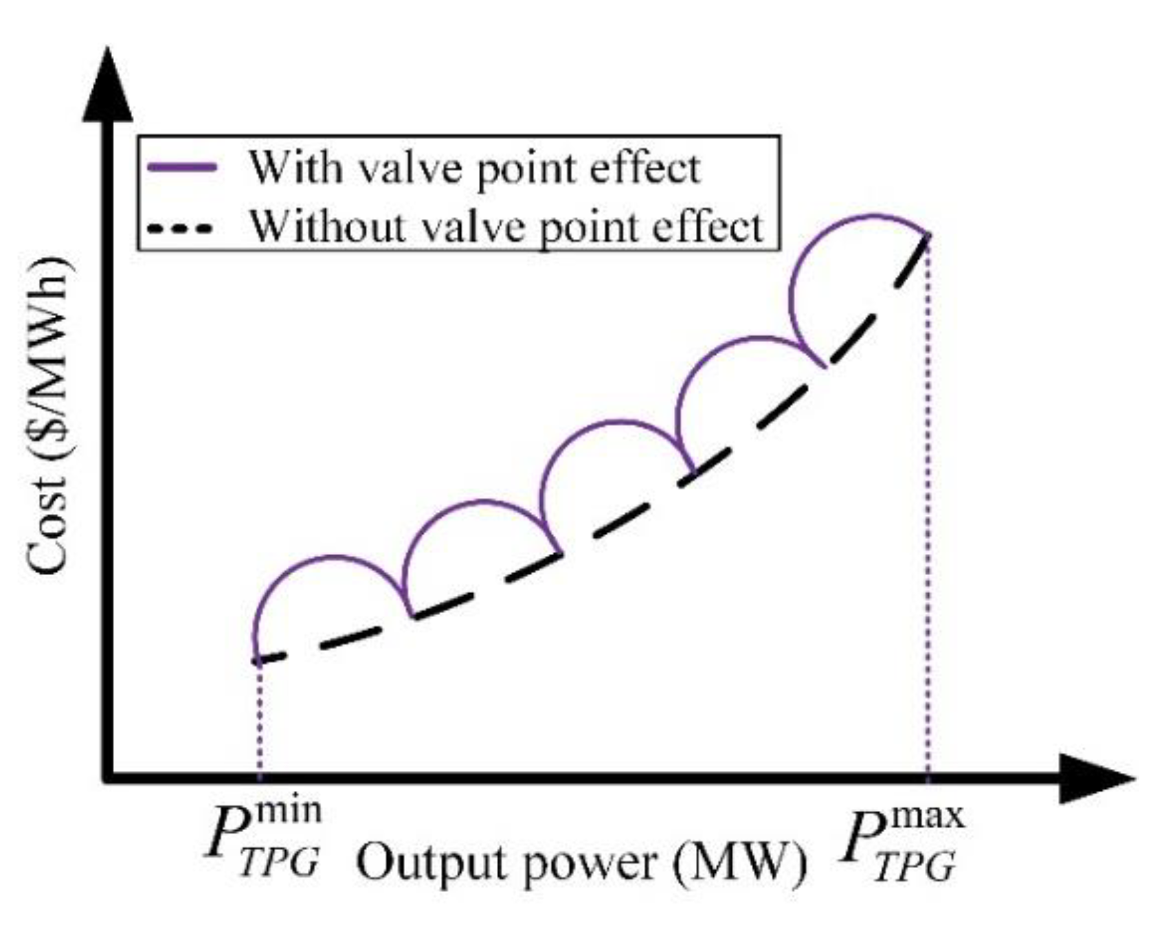
3.1.1. Fuel-Cost Study of TPG Units
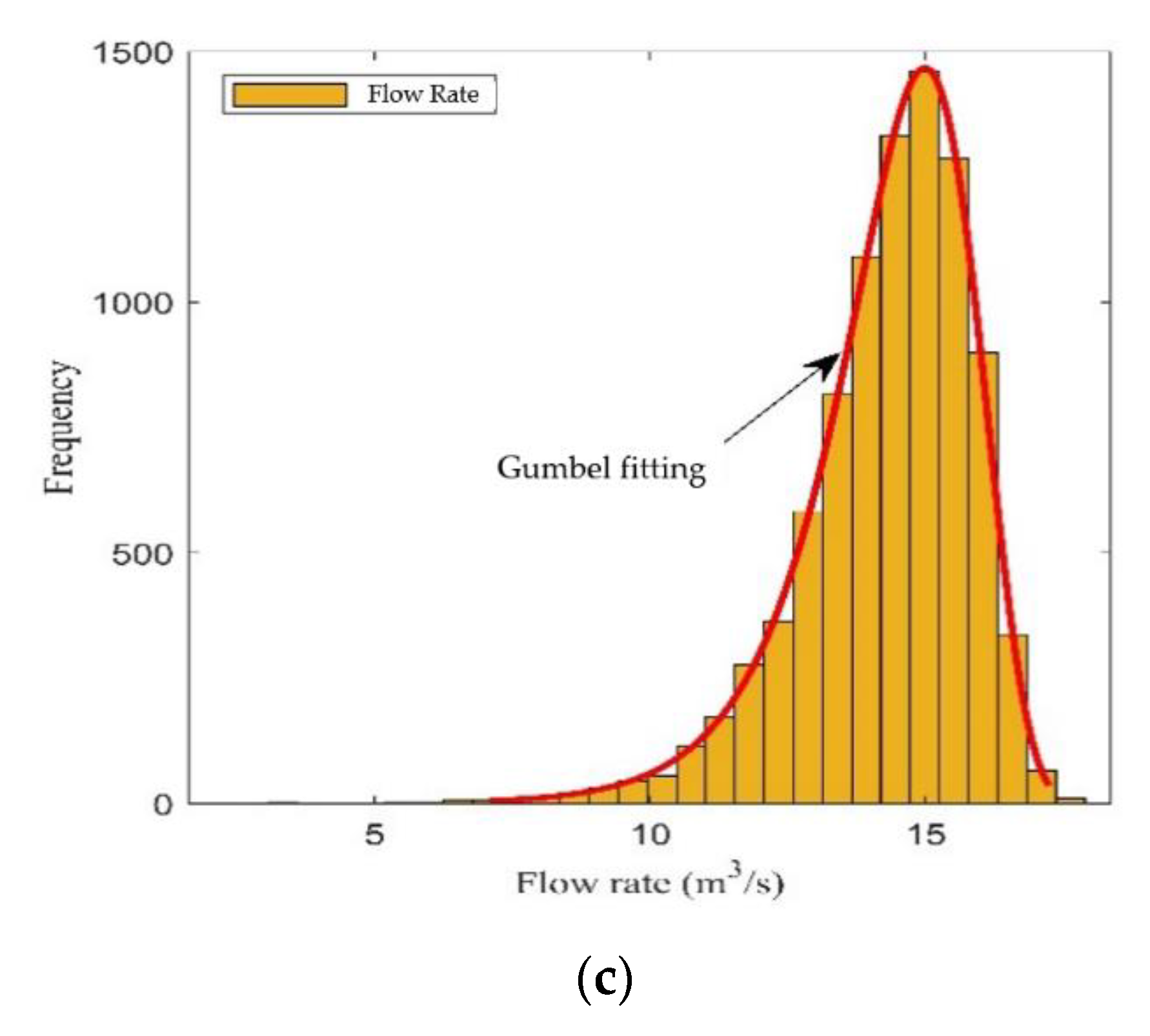
3.1.2. Fuel-Cost Study of the RESs
3.2. Emission Levels
3.3. Voltage Deviation
3.4. Power Losses
3.5. Voltage Stability Metric
3.6. Constraints
3.6.1. Power Balance
3.6.2. Limits of the Active and Reactive Powers
3.6.3. Limits of POZs
3.6.4. Security Restrictions
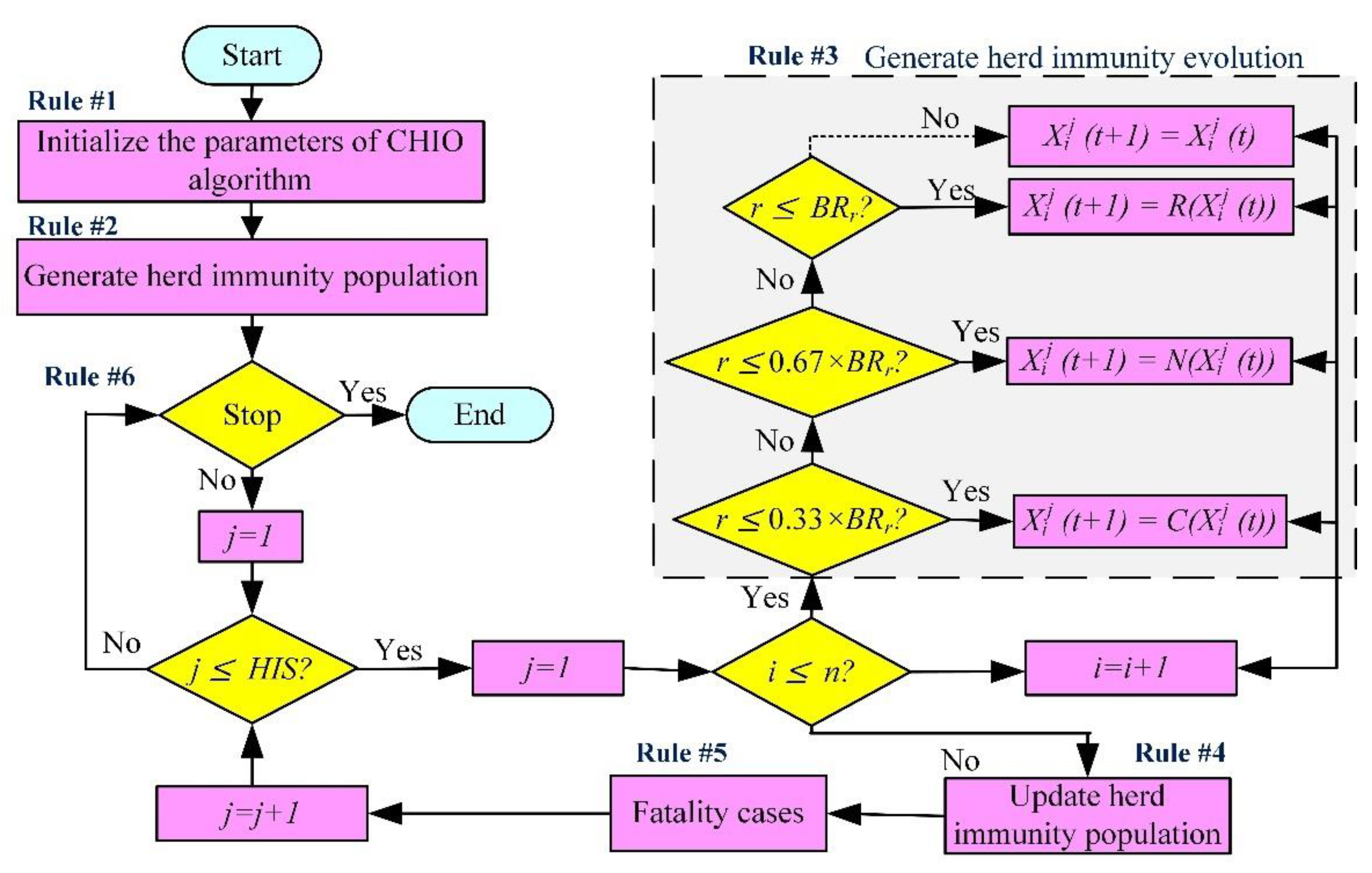
4. Coronavirus Herd Immunity Optimizer (CHIO)
4.1. Implementation Procedure of Multi-Objective CHIO
- Set the CHIO parameters; Max_Itr = 300; MaxAge = 100; popsize (HIS) = 50; C0 = 1; BRr = 0.05; lb and ub are given in each table in results.
- Assess the immunological position of herd X using the Pareto sorting algorithm.
- Obtain the non-dominated solution of the objective function as given in Equations (23), (25)–(28) together or individually, according to the implemented scenario.
- Collect them in the Pareto archive and determine the crowding space for every archive member.
- The Pareto sorting system is utilized for assessing the best person (non-dominated solution alone) in the archive, removing dominated alternatives from the archive.
- The population located in the CHIO method is modernized with Equation (49).
- Modernize the iteration cycle t to t = t + 1.
- Return to Rule #2 if t is less than Max_Itr. The actual positions will be assessed and the ideal Pareto front will be returned.
- Find the best solutions for the Pareto sorting system.
- Using a TOPSIS to obtain the one alternative that might be preferred through with the decision maker to speed up and integrate several possibilities as illustrated in the next Section 4.3.
- In addition, we can use the AHP to obtain the weighting factors with the CHIO technique to transform MO into SO function 4.2.
4.2. Analytical Hierarchy Process
4.3. A Technique for Order Preference by Similarity to Ideal Solution
4.4. Implementation Procedure of EETD Problem
- Set the input data of TPGs and RESs; WP, PV, and PVTP as given in Table 3 in addition to the parameters of RESs.
- Load the test systems of IEEE 30-bus and IEEE 57-bus from MATPOWER in Matlab.
- Formulate the objective functions for SOEETD and MOEETD problems.
- The AHP is employed with the MOEETD problem to obtain the weighting factors.
- Set the algorithm’s parameters—maximum number of iterations, search agents, …etc.
- Set the system constraints, as illustrated in Section 3.6.
- Obtain the non-dominated solutions of the OFs.
- Use a TOPSIS to obtain the best solution from the Pareto sorting system.
5. Results and Discussion
5.1. Results of IEEE 30-Bus Scheme
5.1.1. Single Objective Scenarios
5.1.2. Dual-Objective Scenarios
5.1.3. Triple-Objective Scenarios
5.1.4. Quad-Objective Scenario
5.1.5. Quanta-Objective Scenario
5.2. Results for IEEE 57-Bus Scheme
5.2.1. Single Objective Scenarios
5.2.2. Dual-Objective Scenarios “Economical and Technical Benefits”
5.2.3. Dual-Objective Scenarios “Economical and Environmental Benefits”
5.3. Evaluation of Economical-Environmental-Technical Benefits
6. Conclusions
Author Contributions
Funding
Data Availability Statement
Conflicts of Interest
Abbreviations
| ABC | Artificial bee colony |
| ABC-DP | Dynamic population-based artificial bee colony |
| AHP | Analytical hierarchy process |
| ALO | Ant lion optimizer |
| APSO | Accelerating particle swarm optimization |
| CCO | Criss-cross optimizer |
| CHIO | Coronavirus herd immunity optimizer |
| CI | Consistency index |
| CR | Consistency ratio |
| DP | Dynamic programming |
| EETD | Economical-environmental-technical dispatch |
| ES | Energy storage |
| ESCO | Enhanced sine cosine optimizer |
| GF | Gumbel fitting |
| HIP | Herd immunity population |
| HIS | Herd immunity size |
| ISA | Interior search algorithm |
| LF | Lognormal fitting |
| MADM | Multi-attribute decision making |
| MIL | Mixed-integer linear |
| MIQ | Mixed-integer quadratic |
| MO | Multi-objective |
| MOCE/D | Multi-objective cross-entropy algorithm based on decomposition |
| MOEA/D | Decomposition-based multi-objective evolutionary algorithm |
| MOHHO | Multi-objective Harris hawks optimization |
| MOPEO | Multi-objective population extremal optimization |
| MWOA | Modified whale optimization algorithm |
| NSGA | Non-dominated sorting genetic algorithm |
| NSGA-RL | Non-dominated sorting genetic algorithm reinforcement learning |
| ORC | Overestimation of the reservation cost |
| PDFs | Probability density functions |
| POZs | Prohibited operating zones |
| PSO | Particle swarm optimization |
| PV | photovoltaic |
| PVTP | Photovoltaic and tidal power |
| RC | Relative closeness |
| RESs | Renewable energy sources |
| RI | Average random index |
| SMODE | Summation based multi-objective differential evolution |
| SO | Single objective |
| SOS | Symbiotic organisms search |
| SPG | Standby power generation |
| SSA | Salp swarm algorithm |
| TLBO | Teaching learning-based optimization |
| TOPSIS | The technique for order preference by similarity to an ideal solution |
| TP | Tidal power |
| TPGs | Thermal power generations |
| TVAC | Time-varying acceleration coefficient |
| UPC | Underestimation of the penalty cost |
| VD | Voltage deviation |
| WF | Weibull fitting |
| WP | Wind power |
Nomenclature
| The scale factor of the wind turbine | |
| The shape factor of the wind turbine | |
| The direct cost of the photovoltaic system | |
| The direct cost of the photovoltaic-tidal power system | |
| The direct cost of the wind turbine | |
| The reserve capacity cost of the photovoltaic system | |
| The reserve capacity cost of the photovoltaic-small hydro system | |
| The reserve capacity cost of the wind turbine | |
| The storage units cost of the photovoltaic system | |
| The storage units cost of the photovoltaic-tidal power system | |
| The storage units cost of the wind turbine | |
| The total cost of the fuel or generation | |
| The total cost of the photovoltaic generation unit | |
| The total cost of the photovoltaic-tidal power unit | |
| The total cost of the wind turbine generation unit | |
| The total cost of the thermal power generations | |
| The total cost of the renewable energy sources | |
| The phase difference between the buses i and j | |
| Tidal efficiency turbines’ | |
| The total emission | |
| The probability of wind speed | |
| Friction factor | |
| γ | Scale parameter of the river |
| G | Solar irradiance |
| Standard solar irradiance | |
| The transconductance of branch q connected to bus i and bus j | |
| The effective pressure head for the water | |
| The direct cost parameter of the wind turbine | |
| The reserve capacity cost parameter of the wind turbine | |
| The storage unit cost parameter of the wind turbine | |
| λ | Location parameter of the river |
| -index | Stability index |
| Max_Itr | Maximum iteration number |
| Number of generator buses | |
| Number of load buses | |
| Number of branches in the network | |
| Power loss | |
| The actual power of the photovoltaic system | |
| The rated power of the photovoltaic system | |
| The scheduled power of the photovoltaic system | |
| The actual power of the photovoltaic small hydro system | |
| The scheduled power of the photovoltaic-small hydro system | |
| The minimum power of the ith thermal power generator unit | |
| The yield power from the tidal power plant | |
| The actual power of the wind turbine | |
| The rated power of the wind turbine | |
| The scheduled power of the wind turbine | |
| River flow rate | |
| Operation irradiance | |
| Water density | |
| The branches’ capacity limit | |
| The standard temperature in kelvin | |
| The wind speed | |
| The voltage of the ith on generator bus | |
| Cut-in speed of the wind turbine | |
| The voltage of the pth on load bus | |
| Cut-out speed of the wind turbine | |
| The rated speed of the wind turbine |
Appendix A
| WP | PV | PVTP | |
|---|---|---|---|
| Direct cost coefficients ($/MW) | = 1.70 | = 1.60 | = 1.50 |
| Reserve cost coefficients ($/MW) | = 3.00 | = 3.00 | = 3.00 |
| Penalty cost coefficients ($/MW) | = 1.40 | = 1.40 | = 1.40 |
| Optimization Techniques | ALO | SSA | Proposed (CHIO) |
|---|---|---|---|
| Max. iteration | 300 | 300 | 300 |
| No. of population | 50 | 50 | 50 |
| Control parameters | rand = [0, 1] | Kmin = 0.43 | C0 = 1 |
| Kmax = 0.85 | BRr = 0.05 | ||
| Independent runs | 30 | 30 | 30 |
| Decision Variables | Bounds | ||
|---|---|---|---|
| Min | Max | ||
| Active power (MW) | PTPG2 | 20 | 80 |
| PTPG5 | 10 | 60 | |
| PTPG8 | 10 | 35 | |
| PTPG11 | 10 | 60 | |
| PTPG13 | 10 | 60 | |
| Bus voltage (pu) | V1 | 0.96 | 1.10 |
| V2 | 0.96 | 1.10 | |
| V5 | 0.96 | 1.10 | |
| V8 | 0.96 | 1.10 | |
| V11 | 0.96 | 1.10 | |
| V13 | 0.96 | 1.10 | |
| Decision Variables | Bounds | ||
|---|---|---|---|
| Min | Max | ||
| Active power (MW) | PTPG1 | 80 | 200 |
| PTPG2 | 30 | 100 | |
| PTPG3 | 40 | 140 | |
| PTPG6 | 30 | 100 | |
| PTPG8 | 100 | 550 | |
| PTPG9 | 30 | 100 | |
| PTPG12 | 100 | 410 | |
| Bus voltage (pu) | V1 | 0.95 | 1.10 |
| V2 | 0.95 | 1.10 | |
| V3 | 0.95 | 1.10 | |
| V6 | 0.95 | 1.10 | |
| V8 | 0.95 | 1.10 | |
| V11 | 0.95 | 1.10 | |
| V12 | 0.95 | 1.10 | |
References
- Omar, A.I.; Khattab, N.M.; Abdel Aleem, S.H.E. Optimal strategy for transition into net-zero energy in educational buildings: A case study in El-Shorouk City, Egypt. Sustain. Energy Technol. Assess. 2022, 49, 101701. [Google Scholar] [CrossRef]
- Ahmed, E.M.; Rathinam, R.; Dayalan, S.; Fernandez, G.S.; Ali, Z.M.; Abdel Aleem, S.H.E.; Omar, A.I. A Comprehensive Analysis of Demand Response Pricing Strategies in a Smart Grid Environment Using Particle Swarm Optimization and the Strawberry Optimization Algorithm. Mathematics 2021, 9, 2338. [Google Scholar] [CrossRef]
- Elmetwaly, A.H.; ElDesouky, A.A.; Omar, A.I.; Attya Saad, M. Operation control, energy management, and power quality enhancement for a cluster of isolated microgrids. Ain Shams Eng. J. 2022, 13, 101737. [Google Scholar] [CrossRef]
- McLarty, D.; Panossian, N.; Jabbari, F.; Traverso, A. Dynamic economic dispatch using complementary quadratic programming. Energy 2019, 166, 755–764. [Google Scholar] [CrossRef]
- Zhan, J.P.; Wu, Q.H.; Guo, C.X.; Zhou, X.X. Fast λ-Iteration Method for Economic Dispatch With Prohibited Operating Zones. IEEE Trans. Power Syst. 2014, 29, 990–991. [Google Scholar] [CrossRef]
- Elsheakh, Y.; Zou, S.; Ma, Z.; Zhang, B. Decentralised gradient projection method for economic dispatch problem with valve point effect. IET Gener. Transm. Distrib. 2018, 12, 3844–3851. [Google Scholar] [CrossRef]
- Mahdi, F.P.; Vasant, P.; Kallimani, V.; Watada, J.; Fai, P.Y.S.; Abdullah-Al-Wadud, M. A holistic review on optimization strategies for combined economic emission dispatch problem. Renew. Sustain. Energy Rev. 2018, 81, 3006–3020. [Google Scholar] [CrossRef]
- Pan, S.; Jian, J.; Yang, L. A hybrid MILP and IPM approach for dynamic economic dispatch with valve-point effects. Int. J. Electr. Power Energy Syst. 2018, 97, 290–298. [Google Scholar] [CrossRef] [Green Version]
- Chen, F.; Huang, G.H.; Fan, Y.R.; Liao, R.F. A nonlinear fractional programming approach for environmental–economic power dispatch. Int. J. Electr. Power Energy Syst. 2016, 78, 463–469. [Google Scholar] [CrossRef]
- Wang, M.Q.; Gooi, H.B.; Chen, S.X.; Lu, S. A Mixed Integer Quadratic Programming for Dynamic Economic Dispatch With Valve Point Effect. IEEE Trans. Power Syst. 2014, 29, 2097–2106. [Google Scholar] [CrossRef]
- Pan, S.; Jian, J.; Chen, H.; Yang, L. A full mixed-integer linear programming formulation for economic dispatch with valve-point effects, transmission loss and prohibited operating zones. Electr. Power Syst. Res. 2020, 180, 106061. [Google Scholar] [CrossRef]
- Naderi, E.; Pourakbari-Kasmaei, M.; Cerna, F.V.; Lehtonen, M. A novel hybrid self-adaptive heuristic algorithm to handle single- and multi-objective optimal power flow problems. Int. J. Electr. Power Energy Syst. 2021, 125, 106492. [Google Scholar] [CrossRef]
- Omar, A.I.; Ali, Z.M.; Al-Gabalawy, M.; Abdel Aleem, S.H.E.; Al-Dhaifallah, M. Multi-objective environmental economic dispatch of an electricity system considering integrated natural gas units and variable renewable energy sources. Mathematics 2020, 8, 1100. [Google Scholar] [CrossRef]
- Nourianfar, H.; Abdi, H. Solving the multi-objective economic emission dispatch problems using Fast Non-Dominated Sorting TVAC-PSO combined with EMA. Appl. Soft Comput. 2019, 85, 105770. [Google Scholar] [CrossRef]
- Elsakaan, A.A.; El-Sehiemy, R.A.; Kaddah, S.S.; Elsaid, M.I. An enhanced moth-flame optimizer for solving non-smooth economic dispatch problems with emissions. Energy 2018, 157, 1063–1078. [Google Scholar] [CrossRef]
- ben oualid Medani, K.; Sayah, S.; Bekrar, A. Whale optimization algorithm based optimal reactive power dispatch: A case study of the Algerian power system. Electr. Power Syst. Res. 2018, 163, 696–705. [Google Scholar] [CrossRef]
- Karthik, N.; Parvathy, A.K.; Arul, R. Multi-objective economic emission dispatch using interior search algorithm. Int. Trans. Electr. Energy Syst. 2019, 29, e2683. [Google Scholar] [CrossRef] [Green Version]
- Chinnadurrai, C.; Victoire, T.A.A. Dynamic Economic Emission Dispatch Considering Wind Uncertainty Using Non-Dominated Sorting Crisscross Optimization. IEEE Access 2020, 8, 94678–94696. [Google Scholar] [CrossRef]
- El Sehiemy, R.A.; Selim, F.; Bentouati, B.; Abido, M.A. A novel multi-objective hybrid particle swarm and salp optimization algorithm for technical-economical-environmental operation in power systems. Energy 2020, 193, 116817. [Google Scholar] [CrossRef]
- Biswas, P.P.; Suganthan, P.N.; Qu, B.Y.; Amaratunga, G.A.J. Multiobjective economic-environmental power dispatch with stochastic wind-solar-small hydro power. Energy 2018, 150, 1039–1057. [Google Scholar] [CrossRef]
- El-Fergany, A.A.; Hasanien, H.M. Salp swarm optimizer to solve optimal power flow comprising voltage stability analysis. Neural Comput. Appl. 2020, 32, 5267–5283. [Google Scholar] [CrossRef]
- Alkoffash, M.S.; Awadallah, M.A.; Alweshah, M.; Zitar, R.A.; Assaleh, K.; Al-Betar, M.A. A Non-convex Economic Load Dispatch Using Hybrid Salp Swarm Algorithm. Arab. J. Sci. Eng. 2021, 46, 8721–8740. [Google Scholar] [CrossRef]
- Ding, M.; Chen, H.; Lin, N.; Jing, S.; Liu, F.; Liang, X.; Liu, W. Dynamic population artificial bee colony algorithm for multi-objective optimal power flow. Saudi J. Biol. Sci. 2017, 24, 703–710. [Google Scholar] [CrossRef] [PubMed]
- Liang, R.-H.; Wu, C.-Y.; Chen, Y.-T.; Tseng, W.-T. Multi-objective dynamic optimal power flow using improved artificial bee colony algorithm based on Pareto optimization. Int. Trans. Electr. Energy Syst. 2016, 26, 692–712. [Google Scholar] [CrossRef]
- Chen, M.-R.; Zeng, G.-Q.; Lu, K.-D. Constrained multi-objective population extremal optimization based economic-emission dispatch incorporating renewable energy resources. Renew. Energy 2019, 143, 277–294. [Google Scholar] [CrossRef]
- Wang, G.; Zha, Y.; Wu, T.; Qiu, J.; Peng, J.; Xu, G. Cross entropy optimization based on decomposition for multi-objective economic emission dispatch considering renewable energy generation uncertainties. Energy 2020, 193, 116790. [Google Scholar] [CrossRef]
- Duman, S.; Li, J.; Wu, L. AC optimal power flow with thermal–wind–solar–tidal systems using the symbiotic organisms search algorithm. IET Renew. Power Gener. 2021, 15, 278–296. [Google Scholar] [CrossRef]
- Bora, T.C.; Mariani, V.C.; Coelho, L.d.S. Multi-objective optimization of the environmental-economic dispatch with reinforcement learning based on non-dominated sorting genetic algorithm. Appl. Therm. Eng. 2019, 146, 688–700. [Google Scholar] [CrossRef]
- Yin, Y.; Liu, T.; He, C. Day-ahead stochastic coordinated scheduling for thermal-hydro-wind-photovoltaic systems. Energy 2019, 187, 115944. [Google Scholar] [CrossRef]
- Elattar, E.E. Environmental economic dispatch with heat optimization in the presence of renewable energy based on modified shuffle frog leaping algorithm. Energy 2019, 171, 256–269. [Google Scholar] [CrossRef]
- Attia, A.-F.; El Sehiemy, R.A.; Hasanien, H.M. Optimal power flow solution in power systems using a novel Sine-Cosine algorithm. Int. J. Electr. Power Energy Syst. 2018, 99, 331–343. [Google Scholar] [CrossRef]
- Li, X.; Wang, W.; Wang, H.; Wu, J.; Fan, X.; Xu, Q. Dynamic environmental economic dispatch of hybrid renewable energy systems based on tradable green certificates. Energy 2020, 193, 116699. [Google Scholar] [CrossRef]
- Chen, G.; Yi, X.; Zhang, Z.; Lei, H. Solving the Multi-Objective Optimal Power Flow Problem Using the Multi-Objective Firefly Algorithm with a Constraints-Prior Pareto-Domination Approach. Energies 2018, 11, 3438. [Google Scholar] [CrossRef] [Green Version]
- Ghasemi, M.; Ghavidel, S.; Ghanbarian, M.M.; Gharibzadeh, M.; Azizi Vahed, A. Multi-objective optimal power flow considering the cost, emission, voltage deviation and power losses using multi-objective modified imperialist competitive algorithm. Energy 2014, 78, 276–289. [Google Scholar] [CrossRef]
- Zhang, J.; Wang, S.; Tang, Q.; Zhou, Y.; Zeng, T. An improved NSGA-III integrating adaptive elimination strategy to solution of many-objective optimal power flow problems. Energy 2019, 172, 945–957. [Google Scholar] [CrossRef]
- Biswas, P.P.; Suganthan, P.N.; Mallipeddi, R.; Amaratunga, G.A.J. Optimal power flow solutions using differential evolution algorithm integrated with effective constraint handling techniques. Eng. Appl. Artif. Intell. 2018, 68, 81–100. [Google Scholar] [CrossRef]
- Khunkitti, S.; Siritaratiwat, A.; Premrudeepreechacharn, S.; Chatthaworn, R.; Watson, N. A Hybrid DA-PSO Optimization Algorithm for Multiobjective Optimal Power Flow Problems. Energies 2018, 11, 2270. [Google Scholar] [CrossRef] [Green Version]
- Kumari, M.S.; Maheswarapu, S. Enhanced Genetic Algorithm based computation technique for multi-objective Optimal Power Flow solution. Int. J. Electr. Power Energy Syst. 2010, 32, 736–742. [Google Scholar] [CrossRef]
- Mandal, B.; Kumar Roy, P. Multi-objective optimal power flow using quasi-oppositional teaching learning based optimization. Appl. Soft Comput. 2014, 21, 590–606. [Google Scholar] [CrossRef]
- Roy, P.K.; Paul, C. Optimal power flow using krill herd algorithm. Int. Trans. Electr. Energy Syst. 2015, 25, 1397–1419. [Google Scholar] [CrossRef]
- Hariharan, T.; Mohana Sundaram, K. Multiobjective optimal power flow using Particle Swarm Optimization. Int. J. Control Theory Appl. 2016, 9, 671–679. [Google Scholar]
- Mohamed, A.-A.A.; Mohamed, Y.S.; El-Gaafary, A.A.M.; Hemeida, A.M. Optimal power flow using moth swarm algorithm. Electr. Power Syst. Res. 2017, 142, 190–206. [Google Scholar] [CrossRef]
- Mondal, S.; Bhattacharya, A.; nee Dey, S.H. Multi-objective economic emission load dispatch solution using gravitational search algorithm and considering wind power penetration. Int. J. Electr. Power Energy Syst. 2013, 44, 282–292. [Google Scholar] [CrossRef]
- Younes, M.; Khodja, F.; Kherfane, R.L. Multi-objective economic emission dispatch solution using hybrid FFA (firefly algorithm) and considering wind power penetration. Energy 2014, 67, 595–606. [Google Scholar] [CrossRef]
- Qu, B.Y.; Liang, J.J.; Zhu, Y.S.; Wang, Z.Y.; Suganthan, P.N. Economic emission dispatch problems with stochastic wind power using summation based multi-objective evolutionary algorithm. Inf. Sci. 2016, 351, 48–66. [Google Scholar] [CrossRef]
- Zhu, Y.; Wang, J.; Qu, B. Multi-objective economic emission dispatch considering wind power using evolutionary algorithm based on decomposition. Int. J. Electr. Power Energy Syst. 2014, 63, 434–445. [Google Scholar] [CrossRef]
- Li, M.S.; Wu, Q.H.; Ji, T.Y.; Rao, H. Stochastic multi-objective optimization for economic-emission dispatch with uncertain wind power and distributed loads. Electr. Power Syst. Res. 2014, 116, 367–373. [Google Scholar] [CrossRef]
- Bilil, H.; Aniba, G.; Maaroufi, M. Probabilistic Economic Emission Dispatch Optimization of Multi-sources Power System. Energy Procedia 2014, 50, 789–796. [Google Scholar] [CrossRef] [Green Version]
- Khan, N.; Sidhu, G.; Gao, F. Optimizing Combined Emission Economic Dispatch for Solar Integrated Power Systems. IEEE Access 2016, 4, 1. [Google Scholar] [CrossRef]
- Shilaja, C.; Ravi, K. Optimization of emission/economic dispatch using euclidean affine flower pollination algorithm (eFPA) and binary FPA (BFPA) in solar photo voltaic generation. Renew. Energy 2017, 107, 550–566. [Google Scholar] [CrossRef]
- Roy, R.; Jadhav, H.T. Optimal power flow solution of power system incorporating stochastic wind power using Gbest guided artificial bee colony algorithm. Int. J. Electr. Power Energy Syst. 2015, 64, 562–578. [Google Scholar] [CrossRef]
- Rawa, M.; Abusorrah, A.; Bassi, H.; Mekhilef, S.; Ali, Z.M.; Abdel Aleem, S.H.E.; Hasanien, H.M.; Omar, A.I. Economical-technical-environmental operation of power networks with wind-solar-hydropower generation using analytic hierarchy process and improved grey wolf algorithm. Ain Shams Eng. J. 2021, 12, 2717–2734. [Google Scholar] [CrossRef]
- Mirjalili, S.; Gandomi, A.H.; Mirjalili, S.Z.; Saremi, S.; Faris, H.; Mirjalili, S.M. Salp Swarm Algorithm: A bio-inspired optimizer for engineering design problems. Adv. Eng. Softw. 2017, 114, 163–191. [Google Scholar] [CrossRef]
- Mirjalili, S. The Ant Lion Optimizer. Adv. Eng. Softw. 2015, 83, 80–98. [Google Scholar] [CrossRef]
- Biswas, P.P.; Suganthan, P.N.; Mallipeddi, R.; Amaratunga, G.A.J. Multi-objective optimal power flow solutions using a constraint handling technique of evolutionary algorithms. Soft Comput. 2020, 24, 2999–3023. [Google Scholar] [CrossRef]
- Al-Gabalawy, M.; Hosny, N.S.; Dawson, J.A.; Omar, A.I. State of charge estimation of a Li-ion battery based on extended Kalman filtering and sensor bias. Int. J. Energy Res. 2021, 45, 6708–6726. [Google Scholar] [CrossRef]
- Hulio, Z.H.; Jiang, W.; Rehman, S. Techno-Economic assessment of wind power potential of Hawke’s Bay using Weibull parameter: A review. Energy Strateg. Rev. 2019, 26, 100375. [Google Scholar] [CrossRef]
- Qais, M.H.; Hasanien, H.M.; Alghuwainem, S. Low voltage ride-through capability enhancement of grid-connected permanent magnet synchronous generator driven directly by variable speed wind turbine: A review. J. Eng. 2017, 2017, 1750–1754. [Google Scholar] [CrossRef]
- Hamilton, W.T.; Husted, M.A.; Newman, A.M.; Braun, R.J.; Wagner, M.J. Dispatch optimization of concentrating solar power with utility-scale photovoltaics. Optim. Eng. 2020, 21, 335–369. [Google Scholar] [CrossRef]
- de la Calle, A.; Bayon, A.; Pye, J. Techno-economic assessment of a high-efficiency, low-cost solar-thermal power system with sodium receiver, phase-change material storage, and supercritical CO2 recompression Brayton cycle. Sol. Energy 2020, 199, 885–900. [Google Scholar] [CrossRef]
- Gómez, Y.M.; Bolfarine, H.; Gómez, H.W. Gumbel distribution with heavy tails and applications to environmental data. Math. Comput. Simul. 2019, 157, 115–129. [Google Scholar] [CrossRef]
- Eshra, N.M.; Zobaa, A.F.; Abdel Aleem, S.H.E. Assessment of mini and micro hydropower potential in Egypt: Multi-criteria analysis. Energy Rep. 2021, 7, 81–94. [Google Scholar] [CrossRef]
- Al-Betar, M.A.; Alyasseri, Z.A.A.; Awadallah, M.A.; Abu Doush, I. Coronavirus herd immunity optimizer (CHIO). Neural Comput. Appl. 2021, 33, 5011–5042. [Google Scholar] [CrossRef] [PubMed]
- Kumar, C.; Magdalin Mary, D.; Gunasekar, T. MOCHIO: A Novel Multi-Objective Coronavirus Herd Immunity Optimization Algorithm for Solving Brushless Direct Current Wheel Motor Design Optimization Problem. Automatika 2021, 63, 149–170. [Google Scholar] [CrossRef]
- Abdel Aleem, S.H.E.; Zobaa, A.F.; Abdel Mageed, H.M. Assessment of energy credits for the enhancement of the Egyptian Green Pyramid Rating System. Energy Policy 2015, 87, 407–416. [Google Scholar] [CrossRef] [Green Version]
- Ho, W.; Ma, X. The state-of-the-art integrations and applications of the analytic hierarchy process. Eur. J. Oper. Res. 2018, 267, 399–414. [Google Scholar] [CrossRef]
- Saaty, R.W. The analytic hierarchy process—what it is and how it is used. Math. Model. 1987, 9, 161–176. [Google Scholar] [CrossRef] [Green Version]
- Beynon, M.J. Analytic Hierarchy Process. In The SAGE Dictionary of Quantitative Management Research; SAGE Publications Ltd.: London, UK, 2014; pp. 9–12. [Google Scholar]
- Deb, M.; Debbarma, B.; Majumder, A.; Banerjee, R. Performance –emission optimization of a diesel-hydrogen dual fuel operation: A NSGA II coupled TOPSIS MADM approach. Energy 2016, 117, 281–290. [Google Scholar] [CrossRef]
- Herbadji, O.; Slimani, L.; Bouktir, T. Optimal power flow with four conflicting objective functions using multiobjective ant lion algorithm: A case study of the algerian electrical network. Iran. J. Electr. Electron. Eng. 2019, 15, 94–113. [Google Scholar] [CrossRef]
- Herbadji, O.; Slimani, L.; Bouktir, T. Multi-objective optimal power flow considering the fuel cost, emission, voltage deviation and power losses using Multi-Objective Dragonfly algorithm. In Proceedings of the International Conference on Recent Advances in Electrical Systems, Bangalore, India, 16–17 March 2017; pp. 191–197. [Google Scholar]
- Zobaa, A.F.; Aleem, S.H.E.A.; Abdelaziz, A.Y. Classical and Recent Aspects of Power System Optimization; Academic Press: Cambridge, MA, USA; Elsevier: Amsterdam, The Netherlands, 2018; ISBN 9780128124413. [Google Scholar]
- Bouchekara, H.R.E.H.; Chaib, A.E.; Abido, M.A.; El-Sehiemy, R.A. Optimal power flow using an Improved Colliding Bodies Optimization algorithm. Appl. Soft Comput. J. 2016, 42, 119–131. [Google Scholar] [CrossRef]
- Shilaja, C.; Ravi, K. Optimal Power Flow Using Hybrid DA-APSO Algorithm in Renewable Energy Resources. Proc. Energy Procedia 2017, 117, 1085–1092. [Google Scholar] [CrossRef]
- Roa-Sepulveda, C.A.; Pavez-Lazo, B.J. A solution to the optimal power flow using simulated annealing. In Proceedings of the 2001 IEEE Porto Power Tech Proceedings, Porto, Portugal, 10–13 September 2001; Volume 2, pp. 5–9. [Google Scholar] [CrossRef]
- Khan, I.U.; Javaid, N.; Gamage, K.A.A.; James Taylor, C.; Baig, S.; Ma, X. Heuristic Algorithm Based Optimal Power Flow Model Incorporating Stochastic Renewable Energy Sources. IEEE Access 2020, 8, 148622–148643. [Google Scholar] [CrossRef]
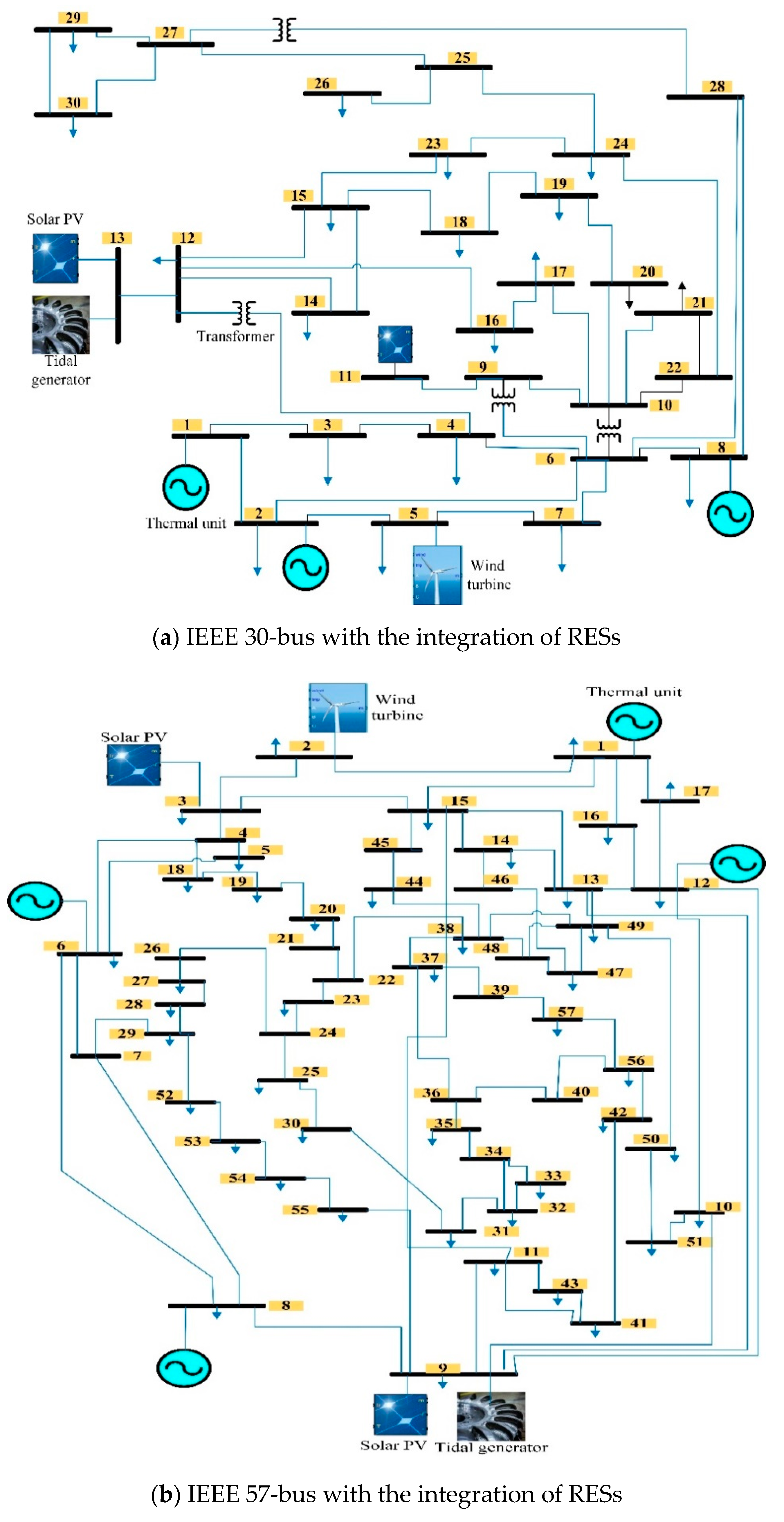


| Systems | IEEE30-Bus | IEEE57-Bus |
|---|---|---|
| Photovoltaic (PV) | Bus 11 | Bus 3 |
| Wind (WP) | Bus 5 | Bus 2 |
| PV + Tidal power (PVTP) | Bus 13 | Bus 9 |
| IEEE30-Bus | IEEE57-Bus | ||||
|---|---|---|---|---|---|
| Elements | Quantity | Parameters | Quantity | Parameters | |
| Generators | 6 | 3 TPGs and 3 RESs | 7 | 4 TPGs and 3 RESs | |
| TPGs | 3 | Buses 1(swing), 2, and 8 | 4 | Buses 1 (swing), 6, 8, and 12 | |
| RESs | PV | 25 | Bus 11, 75 MW | 75 | Bus 3, 175 MW |
| WP | 1 | Bus 5, 50 MW | 1 | Bus 2, 90 MW | |
| PVTP | 1 | Bus 13, 45 + 5 MW | 1 | Bus 9, 75 + 15 MW | |
| Static VAR compensator | 9 | Buses 10, 12, 15, 17, 20, 21, 23, 24, and 29 | 3 | Buses 18, 25, and 53 | |
| Load connected (P and Q) | - | 283.40 MW and 126.20 MVAr | - | 1250.80 MW and 336.40 MVAr | |
| Number of PQ buses | 24 | 24 buses | 50 | 50 buses | |
| Load voltage permissible range (pu) | - | 0.950–1.10 | - | 0.950–1.10 | |
| Test System | EETD Formulation | Economical | Environmental | Technical | |||
|---|---|---|---|---|---|---|---|
| No. of Objective Functions | Scenario | Fuel Costs | Emissions | VD | Ploss | L-Max | |
| IEEE-30 | 1 | 1 | ✓ | ||||
| 2 | ✓ | ||||||
| 3 | ✓ | ||||||
| 4 | ✓ | ||||||
| 5 | ✓ | ||||||
| 2 | 6 | ✓ | ✓ | ||||
| 7 | ✓ | ✓ | |||||
| 8 | ✓ | ✓ | |||||
| 3 | 9 | ✓ | ✓ | ✓ | |||
| 10 | ✓ | ✓ | ✓ | ||||
| 11 | ✓ | ✓ | ✓ | ||||
| 4 | 12 | ✓ | ✓ | ✓ | ✓ | ||
| 5 | 13 | ✓ | ✓ | ✓ | ✓ | ✓ | |
| IEEE-57 | 1 | 14 | ✓ | ||||
| 2 | 15 | ✓ | ✓ | ||||
| 16 | ✓ | ✓ | |||||
| Emission coefficients | ||||||
| Generators | Bus | (t/h) | (t/pu·MWh) | (t/pu·MW2h) | ||
| IEEE 30-bus | ||||||
| TPG1 | 1 | 0.04092 | −0.05553 | 0.0649 | 0.0003 | 6.668 |
| TPG2 | 2 | 0.02543 | −0.06048 | 0.05639 | 0.0006 | 3.334 |
| TPG3 | 8 | 0.05327 | −0.0356 | 0.0339 | 0.003 | 2 |
| IEEE 57-bus | ||||||
| TPG1 | 1 | 4.091 | −5.554 | 6.49 | 0.0002 | 0.286 |
| TPG2 | 6 | 2.543 | −6.047 | 5.638 | 0.0005 | 0.333 |
| TPG3 | 8 | 6.131 | −5.55 | 5.151 | 0.0001 | 0.667 |
| TPG4 | 12 | 3.491 | −5.754 | 6.39 | 0.0003 | 0.266 |
| Cost coefficients | ||||||
| Generators | Bus | ($/h) | ($/MWh) | ($/MW2h) | ($/h) | (MW−1) |
| IEEE 30-bus | ||||||
| TPG1 | 1 | 30 | 2 | 0.00377 | 18 | 0.038 |
| TPG2 | 2 | 25 | 1.76 | 0.0176 | 16 | 0.039 |
| TPG3 | 8 | 20 | 3.26 | 0.00833 | 12 | 0.046 |
| IEEE 57-bus | ||||||
| TPG1 | 1 | 0 | 20 | 0.0775795 | 18 | 0.037 |
| TPG2 | 6 | 0 | 40 | 0.01 | 16 | 0.038 |
| TPG3 | 8 | 0 | 20 | 0.02222 | 13.5 | 0.041 |
| TPG4 | 12 | 0 | 20 | 0.03226 | 18 | 0.037 |
| System | Scenario | Judgment Matrix (M) | Weights |
|---|---|---|---|
| IEEE 30-bus | 6 | 0.6667 0.3333 | |
| 7 | 0.6667 0.3333 | ||
| 8 | 0.6667 0.3333 | ||
| 9 | 0.5 0.25 0.25 | ||
| 10 | 0.44118 0.39706 0.16176 | ||
| 11 | 0.44118 0.39706 0.16176 | ||
| 12 | 0.34711 0.27273 0.27273 0.10744 | ||
| 13 | 0.29032 0.20968 0.20968 0.20968 0.080642 | ||
| IEEE 57-bus | 15 | 0.6667 0.3333 | |
| 16 | 0.6667 0.3333 |
| Variables and Parameters | Bounds | Scenario #1 | Scenario #2 | Scenario #3 | ||||||||
|---|---|---|---|---|---|---|---|---|---|---|---|---|
| Min | Max | CHIO | ALO | SSA | CHIO | ALO | SSA | CHIO | ALO | SSA | ||
| Active power (MW) | PTPG2 | 20 | 80 | 37.445 | 38.257 | 37.622 | 46.634 | 46.634 | 46.634 | 80 | 53.655 | 60.324 |
| PTPG5 | 10 | 60 | 38.714 | 38.588 | 37.862 | 60 | 58.316 | 59.684 | 60 | 56.919 | 57.537 | |
| PTPG8 | 10 | 35 | 10 | 10 | 10 | 35 | 35 | 35 | 35 | 28.991 | 34.084 | |
| PTPG11 | 10 | 60 | 40.571 | 38.336 | 41.687 | 56.043 | 59.536 | 59.257 | 29.748 | 57.191 | 55.194 | |
| PTPG13 | 10 | 60 | 31.952 | 32.236 | 32.339 | 48.609 | 47.19 | 47.433 | 10 | 17.146 | 10.21 | |
| Reactive power (MVAr) | Q2 | −20 | 60 | 10.108 | 21.867 | −20 | 60 | −6.6963 | −20 | −20 | −20 | −20 |
| Q5 | −30 | 35 | 35 | 26.714 | 35 | −30 | 35 | −1.7046 | 35 | 35 | 35 | |
| Q8 | −15 | 40 | 40 | 40 | 40 | 40 | −15 | −5.0345 | 40 | 40 | 40 | |
| Q11 | −25 | 30 | 18.137 | 18.382 | 21.412 | −6.3482 | 2.2441 | 7.1202 | 36.844 | 39.512 | 39.207 | |
| Q13 | −20 | 25 | 22.986 | 22.671 | 21.227 | 10.918 | 25 | 25 | 47.752 | 46.565 | 47.449 | |
| Bus voltage (pu) | V1 | 0.96 | 1.10 | 1.1 | 1.1 | 1.1 | 1.1 | 1.0905 | 1.0729 | 1.0489 | 1.0438 | 0.99822 |
| V2 | 0.96 | 1.10 | 1.09 | 1.0918 | 0.99286 | 1.1 | 1.0567 | 0.95162 | 0.95 | 1.0384 | 0.99455 | |
| V5 | 0.96 | 1.10 | 1.1 | 1.0722 | 1.0994 | 0.95 | 1.0876 | 0.96103 | 1.1 | 1.0993 | 1.093 | |
| V8 | 0.96 | 1.10 | 1.1 | 1.097 | 1.0971 | 1.0918 | 0.95844 | 0.96006 | 1.0877 | 1.0927 | 1.0904 | |
| V11 | 0.96 | 1.10 | 1.1 | 1.1 | 1.0991 | 0.96502 | 0.9741 | 0.95096 | 1.1 | 1.1 | 1.1 | |
| V13 | 0.96 | 1.10 | 1.1 | 1.0986 | 1.0872 | 1.0163 | 1.0434 | 1.0124 | 1.1 | 1.0973 | 1.098 | |
| Wgencost | Not applicable | 115.61 | 115.21 | 112.91 | 194.56 | 187.67 | 193.26 | 194.56 | 182.03 | 184.52 | ||
| PVgencost | 109.11 | 102.45 | 112.92 | 164.93 | 179.01 | 177.89 | 80.349 | 169.75 | 162.67 | |||
| PVTPgencost | 96.688 | 97.618 | 97.898 | 156.65 | 151.05 | 152.23 | 48.433 | 59.953 | 49.051 | |||
| Fuelvlvcost | 447.542 | 454.04 | 445.92 | 332.75 | 332.76 | 332.75 | 543.67 | 414.62 | 456.16 | |||
| Fuel costs ($/h) | 768.95 | 769.32 | 769.64 | 848.89 | 850.48 | 856.14 | 867.01 | 826.36 | 852.4 | |||
| VD (pu) | 1.1341 | 1.1054 | 0.90473 | 0.74422 | 0.83431 | 1.5518 | 0.36824 | 0.3779 | 0.3717 | |||
| Ploss (MW) | 5.54 | 5.6165 | 5.6392 | 4.2397 | 4.6292 | 5.9627 | 4.4902 | 3.9095 | 4.0356 | |||
| L-index | 0.11186 | 0.11316 | 0.12337 | 0.18187 | 0.19684 | 0.2305 | 0.07990 | 0.0799 | 0.0789 | |||
| Emissions (ton/h) | 0.15187 | 0.15363 | 0.15086 | 0.09055 | 0.09055 | 0.09055 | 0.10619 | 0.0987 | 0.0988 | |||
| Computation time (s) | 367.206 | 346.553 | 417.9415 | 361.393 | 413.8874 | 378.9375 | 538.9653 | 55.1077 | 465.364 | |||
| Scenarios | Optimizations | Fuel costs ($/h) | Emissions (ton/h) | VD (pu) | Ploss (MW) | L-Index |
|---|---|---|---|---|---|---|
| Scenario #1 | CHIO | 768.95 | 0.15187 | 1.1341 | 5.54 | 0.11186 |
| ALO | 769.32 | 0.15363 | 1.1054 | 5.6165 | 0.11316 | |
| SSA | 769.64 | 0.15086 | 0.90473 | 5.6392 | 0.12337 | |
| Scenario #2 | CHIO | 848.89 | 0.09055 | 0.74422 | 4.2397 | 0.18187 |
| ALO | 850.48 | 0.09055 | 0.83431 | 4.6292 | 0.19684 | |
| SSA | 856.14 | 0.09055 | 1.5518 | 5.9627 | 0.2305 | |
| Scenario #3 | CHIO | 867.01 | 0.10619 | 0.36824 | 4.4902 | 0.07990 |
| ALO | 826.36 | 0.0987 | 0.3779 | 3.9095 | 0.0799 | |
| SSA | 852.4 | 0.0988 | 0.3717 | 4.0356 | 0.0789 | |
| Scenario #4 | CHIO | 895.88 | 0.10281 | 1.3265 | 2.0661 | 0.1013 |
| ALO | 911.08 | 0.10922 | 1.3251 | 2.0724 | 0.10073 | |
| SSA | 872.76 | 0.095233 | 1.322 | 2.0848 | 0.10155 | |
| Scenario #5 | CHIO | 911.81 | 0.10833 | 0.4257 | 2.6828 | 0.071587 |
| ALO | 913.04 | 0.10822 | 0.42521 | 2.6832 | 0.071614 | |
| SSA | 911.05 | 0.10792 | 0.42566 | 2.667 | 0.071596 |
| Scenarios | Scenario #1 | Scenario #2 | Scenario #3 | Scenario #4 | Scenario #5 |
|---|---|---|---|---|---|
| IGWO [52] | 811.838 | 0.09783 | - | 2.3584 | - |
| DA-PSO [37] | 802.12 | 0.205 | - | 3.189 | - |
| MOALO [70] | 799.14 | - | - | - | - |
| MODA [71] | 802.32 | - | - | - | - |
| WOA-PS [71] | 799.56 | 0.206 | - | 2.967 | - |
| PSO-SSO [72] | 798.98 | 0.205 | 1.25 | 2.858 | 0.124 |
| ECBO [73] | 799.035 | - | - | - | - |
| ECHT [36] | 800.41 | 0.205 | - | 3.084 | 0.136 |
| DA-APSO [74] | 802.63 | - | - | 3.003 | - |
| MVO [75] | 799.24 | - | - | 2.881 | 0.115 |
| ALO | 769.32 | 0.090553 | 0.37794 | 2.0724 | 0.071614 |
| SSA | 769.64 | 0.090553 | 0.37173 | 2.0848 | 0.071596 |
| CHIO | 768.95 | 0.090550 | 0.36824 | 2.0661 | 0.071587 |
| Variables and Parameters | Bounds | Scenario #6 | Scenario #7 | Scenario #8 | ||||||||
|---|---|---|---|---|---|---|---|---|---|---|---|---|
| Min | Max | CHIO | ALO | SSA | CHIO | ALO | SSA | CHIO | ALO | SSA | ||
| Active power (MW) | PTPG2 | 20 | 80 | 36.731 | 36.279 | 38.165 | 37.265 | 36.304 | 38.277 | 37.393 | 37.786 | 37.368 |
| PTPG5 | 10 | 60 | 38.259 | 39.366 | 38.253 | 38.639 | 39.291 | 38.74 | 38.683 | 38.721 | 39.174 | |
| PTPG8 | 10 | 35 | 10 | 10.001 | 10.794 | 10 | 10 | 10 | 10 | 10 | 10 | |
| PTPG11 | 0 | 60 | 43.679 | 42.398 | 38.918 | 40.932 | 42.481 | 43.261 | 40.947 | 37.993 | 36.702 | |
| PTPG13 | 10 | 60 | 32.958 | 31.971 | 32.57 | 32.446 | 31.727 | 31.403 | 31.862 | 32.205 | 33.668 | |
| Reactive power (MVAr) | Q2 | −20 | 60 | 10.833 | 10.874 | 9.6167 | 18.225 | 11.811 | −20 | 11.203 | 11.39 | 19.449 |
| Q5 | −30 | 35 | 35 | 35 | 35 | 24.834 | 35 | 35 | 35 | 35 | 26.742 | |
| Q8 | −15 | 40 | 40 | 40 | 40 | 40 | 40 | 40 | 40 | 40 | 40 | |
| Q11 | −25 | 30 | 19.086 | 18.154 | 18.192 | 21.655 | 19.127 | 22.201 | 18.895 | 18.226 | 19.549 | |
| Q13 | −20 | 25 | 19.924 | 22.768 | 22.559 | 14.549 | 16.545 | 19.504 | 20.235 | 22.113 | 19.33 | |
| Bus voltage (pu) | V1 | 0.96 | 1.10 | 1.1 | 1.1 | 1.1 | 1.1 | 1.1 | 1.1 | 1.1 | 1.1 | 1.1 |
| V2 | 0.96 | 1.10 | 1.0899 | 1.0905 | 1.0897 | 1.0879 | 1.089 | 0.9585 | 1.0899 | 1.0901 | 1.09 | |
| V5 | 0.96 | 1.10 | 1.1 | 1.0996 | 1.0894 | 1.0655 | 1.1 | 1.0985 | 1.1 | 1.0993 | 1.0702 | |
| V8 | 0.96 | 1.10 | 1.1 | 1.0999 | 1.0769 | 1.1 | 1.0874 | 1.0692 | 1.1 | 1.0955 | 1.0763 | |
| V11 | 0.96 | 1.10 | 1.1 | 1.1 | 1.1 | 1.1 | 1.0966 | 1.1 | 1.1 | 1.1 | 1.1 | |
| V13 | 0.96 | 1.10 | 1.0913 | 1.0997 | 1.0987 | 1.0721 | 1.0798 | 1.0823 | 1.0919 | 1.0975 | 1.088 | |
| Wgencost | Not applicable | 114.16 | 117.71 | 114.14 | 115.37 | 117.47 | 115.7 | 115.51 | 115.63 | 117.09 | ||
| PVgencost | 119.65 | 115.73 | 104.92 | 110.19 | 115.64 | 118.66 | 110.68 | 101.58 | 98.182 | |||
| PVTPgencost | 99.824 | 96.776 | 98.611 | 98.248 | 96.042 | 95.024 | 96.568 | 97.476 | 102.11 | |||
| Fuelvlvcost | 436.16 | 439.69 | 452.51 | 445.08 | 440.45 | 441.12 | 446.73 | 454.86 | 452.84 | |||
| Fuel costs ($/h) | 769.79 | 769.91 | 770.19 | 768.89 | 769.6 | 770.5 | 769.49 | 769.55 | 770.22 | |||
| VD (pu) | 1.0767 | 1.1414 | 1.1208 | 0.87394 | 0.96677 | 0.88008 | 1.0753 | 1.1121 | 1.0101 | |||
| Ploss (MW) | 5.3788 | 5.4231 | 5.5705 | 5.4964 | 5.4415 | 5.5104 | 5.5244 | 5.6632 | 5.627 | |||
| L-index | 0.11387 | 0.11146 | 0.11234 | 0.12229 | 0.1179 | 0.12414 | 0.11259 | 0.11388 | 0.11691 | |||
| Emissions (ton/h) | 0.1478 | 0.15006 | 0.15161 | 0.15101 | 0.15036 | 0.14771 | 0.15158 | 0.15475 | 0.15446 | |||
| Execution time (s) | 385.0354 | 353.1225 | 384.7674 | 343.9965 | 348.5127 | 430.5964 | 309.6968 | 408.3730 | 391.4846 | |||
| Scenarios | Scenario #6 | Scenario #7 | Scenario #8 | ||||||
|---|---|---|---|---|---|---|---|---|---|
| Optimizations | CHIO | ALO | SSA | CHIO | ALO | SSA | CHIO | ALO | SSA |
| Fuel costs ($/h) | 769.79 | 769.91 | 770.19 | 768.89 | 769.6 | 770.5 | 769.49 | 769.55 | 770.22 |
| Emissions (ton/h) | 0.1478 | 0.1501 | 0.1516 | 0.1510 | 0.1504 | 0.1477 | 0.1516 | 0.1548 | 0.1545 |
| VD (pu) | 1.0767 | 1.1414 | 1.1208 | 0.8739 | 0.9668 | 0.8801 | 1.0753 | 1.1121 | 1.0101 |
| Ploss (MW) | 5.3788 | 5.4231 | 5.5705 | 5.4964 | 5.4415 | 5.5104 | 5.5244 | 5.6632 | 5.627 |
| L-index | 0.1139 | 0.1115 | 0.1123 | 0.1223 | 0.1179 | 0.1241 | 0.1139 | 0.1126 | 0.1169 |
| Variables and Parameters | Bounds | Scenario #6 | Scenario #7 | Scenario #8 | ||||||||
|---|---|---|---|---|---|---|---|---|---|---|---|---|
| Min | Max | CHIO | ALO | SSA | CHIO | ALO | SSA | CHIO | ALO | SSA | ||
| Active power (MW) | PTPG2 | 0 | 80 | 47.845 | 48.982 | 46.078 | 45.621 | 40.152 | 66.178 | 39.117 | 47.489 | 42.04 |
| PTPG5 | 10 | 60 | 49.719 | 53.164 | 51.233 | 24.064 | 55.8 | 40.281 | 42.978 | 42.409 | 45.261 | |
| PTPG8 | 10 | 35 | 33.338 | 29.341 | 30.902 | 22.187 | 31.809 | 26.5 | 30.152 | 33.634 | 34.153 | |
| PTPG11 | 0 | 60 | 54.086 | 54.074 | 54.865 | 38.309 | 42.535 | 39.127 | 45.717 | 55.79 | 44.429 | |
| PTPG13 | 10 | 60 | 41.396 | 42.335 | 44.852 | 20.455 | 18.392 | 21.337 | 36.454 | 36.587 | 41.89 | |
| Reactive power (MVAr) | Q2 | −20 | 60 | −19.618 | 12.779 | −20 | −20 | −20 | 60 | −20 | −20 | −20 |
| Q5 | −30 | 35 | 34.737 | 35 | 35 | 35 | 35 | −17.095 | 35 | 35 | 35 | |
| Q8 | −15 | 40 | 40 | 40 | 40 | 72.152 | 40 | 40 | 40 | 40 | 40 | |
| Q11 | −25 | 30 | 20.212 | 15.917 | 11.242 | 31.598 | 38.362 | 30 | 43.473 | 39.702 | 38.295 | |
| Q13 | −20 | 25 | 25 | 19.142 | 25 | 29.794 | 47.92 | 25 | 46.347 | 47.177 | 46.652 | |
| Bus voltage (pu) | V1 | 0.96 | 1.10 | 1.0659 | 1.0995 | 1.0533 | 0.96637 | 1.0343 | 0.97412 | 1.0226 | 1.0384 | 0.99867 |
| V2 | 0.96 | 1.10 | 1.052 | 1.0989 | 0.97869 | 0.97955 | 1.0103 | 1.0998 | 0.99434 | 1.019 | 0.96053 | |
| V5 | 0.96 | 1.10 | 1.0491 | 1.0989 | 1.0657 | 1.0446 | 1.0825 | 0.98497 | 1.0773 | 1.0997 | 1.0447 | |
| V8 | 0.96 | 1.10 | 1.0624 | 1.0995 | 1.0687 | 1.0366 | 1.0743 | 1.0966 | 1.0753 | 1.0985 | 1.0639 | |
| V11 | 0.96 | 1.10 | 1.0734 | 1.0988 | 1.0218 | 1.09 | 1.1 | 1.1 | 1.0962 | 1.1 | 1.1 | |
| V13 | 0.96 | 1.10 | 1.0808 | 1.0981 | 1.0548 | 1.0662 | 1.1 | 1.0963 | 1.0829 | 1.1 | 1.1 | |
| Wgencost | Not applicable | 154.01 | 167.18 | 159.74 | 75.685 | 177.55 | 120.69 | 129.76 | 127.81 | 137.73 | ||
| PVgencost | 157.51 | 157.62 | 160.32 | 102.42 | 116.29 | 105.3 | 126.84 | 164.06 | 122.63 | |||
| PVTPgencost | 128.89 | 132.48 | 141.83 | 66.546 | 62.286 | 68.505 | 111.31 | 111.82 | 130.62 | |||
| Fuelvlvcost | 375.16 | 359.52 | 356.61 | 559.47 | 448.08 | 512.21 | 424.55 | 406.85 | 412.72 | |||
| Fuel costs ($/h) | 815.57 | 816.8 | 818.5 | 804.13 | 804.21 | 806.7 | 792.46 | 810.54 | 803.7 | |||
| VD (pu) | 0.54468 | 1.3086 | 0.53194 | 0.37806 | 0.38057 | 0.39431 | 0.55733 | 0.39718 | 0.39866 | |||
| Ploss (MW) | 3.086 | 2.7679 | 3.2697 | 8.0997 | 4.7286 | 5.3882 | 5.0538 | 4.1804 | 4.3633 | |||
| L-index | 0.11179 | 0.1011 | 0.13014 | 0.088852 | 0.08199 | 0.1176 | 0.079419 | 0.08353 | 0.08072 | |||
| Emissions (ton/h) | 0.092838 | 0.09288 | 0.09303 | 0.17045 | 0.11515 | 0.11512 | 0.11124 | 0.09741 | 0.10176 | |||
| Computation time (s) | 1070.14 | 318.07 | 441.79 | 1260.03 | 403.06 | 501.39 | 1265.38 | 433.11 | 466.480 | |||
| Scenarios | Scenario #6 | Scenario #7 | Scenario #8 | |||
|---|---|---|---|---|---|---|
| Objective Functions | Fuel Costs ($/h) | Emissions (ton/h) | Fuel Costs ($/h) | VD (pu) | Fuel Costs ($/h) | L-Index |
| MOMICA [34] | 865.06 | 0.222 | 804.96 | 0.095 | - | - |
| MOFA-CPA [33] | 852.02 | 0.279 | - | - | - | - |
| MODA [37] | 838.604 | 0.254 | 807.2807 | 0.023 | - | - |
| PSO-SSO [72] | 834.804 | 0.243 | 803.99 | 0.094 | 830.35 | 0.125 |
| ECHT [36] | - | - | 803.72 | 0.095 | - | - |
| DA-APSO [74] | - | - | 802.63 | 0.116 | - | - |
| ALO | 769.91 | 0.15006 | 769.6 | 0.96677 | 769.55 | 0.11388 |
| SSA | 770.19 | 0.15161 | 770.5 | 0.88008 | 770.22 | 0.11259 |
| CHIO | 769.79 | 0.1478 | 768.89 | 0.87394 | 769.49 | 0.11691 |
| Variables and Parameters | Bounds | Scenario #9 | Scenario #10 | Scenario #11 | ||||||||
|---|---|---|---|---|---|---|---|---|---|---|---|---|
| Min | Max | CHIO | ALO | SSA | CHIO | ALO | SSA | CHIO | ALO | SSA | ||
| Active power (MW) | PTPG2 | 0 | 80 | 37.915 | 37.263 | 37.519 | 37.575 | 37.915 | 36.998 | 36.901 | 37.704 | 38.33 |
| PTPG5 | 10 | 60 | 39.431 | 39.388 | 39.224 | 39.494 | 39.405 | 39.785 | 38.405 | 37.865 | 36.99 | |
| PTPG8 | 10 | 35 | 10 | 10 | 10 | 10 | 10 | 10.017 | 10 | 10 | 10.183 | |
| PTPG11 | 0 | 60 | 37.924 | 38.554 | 42.819 | 41.433 | 41.144 | 42.807 | 43.679 | 37.467 | 39.543 | |
| PTPG13 | 10 | 60 | 33.009 | 33.044 | 32.741 | 32.477 | 33.166 | 32.29 | 31.781 | 33.385 | 32.736 | |
| Reactive power (MVAr) | Q2 | −20 | 60 | 18.253 | 19.472 | 16.951 | 17.964 | 18.299 | 18.561 | 18.407 | 16.73 | 17.025 |
| Q5 | −30 | 35 | 24.857 | 26.403 | 23.888 | 25.398 | 26.694 | 28.245 | 24.611 | 24.745 | 24.721 | |
| Q8 | −15 | 40 | 40 | 40 | 40 | 40 | 40 | 40 | 40 | 40 | 40 | |
| Q11 | −25 | 30 | 21.124 | 18.252 | 20.827 | 19.39 | 18.651 | 19.265 | 23.083 | 20.747 | 21.473 | |
| Q13 | −20 | 25 | 15.705 | 19.236 | 17.916 | 21.272 | 22.718 | 20.103 | 10.631 | 16.58 | 14.895 | |
| Bus voltage (pu) | V1 | 0.96 | 1.10 | 1.1 | 1.1 | 1.1 | 1.1 | 1.1 | 1.1 | 1.1 | 1.1 | 1.1 |
| V2 | 0.96 | 1.10 | 1.0882 | 1.0896 | 1.0883 | 1.0899 | 1.0909 | 1.091 | 1.0871 | 1.0872 | 1.0871 | |
| V5 | 0.96 | 1.10 | 1.0661 | 1.0692 | 1.0658 | 1.0695 | 1.072 | 1.0734 | 1.0638 | 1.0646 | 1.064 | |
| V8 | 0.96 | 1.10 | 1.0995 | 1.099 | 1.0908 | 1.1 | 1.0988 | 1.0919 | 1.098 | 1.0784 | 1.0962 | |
| V11 | 0.96 | 1.10 | 1.1 | 1.0946 | 1.1 | 1.1 | 1.1 | 1.1 | 1.1 | 1.0986 | 1.0991 | |
| V13 | 0.96 | 1.10 | 1.0758 | 1.086 | 1.0824 | 1.0934 | 1.0985 | 1.0912 | 1.0597 | 1.0774 | 1.0723 | |
| Wgencost | Not applicable | 117.92 | 117.78 | 117.25 | 118.12 | 117.83 | 119.07 | 114.63 | 112.92 | 110.18 | ||
| PVgencost | 101.29 | 102.96 | 117.07 | 112.26 | 112.23 | 116.7 | 119.65 | 100.3 | 105.73 | |||
| PVTPgencost | 100.07 | 100.15 | 99.192 | 98.338 | 100.51 | 97.759 | 96.223 | 101.19 | 99.137 | |||
| Fuelvlvcost | 450.24 | 448.3 | 436.4 | 440.65 | 439.73 | 436.03 | 439.35 | 455.56 | 453.9 | |||
| Fuel costs ($/h) | 769.19 | 769.53 | 769.91 | 769.38 | 770.3 | 769.56 | 769.85 | 769.97 | 768.95 | |||
| VD (pu) | 0.89865 | 0.96724 | 0.95242 | 1.0514 | 1.1035 | 1.0609 | 0.78891 | 0.88963 | 0.85853 | |||
| Ploss (MW) | 5.5598 | 5.547 | 5.3219 | 5.3811 | 5.367 | 5.3112 | 5.4224 | 5.6972 | 5.6488 | |||
| L-index | 0.12136 | 0.11871 | 0.11957 | 0.11559 | 0.11345 | 0.11468 | 0.1258 | 0.12208 | 0.1232 | |||
| Emissions (ton/h) | 0.15239 | 0.1525 | 0.14674 | 0.14855 | 0.14763 | 0.14732 | 0.14897 | 0.15521 | 0.15312 | |||
| Execution time (s) | 279.63 | 347.842 | 362.581 | 274.884 | 375.193 | 384.989 | 272.287 | 364.287 | 385.129 | |||
| Variables and Parameters | Bounds | Scenario #9 | Scenario #10 | Scenario #11 | ||||||||
|---|---|---|---|---|---|---|---|---|---|---|---|---|
| Min | Max | CHIO | ALO | SSA | CHIO | ALO | SSA | CHIO | ALO | SSA | ||
| Active power (MW) | PTPG2 | 0 | 80 | 45.405 | 48.361 | 62.321 | 46.448 | 53.022 | 45.228 | 57.368 | 48.538 | 49.279 |
| PTPG5 | 10 | 60 | 55.529 | 50.909 | 52.175 | 71.7 | 56.496 | 54.824 | 49.2 | 46.063 | 48.875 | |
| PTPG8 | 10 | 35 | 32.838 | 26.289 | 30.04 | 34.277 | 29.567 | 29.562 | 31.29 | 25.863 | 26.658 | |
| PTPG11 | 0 | 60 | 42.484 | 55.725 | 51.342 | 59.487 | 57.34 | 51.823 | 51.129 | 51.793 | 50.458 | |
| PTPG13 | 10 | 60 | 34.013 | 43.227 | 25.283 | 40.994 | 41.834 | 42.571 | 39.104 | 43.911 | 39.191 | |
| Reactive power (MVAr) | Q2 | −20 | 60 | −20 | 15.13 | −20 | 13.944 | −3.0635 | −20 | −20 | −2.0587 | 32.849 |
| Q5 | −30 | 35 | 35 | 32.075 | 35 | 23.902 | 34.535 | 35 | 35 | 35 | 19.43 | |
| Q8 | −15 | 40 | 40 | 40 | 40 | 40 | 40 | 40 | 33.567 | 40 | 40 | |
| Q11 | −25 | 30 | 23.42 | 19.691 | 21.981 | 17.235 | 16.358 | 11.408 | 25.992 | 19.223 | 18.668 | |
| Q13 | −20 | 25 | 18.363 | 12.202 | 25 | 19.746 | 18.545 | 18.641 | 24.103 | 21.071 | 25 | |
| Bus voltage (pu) | V1 | 0.96 | 1.10 | 1.0745 | 1.0734 | 1.0649 | 1.095 | 1.0915 | 1.0813 | 1.0526 | 1.0631 | 1.0155 |
| V2 | 0.96 | 1.10 | 1.0537 | 1.0697 | 1.0252 | 1.0947 | 1.0846 | 1.0137 | 0.96787 | 1.054 | 1.0201 | |
| V5 | 0.96 | 1.10 | 1.0716 | 1.0596 | 1.0815 | 1.0859 | 1.0813 | 1.0654 | 1.0569 | 1.0653 | 0.99491 | |
| V8 | 0.96 | 1.10 | 1.0651 | 1.0713 | 1.0763 | 1.0983 | 1.0869 | 1.0725 | 1.0326 | 1.0621 | 1.0204 | |
| V11 | 0.96 | 1.10 | 1.0899 | 1.0729 | 1.0787 | 1.097 | 1.0851 | 1.0479 | 1.0754 | 1.0661 | 1.025 | |
| V13 | 0.96 | 1.10 | 1.065 | 1.0468 | 1.0787 | 1.0955 | 1.0831 | 1.059 | 1.0594 | 1.0612 | 1.0585 | |
| Wgencost | Not applicable | 176.48 | 158.51 | 163.35 | 244.28 | 180.33 | 173.68 | 152.07 | 140.59 | 150.86 | ||
| PVgencost | 115.16 | 163.95 | 147.25 | 177.97 | 169.19 | 148.74 | 146.02 | 149.08 | 143.64 | |||
| PVTPgencost | 103.26 | 135.73 | 77.989 | 127.38 | 130.44 | 133.12 | 120.58 | 138.35 | 120.81 | |||
| Fuelvlvcost | 406.04 | 355.05 | 429.43 | 308.98 | 349.31 | 357.93 | 397.85 | 376.03 | 386.85 | |||
| Fuel costs ($/h) | 800.93 | 813.24 | 818.02 | 858.61 | 829.27 | 813.47 | 816.52 | 804.05 | 802.16 | |||
| VD (pu) | 0.59367 | 0.50992 | 0.53133 | 1.2231 | 0.96821 | 0.48706 | 0.43323 | 0.46179 | 0.73504 | |||
| Ploss (MW) | 3.3057 | 3.06 | 3.326 | 1.9072 | 2.5598 | 3.0963 | 3.2613 | 3.5004 | 3.7856 | |||
| L-index | 0.11386 | 0.11634 | 0.11076 | 0.10076 | 0.10914 | 0.12837 | 0.11684 | 0.11521 | 0.12004 | |||
| Emissions (ton/h) | 0.09912 | 0.09411 | 0.09662 | 0.091123 | 0.09144 | 0.09394 | 0.093589 | 0.09718 | 0.09799 | |||
| Computation time (s) | 995.1156 | 318.7531 | 524.7601 | 1000.5954 | 302.5808 | 425.4336 | 1186.5667 | 322.3311 | 431.3868 | |||
| Scenarios | Scenario #9 | Scenario #10 | Scenario #11 | ||||||
|---|---|---|---|---|---|---|---|---|---|
| Objective Functions | Fuel Costs ($/h) | VD (pu) | Power Losses (MW) | Fuel Costs ($/h) | Emissions (ton/h) | Power Losses (MW) | Fuel Costs ($/h) | Emissions (ton/h) | VD (pu) |
| MOFA-CPA [33] | - | - | - | 878.13 | 0.2165 | 3.9232 | - | - | - |
| MODA [37] | - | - | - | 867.9070 | 0.2640 | 4.5342 | - | - | - |
| PSO-SSO [72] | 864.27 | 0.316 | 4.545 | 865.18 | 0.224 | 4.093 | 804.332 | 0.346 | 0.164 |
| ALO | 769.19 | 0.96724 | 5.547 | 770.3 | 0.14763 | 5.367 | 769.97 | 0.15521 | 0.88963 |
| SSA | 769.91 | 0.95242 | 5.3219 | 769.56 | 0.14732 | 5.3112 | 768.95 | 0.15312 | 0.85853 |
| CHIO | 769.53 | 0.89865 | 5.5598 | 769.38 | 0.14855 | 5.3811 | 769.85 | 0.14897 | 0.78891 |
| Variables and Parameters | Min. | Max. | CHIO | ALO | SSA | |
|---|---|---|---|---|---|---|
| Active power (MW) | PTG2 | 20 | 80 | 48.714 | 50.953 | 47.125 |
| PTG5 | 10 | 60 | 48.81 | 54.609 | 50.637 | |
| PTG8 | 10 | 35 | 27.752 | 33.426 | 31.178 | |
| PTG11 | 10 | 60 | 54.453 | 48.113 | 54.953 | |
| PTG13 | 10 | 48.652 | 39.445 | 36.464 | 43.843 | |
| Reactive power (MVAr) | Q2 | −20 | 60 | 33.559 | 6.7174 | −20 |
| Q5 | −30 | 35 | 26.541 | 35 | 28.401 | |
| Q8 | −15 | 40 | 40 | 38.79 | 40 | |
| Q11 | −25 | 30 | 16.525 | 17.953 | 16.23 | |
| Q13 | −20 | 25 | 14.031 | 14.739 | 12.23 | |
| Bus voltage (pu) | V1 | 0.96 | 1.10 | 1.071 | 1.0769 | 1.0804 |
| V2 | 0.96 | 1.10 | 1.0723 | 1.0716 | 0.99356 | |
| V5 | 0.96 | 1.10 | 1.0543 | 1.074 | 1.0452 | |
| V8 | 0.96 | 1.10 | 1.0697 | 1.0619 | 1.05 | |
| V11 | 0.96 | 1.10 | 1.0634 | 1.0759 | 1.0526 | |
| V13 | 0.96 | 1.10 | 1.0499 | 1.0581 | 1.0363 | |
| Wgencost | Not applicable | 150.62 | 172.84 | 157.47 | ||
| PVgencost | 159.28 | 134.89 | 160.63 | |||
| PVTPgencost | 121.73 | 111.72 | 138.18 | |||
| Fuelvlvcost | 375.46 | 392.93 | 361.45 | |||
| Total cost ($/h) | 807.09 | 812.37 | 817.74 | |||
| VD (pu) | 0.4942 | 0.59979 | 0.46338 | |||
| Ploss (MW) | 3.2669 | 2.9596 | 3.1828 | |||
| L-index | 0.11517 | 0.11298 | 0.13688 | |||
| Emission (ton/h) | 0.095747 | 0.093889 | 0.092843 | |||
| Computation time (s) | 1070.1630 | 302.5195 | 404.1681 | |||
| Variables and Parameters | Min | Max | CHIO | ALO | SSA | |
|---|---|---|---|---|---|---|
| Active power (MW) | PTG2 | 20 | 80 | 73.507 | 47.479 | 47.016 |
| PTG5 | 10 | 60 | 54.844 | 45.5 | 47.761 | |
| PTG8 | 10 | 35 | 33.146 | 25.043 | 33.585 | |
| PTG11 | 10 | 60 | 56.072 | 46.144 | 46.941 | |
| PTG13 | 10 | 48.652 | 38.813 | 35.025 | 40.565 | |
| Reactive power (MVAr) | Q2 | −20 | 60 | −20 | 1.6023 | 33.452 |
| Q5 | −30 | 35 | 35 | 31.742 | 6.0559 | |
| Q8 | −15 | 40 | 40 | 40 | 40 | |
| Q11 | −25 | 30 | 37.94 | 20.115 | 24.597 | |
| Q13 | −20 | 25 | 44.923 | 25 | 25 | |
| Bus voltage (pu) | V1 | 0.96 | 1.10 | 1.0326 | 1.0659 | 1.0516 |
| V2 | 0.96 | 1.10 | 0.97156 | 1.0572 | 1.0502 | |
| V5 | 0.96 | 1.10 | 1.0951 | 1.0475 | 1.0134 | |
| V8 | 0.96 | 1.10 | 1.0909 | 1.0718 | 1.0592 | |
| V11 | 0.96 | 1.10 | 1.0948 | 1.0763 | 1.0775 | |
| V13 | 0.96 | 1.10 | 1.0941 | 1.0916 | 1.0695 | |
| Wgencost | Not applicable | 173.76 | 138.58 | 146.75 | ||
| PVgencost | 164.98 | 128.43 | 131.24 | |||
| PVTPgencost | 119.51 | 106.59 | 125.99 | |||
| Fuelvlvcost | 406 | 414.66 | 400.5 | |||
| Total cost ($/h) | 864.25 | 788.26 | 804.47 | |||
| VD (pu) | 0.39559 | 0.55259 | 0.42219 | |||
| Ploss (MW) | 3.1204 | 3.9664 | 3.4982 | |||
| L-index | 0.075979 | 0.11077 | 0.10948 | |||
| Emission (ton/h) | 0.096721 | 0.10653 | 0.096649 | |||
| Computation time (s) | 991.7640 | 347.8191 | 358.4133 | |||
| Scenarios | Scenario #12 | Scenario #13 | |||||||
|---|---|---|---|---|---|---|---|---|---|
| Objective Functions | Fuel Costs ($/h) | Emission (ton/h) | VD (pu) | Power Losses (MW) | Fuel Costs ($/h) | Emissions (ton/h) | VD (pu) | Power Losses (MW) | L-Index |
| MOMICA [34] | 830.188 | 0.252 | 0.298 | 5.585 | - | - | - | - | - |
| I-NSGA-III [35] | 881.9395 | 0.2209 | 0.1754 | 4.7449 | 843.8571 | 0.1485 | 0.2388 | 5.7405 | 0.1253 |
| MODA [37] | 828.49 | 0.265 | 0.585 | 5.912 | - | - | - | - | - |
| ECHT [36] | 830.2123 | 0.253 | 0.296 | 5.586 | - | - | - | - | - |
| PSO-SSO [72] | 826.94 | 0.258 | 0.466 | 5.515 | 826.8 | 0.256 | 0.463 | 5.464 | 0.145 |
| ALO | 769.07 | 0.14957 | 0.84792 | 5.5493 | 769.93 | 0.14867 | 0.97541 | 5.3714 | 0.11758 |
| SSA | 770.43 | 0.14799 | 0.83337 | 5.4257 | 770.18 | 0.15455 | 0.8247 | 5.6446 | 0.12473 |
| CHIO | 768.92 | 0.15177 | 0.92664 | 5.4395 | 770.13 | 0.14624 | 0.86862 | 5.3023 | 0.12242 |
| Variables and Parameters | Bounds | Scenario #14 | ||||
|---|---|---|---|---|---|---|
| Min | Max | CHIO | ALO | SSA | ||
| Active power (MW) | PTPG1 | 80 | 200 | 142.03 | 143.32 | 142.02 |
| PTPG2 | 30 | 100 | 100 | 100 | 100 | |
| PTPG3 | 40 | 140 | 140 | 140 | 140 | |
| PTPG6 | 30 | 100 | 90.462 | 99.915 | 85.404 | |
| PTPG8 | 100 | 550 | 381.24 | 375.31 | 384.08 | |
| PTPG9 | 30 | 100 | 48.64 | 48.587 | 48.605 | |
| PTPG12 | 100 | 410 | 362.39 | 362.87 | 364.11 | |
| Reactive power (MVAr) | Q2 | −17 | 50 | 46.138 | 49.685 | 50 |
| Q3 | −10 | 60 | 29.639 | 28.616 | −10 | |
| Q6 | −8 | 25 | 5.0015 | 1.2401 | −8 | |
| Q8 | −140 | 200 | 42.065 | 40.539 | 69.403 | |
| Q9 | −3 | 9 | 5 | 9 | −3 | |
| Q12 | −150 | 155 | 56.541 | 67.292 | 69.611 | |
| Bus voltage (pu) | V1 | 0.95 | 1.10 | 1.1 | 1.0991 | 1.1 |
| V2 | 0.95 | 1.10 | 1.1 | 1.1 | 1.0999 | |
| V3 | 0.95 | 1.10 | 1.1 | 1.1 | 1.0078 | |
| V6 | 0.95 | 1.10 | 1.1 | 1.0994 | 0.9591 | |
| V8 | 0.95 | 1.10 | 1.1 | 1.1 | 1.1 | |
| V11 | 0.95 | 1.10 | 1.1 | 1.098 | 1.0423 | |
| V12 | 0.95 | 1.10 | 1.0821 | 1.0865 | 1.0823 | |
| Wgencost | Not applicable | 555.43 | 555.43 | 555.43 | ||
| PVgencost | 1646.6 | 1616.9 | 1658.4 | |||
| PVTPgencost | 156.77 | 156.57 | 156.63 | |||
| Fuelvlvcost | 30,393 | 30,427 | 30,399 | |||
| Fuel costs ($/h) | 32,752 | 32,756 | 32,770 | |||
| VD (pu) | 4.9146 | 4.9821 | 4.5556 | |||
| Ploss (MW) | 12.738 | 12.708 | 13.098 | |||
| L-index | 0.2321 | 0.2294 | 0.2417 | |||
| Emissions (ton/h) | 1.2322 | 1.2582 | 1.2763 | |||
| Computation time (s) | 347.42 | 399.24 | 609.65 | |||
| Variables and Parameters | Bounds | Scenario #15—AHP | Scenario #15—TOPSIS | ||||||
|---|---|---|---|---|---|---|---|---|---|
| Min | Max | CHIO | ALO | SSA | CHIO | ALO | SSA | ||
| Active power (MW) | PTPG1 | 80 | 200 | 141.13 | 146.85 | 142.12 | |||
| PTPG2 | 30 | 100 | 100 | 100 | 100 | 97.284 | 99.802 | 99.991 | |
| PTPG3 | 40 | 140 | 140 | 140 | 140 | 136.61 | 139.98 | 140 | |
| PTPG6 | 30 | 100 | 90.525 | 66.72 | 64.232 | 66.124 | 75.725 | 49.604 | |
| PTPG8 | 100 | 550 | 381.28 | 391.52 | 390.9 | 394.54 | 400.59 | 342.82 | |
| PTPG9 | 30 | 100 | 48.555 | 48.524 | 48.595 | 47.437 | 48.526 | 48.244 | |
| PTPG12 | 100 | 410 | 362.39 | 374 | 375.88 | 349.16 | 360.12 | 406.63 | |
| Reactive power (MVAr) | Q2 | −17 | 50 | 50 | 47.376 | 50 | 50 | 50 | −17 |
| Q3 | −10 | 60 | 30.456 | 28.034 | −10 | 32.267 | −10 | 35.239 | |
| Q6 | −8 | 25 | 5.0223 | 9.0762 | −8 | −8 | 25 | 25 | |
| Q8 | −140 | 200 | 42.625 | 37.959 | 63.327 | 45.618 | 13.908 | 28.807 | |
| Q9 | −3 | 9 | 9 | 9 | 9 | 9 | 9 | 9 | |
| Q12 | −150 | 155 | 56.269 | 63.386 | 65.015 | 139.05 | 155 | 155 | |
| Bus voltage (pu) | V1 | 0.95 | 1.10 | 1.099 | 1.0996 | 1.1 | 1.0096 | 1.0153 | 0.99824 |
| V2 | 0.95 | 1.10 | 1.1 | 1.1 | 1.0977 | 1.0274 | 1.038 | 0.95031 | |
| V3 | 0.95 | 1.10 | 1.1 | 1.1 | 0.9876 | 1.0113 | 0.99729 | 1.003 | |
| V6 | 0.95 | 1.10 | 1.1 | 1.0991 | 1.0437 | 0.99375 | 1.0266 | 1.0878 | |
| V8 | 0.95 | 1.10 | 1.1 | 1.1 | 1.1 | 1.0164 | 1.0094 | 1.0091 | |
| V11 | 0.95 | 1.10 | 1.1 | 1.1 | 1.099 | 1.0247 | 1.0577 | 1.0997 | |
| V12 | 0.95 | 1.10 | 1.0815 | 1.0866 | 1.0836 | 1.0257 | 1.0426 | 1.0941 | |
| Wgencost | Not applicable | 555.43 | 555.43 | 555.43 | 539.82 | 555.32 | 555.43 | ||
| PVgencost | 1645.4 | 1691.9 | 1689.8 | 1706.3 | 1732.7 | 1468.1 | |||
| PVTPgencost | 156.45 | 156.33 | 156.6 | 152.24 | 156.33 | 155.27 | |||
| Fuelvlvcost | 30,397 | 30,367 | 30,384 | 30,900 | 30,490 | 31,052 | |||
| Fuel costs ($/h) | 32,754 | 32,771 | 32,786 | 33,299 | 32,935 | 33,230 | |||
| VD (pu) | 4.8974 | 4.9926 | 4.6149 | 1.0707 | 1.0937 | 1.0872 | |||
| Ploss (MW) | 12.736 | 12.458 | 12.717 | 16.833 | 16.794 | 16.379 | |||
| L-index | 0.23147 | 0.22979 | 0.2404 | 0.26182 | 0.26843 | 0.25241 | |||
| Emissions (ton/h) | 1.2584 | 1.341 | 1.3454 | 1.3261 | 1.3465 | 1.3064 | |||
| Computation time (s) | 427.4885 | 414.6923 | 596.62 | 1303.38 | 455.579 | 560.509 | |||
| Variables and Parameters | Bounds | Scenario #16—AHP | Scenario #16—TOPSIS | ||||||
|---|---|---|---|---|---|---|---|---|---|
| Min | Max | CHIO | ALO | SSA | CHIO | ALO | SSA | ||
| Active power (MW) | PTPG1 | 80 | 200 | 140.44 | 142.84 | 158.66 | 140.44 | 142.84 | 158.66 |
| PTPG2 | 30 | 100 | 100 | 100 | 100 | 100 | 100 | 99.849 | |
| PTPG3 | 40 | 140 | 140 | 140 | 140 | 139.99 | 140 | 139.99 | |
| PTPG6 | 30 | 100 | 90.488 | 95.416 | 65.626 | 99.938 | 100 | 99.78 | |
| PTPG8 | 100 | 550 | 381.21 | 384.31 | 392.53 | 320.04 | 336.72 | 320.58 | |
| PTPG9 | 30 | 100 | 48.653 | 48.614 | 48.601 | 48.609 | 48.671 | 48.578 | |
| PTPG12 | 100 | 410 | 362.38 | 357.39 | 372.12 | 339.96 | 345.59 | 334.15 | |
| Reactive power (MVAr) | Q2 | −17 | 50 | 46.138 | 49.066 | 49.93 | 45.377 | 45.545 | 30.186 |
| Q3 | −10 | 60 | 29.64 | 28.429 | 30.756 | 26.853 | 21.835 | −4.2581 | |
| Q6 | −8 | 25 | 4.9955 | 3.4006 | 10.004 | 7.0424 | 4.1125 | −8 | |
| Q8 | −140 | 200 | 42.068 | 39.15 | 47.067 | 44.505 | 35.441 | 83.674 | |
| Q9 | −3 | 9 | 9 | 9 | −3 | 9 | 9 | 9 | |
| Q12 | −150 | 155 | 56.541 | 67.055 | 61.353 | 80.818 | 102.34 | 48.528 | |
| Bus voltage (pu) | V1 | 0.95 | 1.10 | 1.1 | 1.0993 | 1.099 | 1.0995 | 1.1 | 1.0934 |
| V2 | 0.95 | 1.10 | 1.1 | 1.1 | 1.1 | 1.0994 | 1.1 | 1.0852 | |
| V3 | 0.95 | 1.10 | 1.1 | 1.1 | 1.1 | 1.0992 | 1.1 | 1.0724 | |
| V6 | 0.95 | 1.10 | 1.1 | 1.1 | 1.0992 | 1.0995 | 1.1 | 1.0496 | |
| V8 | 0.95 | 1.10 | 1.1 | 1.1 | 1.1 | 1.0987 | 1.1 | 1.0915 | |
| V11 | 0.95 | 1.10 | 1.1 | 1.0999 | 0.9527 | 1.0968 | 1.1 | 1.0907 | |
| V12 | 0.95 | 1.10 | 1.0821 | 1.0858 | 1.0833 | 1.0887 | 1.1 | 1.0614 | |
| Wgencost | Not applicable | 555.43 | 555.43 | 555.43 | 555.39 | 555.43 | 555.36 | ||
| PVgencost | 1645.4 | 1658.3 | 1696.8 | 1363.1 | 1439.8 | 1365.3 | |||
| PVTPgencost | 156.82 | 156.67 | 156.62 | 156.65 | 156.9 | 156.54 | |||
| Fuelvlvcost | 30,393 | 30,383 | 30,363 | 31,269 | 30,897 | 31,395 | |||
| Fuel costs ($/h) | 32,751 | 32,753 | 32,772 | 33,344 | 33,049 | 33,473 | |||
| VD (pu) | 4.9146 | 4.9718 | 4.8841 | 4.9968 | 5.2342 | 3.8727 | |||
| Ploss (MW) | 12.738 | 12.968 | 12.601 | 14.258 | 13.762 | 15.241 | |||
| L-index | 0.2321 | 0.2298 | 0.2317 | 0.22947 | 0.22395 | 0.25315 | |||
| Emissions (ton/h) | 1.2553 | 1.2581 | 1.3422 | 1.0976 | 1.1198 | 1.0964 | |||
| Computation time (s) | 422.21 | 404.68 | 488.94 | 1575.13 | 402.319 | 477.557 | |||
| System | Scenario # | IEEE without RESs | IEEE Integrated with RESs | Saving Difference with and without RESs | |||||||
|---|---|---|---|---|---|---|---|---|---|---|---|
| Competitive Techniques | Savings ($/h) | Annual Savings ($/yr.) | Competitive Techniques | Savings ($/h) | Annual Savings ($/yr.) | Savings ($/h) | Annual Savings ($/yr.) | ||||
| IEEE 30-bus | 1 | PSO-SSO [72] | 798.98 | 0.0550 | 481.80 | CHIO | 768.95 | 12.45 | 109,062 | 30.03 | 263,062.8 |
| ECBO [73] | 799.035 | GWO [76] | 781.40 | ||||||||
| 6 | PSO-SSO [72] | 834.804 | 0.110 | 963.60 | CHIO | 769.79 | 12.51 | 109,588 | 65.014 | 569,522.6 | |
| MVO [75] | 834.95 | SHADE [76] | 782.30 | ||||||||
| IEEE 57-bus | 14 | PSO-SSO [72] | 41,666.66 | 7.96 | 69,729.6 | CHIO | 32,752 | 4 | 35,040 | 8914.66 | 78,092,421.6 |
| DA-PSO [37] | 41,674.62 | ALO | 32,756 | ||||||||
| 16 | PSO-SSO [72] | 41,672.56 | 151.9 | 1,330,644 | CHIO | 32,751 | 2 | 17,520 | 8921.56 | 78,152,865.6 | |
| SSO [72] | 41,824.46 | ALO | 32,753 | ||||||||
| System | Scenario # | IEEE without RESs | IEEE Integrated with RESs | Saving Difference with and without RESs | |||||||
|---|---|---|---|---|---|---|---|---|---|---|---|
| Competitive Techniques | Savings (ton/h) | Annual Savings (ton/yr.) | Competitive Techniques | Savings (ton/h) | Annual Savings (ton/yr.) | Savings (ton/h) | Annual Savings (ton/yr.) | ||||
| IEEE 30-bus | 10 | PSO-SSO [72] | 0.224 | 0.001 | 8760 | CHIO | 0.14855 | 1.6115 | 14,116.3 | 0.075 | 657 |
| PSO [72] | 0.225 | GWO [76] | 1.76 | ||||||||
| 13 | PSO-SSO [72] | 0.256 | 0.001 | 8760 | CHIO | 0.14624 | 0.314 | 2750.6 | 0.11 | 963.6 | |
| SSA [72] | 0.257 | SHADE [76] | 0.46 | ||||||||
| IEEE 57-bus | 14 | PSO-SSO [72] | 1.3433 | 0.5654 | 4947.25 | CHIO | 1.2322 | 0.026 | 227.76 | 0.11 | 973.236 |
| DA-PSO [37] | 1.9087 | ALO | 1.2582 | ||||||||
| 16 | PSO-SSO [72] | 1.36 | 0.24 | ALO | 1.2581 | 1.2553 | 0.0028 | 24.528 | 0.105 | 917.172 | |
| SSO [72] | 1.60 | ||||||||||
| System | Scenario # | IEEE without RESs | IEEE Integrated with RESs | Saving Difference with and without RESs | |||||
|---|---|---|---|---|---|---|---|---|---|
| Competitive Techniques | Savings (MW) | Annual Savings (MW) | Competitive Techniques | Savings (MW) | Annual Savings (MW/yr.) | ||||
| IEEE 30-bus | 1 | PSO-SSO [72] | 8.602 | 0.0112 | 98.112 | CHIO | 5.54 | 3.062 | 26,823.12 |
| ECBO [73] | 8.6132 | ||||||||
| 4 | PSO-SSO [72] | 2.858 | 0.023 | 201.48 | CHIO | 2.0661 | 0.7919 | 6937.044 | |
| MVO [75] | 2.881 | ||||||||
| IEEE 57-bus | 14 | PSO-SSO [72] | 14.916 | 0.022 | 192.72 | CHIO | 12.736 | 2.18 | 19,096.8 |
| DA-PSO [37] | 14.938 | ||||||||
| 16 | PSO-SSO [72] | 15.169 | 0.217 | 1900.9 | CHIO | 12.738 | 2.431 | 21,295.56 | |
| SSO [72] | 15.386 | ||||||||
Publisher’s Note: MDPI stays neutral with regard to jurisdictional claims in published maps and institutional affiliations. |
© 2022 by the authors. Licensee MDPI, Basel, Switzerland. This article is an open access article distributed under the terms and conditions of the Creative Commons Attribution (CC BY) license (https://creativecommons.org/licenses/by/4.0/).
Share and Cite
Ali, Z.M.; Aleem, S.H.E.A.; Omar, A.I.; Mahmoud, B.S. Economical-Environmental-Technical Operation of Power Networks with High Penetration of Renewable Energy Systems Using Multi-Objective Coronavirus Herd Immunity Algorithm. Mathematics 2022, 10, 1201. https://doi.org/10.3390/math10071201
Ali ZM, Aleem SHEA, Omar AI, Mahmoud BS. Economical-Environmental-Technical Operation of Power Networks with High Penetration of Renewable Energy Systems Using Multi-Objective Coronavirus Herd Immunity Algorithm. Mathematics. 2022; 10(7):1201. https://doi.org/10.3390/math10071201
Chicago/Turabian StyleAli, Ziad M., Shady H. E. Abdel Aleem, Ahmed I. Omar, and Bahaa Saad Mahmoud. 2022. "Economical-Environmental-Technical Operation of Power Networks with High Penetration of Renewable Energy Systems Using Multi-Objective Coronavirus Herd Immunity Algorithm" Mathematics 10, no. 7: 1201. https://doi.org/10.3390/math10071201
APA StyleAli, Z. M., Aleem, S. H. E. A., Omar, A. I., & Mahmoud, B. S. (2022). Economical-Environmental-Technical Operation of Power Networks with High Penetration of Renewable Energy Systems Using Multi-Objective Coronavirus Herd Immunity Algorithm. Mathematics, 10(7), 1201. https://doi.org/10.3390/math10071201