Fully Automatic Segmentation, Identification and Preoperative Planning for Nasal Surgery of Sinuses Using Semi-Supervised Learning and Volumetric Reconstruction

Abstract

The aim of this study is to develop an automatic segmentation algorithm based on paranasal sinus CT images, which realizes automatic identification and segmentation of the sinus boundary and its inflamed proportions, as well as the reconstruction of normal sinus and inflamed site volumes. Our goal is to overcome the current clinical dilemma of manually calculating the inflammatory sinus volume, which is objective and ineffective. A semi-supervised learning algorithm using pseudo-labels for self-training was proposed to train convolutional neural networks, which consisted of SENet, MobileNet, and ResNet. An aggregate of 175 CT sets was analyzed, 50 of which were from patients who subsequently underwent sinus surgery. A 3D view and volume-based modified Lund-Mackay score were determined and compared with traditional scores. Compared to state-of-the-art networks, our modifications achieved significant improvements in both sinus segmentation and classification, with an average pixel accuracy of 99.67%, an MIoU of 89.75%, and a Dice coefficient of 90.79%. The fully automatic nasal sinus volume reconstruction system was successfully obtained the relevant detailed information by accurately acquiring the nasal sinus contour edges in the CT images. The accuracy of our algorithm has been validated and the results can be effectively applied to actual clinical medicine or forensic research.

1. Introduction

The incidence of chronic rhinosinusitis (CRS) is growing even with medical treatment advances, and sufferers’ quality of life continues to be influenced significantly. Clinically, the most frequently used tool for evaluating the condition of paranasal sinuses is computed tomography (CT) [1], and the Lund-Mackay Score (LMS) is the most universally accepted marking standard. The obstruction conditions can be divided into grades 0, 1, and 2 based on a 2D-CT image. A score of 0 points represents non-obstruction, 2 points is full obstruction, and 1 point is an intermediate condition. In terms of the advantages of conventional LMS, doctors with little clinical experience can handle it, and the marking standard is simple and objective. Nevertheless, people still attempt to improve this method, including using a 3D method to quantize the volume of inflamed mucosa. However, prior studies mostly used manual measurements when calculating the volume of paranasal sinuses [2,3,4,5,6,7,8]. These attempts are not extensively accepted in clinical medicine, as the complexity of grading is increased, and the objectivity is reduced.

Before the size of the paranasal sinuses in the CT image is calculated, the contours of different paranasal sinuses in the image should be segmented. As the sinus contour is complex and has numerous interconnected openings, automatic CT image segmentation is challenging. Prior studies mostly boxed the paranasal sinuses in the CT image slices. Labeling each patient’s data would take at least one hour, meaning a lot of time was spent on collecting mass data to calculate the sinus volume [9,10,11]. Gomes et al. [12] used the semiautomatic image processing method to study the sinus volume of male and female individuals. A professional doctor manually selected the region of interest (ROI) in the CT image, and then the contour of the paranasal sinuses was segmented using the image processing thresholding segmentation method. The paranasal sinuses were connected to the nasal cavity region, but they were difficult to segment accurately. Souza et al. [13] used the thresholding segmentation method to obtain a binary image of the CT and then cut the gray histogram, after which the contour of the frontal sinus region could be segmented effectively. Goodacre et al. [14] combined the template matching method with the backpropagation neural network to extract the ROI of the maxillary sinus, used the seed growth method to automatically segment the region contour of the maxillary sinus, and reconstructed the 3D volume of the maxillary sinus. Giacomini et al. [15] used the image processing watershed, morphology, and thresholding segmentation to automatically segment the contour of air in the maxillary sinus and paranasal sinuses in order to obtain the severity of maxillary sinusitis and calculate the volume of the maxillary sinus in the CT image. Souadih et al. [16] used the deep learning semantic segmentation method to segment the sphenoid sinus in the CT image. As the aperture of the sphenoid sinus and the nasal cavity are interconnected, it is difficult to use conventional image processing to mark out their boundary; deep learning semantic segmentation can better segment the aperture of the sphenoid sinus. In order to calculate the ratio of inflamed sinus mucosa, Humphries et al. [17] used deep learning semantic segmentation to segment the region of paranasal sinuses in CT images, but this method cannot subclassify paranasal sinuses from the segmented contour of the paranasal sinuses. Jung et al. [18] analyzed the maxillary sinus volume and mucosa inflammation volume in the domain of dentistry and used the UNet model for training with finite data volume. The model could segment the maxillary sinus region, the maxillary sinus mucosa inflammation region could be 75.0%. Jung et al. indicated that as the maxillary sinus is connected to the nasal cavity, the ethmoid sinus, and the frontal sinus and is adjacent to the orbit and cranial bone above, it is difficult to segment diseases in the maxillary sinus, and it is difficult to perform segmentation using the conventional image segmentation method. Kim et al. [19] used a convolutional neural network to diagnose maxillary sinusitis in X-ray images of paranasal sinuses. They also calculated the heat map to predict and segment the maxillary sinus mucosa inflammation region by relying on the feature map learned by the last convolution layer to simply label and classify areas as inflammation or non-inflammation. However, using the heat map to segment regions of maxillary sinus inflammation is a form of unsupervised learning, which has no pre-labeled maps for training; therefore, the effect on maxillary sinus inflammation contour segmentation is poor. Ahmed et al. [20] developed a quantitative biomarker for computer-aided diagnosis. They used a deep belief network to train the model as unsupervised and a deep belief network-deep neural network for supervised learning of the liver CT images. Qadri et al. [21] proposed a method to segmented vertebrae using deep learning primitives and stacked Sparse autoencoder. Stacked sparse auto encoder used to extract high-level features from CT images by unsupervised learning technique. These featured are then fed to the logistic regression classifier to fine tune the model for classification if vertebrae and non-vertebrae patches. The finding showed the adaptability of unsupervised and supervised learning in the field of medical image processing.

Practical calculation of sinus volume by full automation can greatly increase the efficiency of research on paranasal sinuses. According to the literature, the present nasal sinus segmentation systems aim at segmenting one single nasal sinus [15,16,17,18,19], the use of the image processing method will result in segmentation errors in the joint of the nasal sinus and nasal cavity [12,16,18], and fully automatic segmentation only segments the common range of paranasal sinuses [17]. The analytical study of diagnostic treatments for nasal sinus disease or nasal sinus volume [22,23] and their volume can provide important information. The innovation and purpose of this proposed study: (a) a fully automatic system for the accurate segmentation of five different paranasal sinuses in head CT, including the maxillary sinus, anterior/posterior ethmoid sinus, frontal sinus, and sphenoid sinus, (b) automatic identification of sinus disease, (c) preoperative planning for nasal surgery and (d) rapid calculation of volume, so as to assist doctors with making a clinical diagnosis.

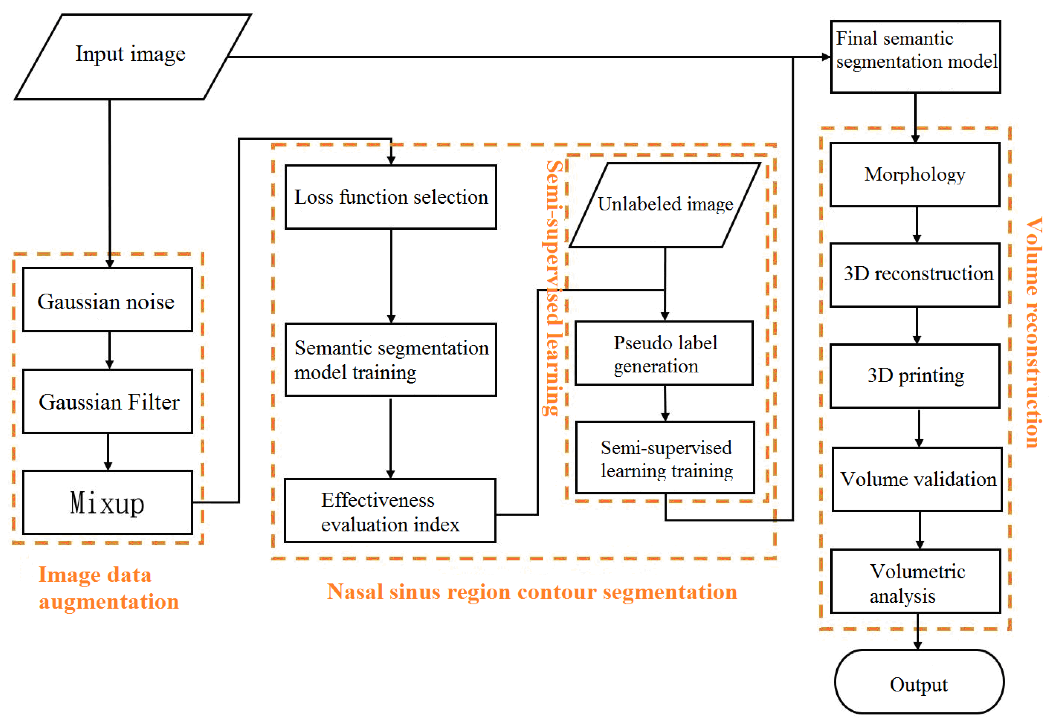
2. Methods and Experimental Data

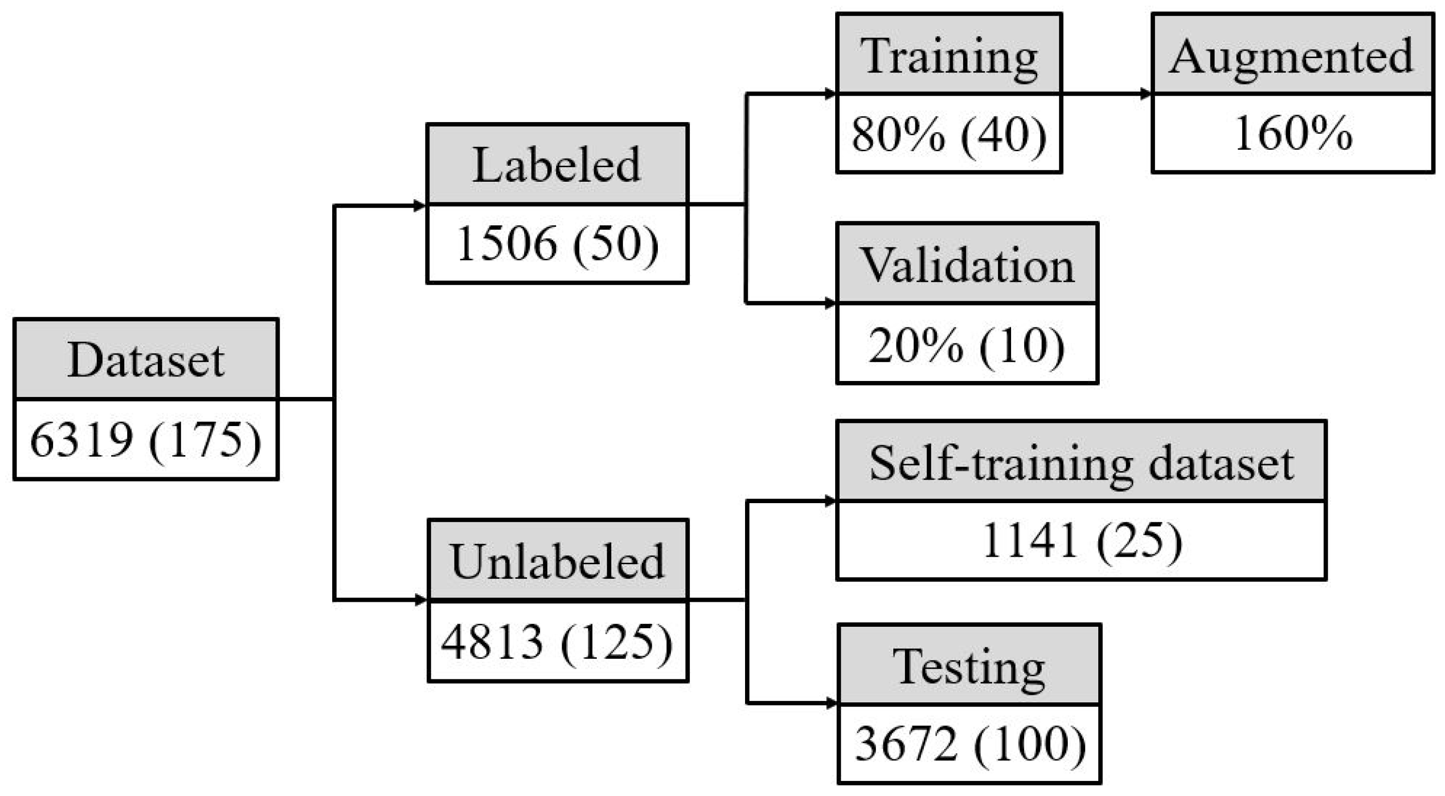
All subjects gave their informed consent for inclusion before they participated in the study. The study was conducted in accordance with the Declaration of Helsinki, and the protocol was approved by the Ethics Committee. (Project identification code: C202105070).

This study collected data from 175 patients, comprised of 117 male and 58 female subjects, who received head CT in Tri-Service General Hospital from 2018 to 2019 and aged from 16 to 80 years. The datasets were 512 × 512 gray level JPG images, out of which 50 datasets were images jointly labeled by doctors, as shown in Figure 1. These images labeled data contain five different nasal sinus regions, namely maxillary sinus, frontal sinus, anterior ethmoid sinus, posterior ethmoid sinus, and sphenoid sinus. The datasets were split into training and validation datasets by k-fold cross-validation. The 125 groups of unlabeled data were split into training datasets for semi-supervised learning and testing datasets for the doctors to evaluate effectiveness. The overall data allocation is shown in Figure 2.

The datasets are detailed below:

(1)

Training dataset: For the labeled dataset, the number of images was doubled by the data augmentation method. The basis of the gradient descent backpropagation algorithm was calculated by the input image and actual labeling result.

(2)

Validation dataset: For the labeled dataset, the gradient descent backpropagation algorithm was not calculated. Only the difference between labeling and prediction was calculated in each iteration to evaluate the effect of the model in every iteration.

(3)

Semi-supervised learning dataset: For the unlabeled dataset, a dataset for generating pseudo-labels after a model was trained.

(4)

Testing dataset: The unlabeled dataset was a dataset for evaluating effectiveness after model training was completed. Doctors would give evaluation scores to confirm model accuracy.

This study proposed a fully automatic system for accurate segmentation of five kinds of paranasal sinuses in the head CT (i.e., maxillary sinus, anterior ethmoid sinus, posterior ethmoid sinus, frontal sinus, and sphenoid sinus) and volume reconstruction 3D printing. The system flow includes image data augmentation, deep learning semantic segmentation, k-fold cross-validation, morphology, marching cube 3D reconstruction method, and 3D printing technique.

2.1. Image Data Augmentation

This study employed data augmentation to increase the object feature learning difficulty of the model, reduce the overfitting problem, and overcome data deficiencies to improve model effectiveness [24].

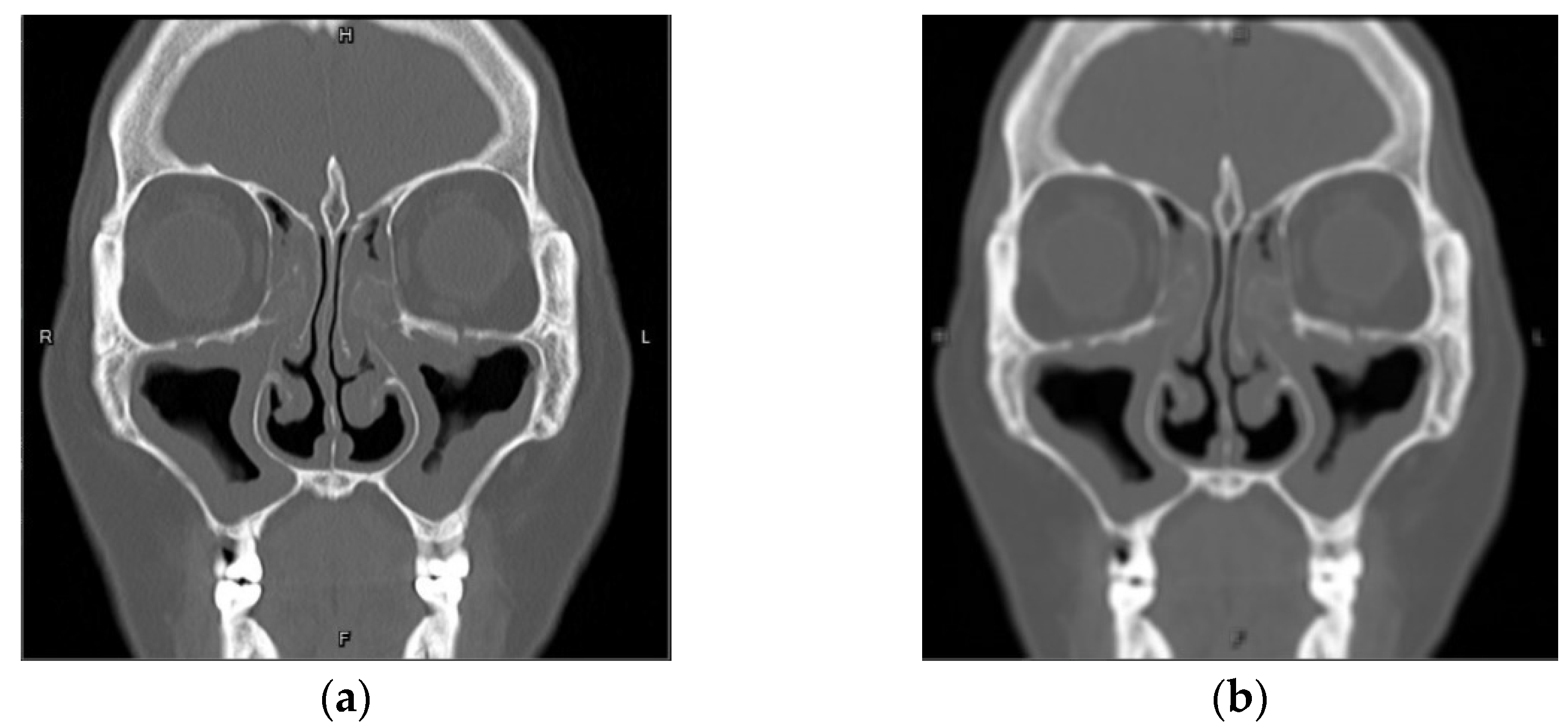
2.1.1. Gaussian Blur

Some images are blurred in the imaging process. In order to overcome the problem and make sufficient data for the training, data augmentation was adopted to obtain more fuzzy characteristics such as brightness, deblur, rotation, etc. in the model training process, thereby increasing the difficulty level of model training. The Gaussian blur [23] function distribution is expressed as Equation (1):

$$G(r)=\frac{1}{2\pi {\sigma }^2}{e}^{\frac{I{r}^2}{2\sigma }}$$

(1)

where γ is the blurred radius; σ is the standard deviation of normal distribution.

To equally allocate the weights of the images in two-dimensional space, the value of each pixel in the image is the weighted average of adjacent pixels. As the value of the original pixel has the maximum Gaussian distribution value, the weight is the largest. Further, the weight of the adjacent pixel decreases as the distance to the original pixel increases. Consequently, the edge effect is maintained better.

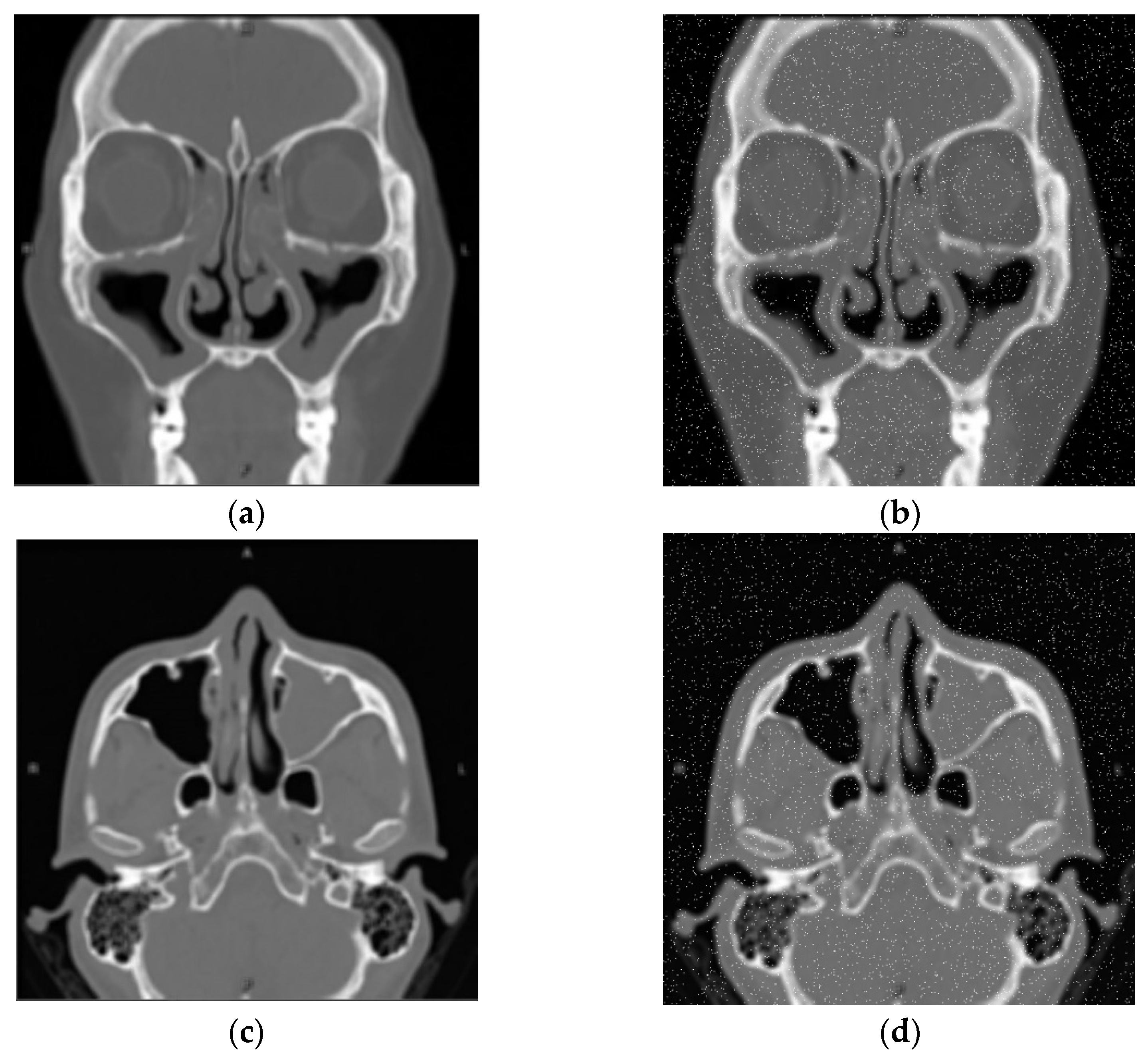
2.1.2. Gaussian Noise

As the CT imaging equipment employed in this study sometimes has image noise, the model adaptability can be enhanced by adding noise to the image data [25].

2.1.3. Mixup

This study adopted the Mixup Data Augmentation method [26] to combine the augmented data in order to accelerate the semantic segmentation model training process. Thus, the model learned images of different conditions, thereby learning different features, enhancing the model generalization effectiveness, and reducing the number of training iterations, defined as Equations (2) and (3):

$$\tilde{x}=\lambda x_i+(1-\lambda )x_j$$

(2)

$$\tilde{y}=\lambda y_i+(1-\lambda )y_j$$

(3)

where $x_i$ and $x_j$ represent two different input image samples; $y_i$ and $y_j$ represent the one-hot label encoding corresponding to the two different input image samples respectively; $\lambda$ is the ratio of the two image samples.

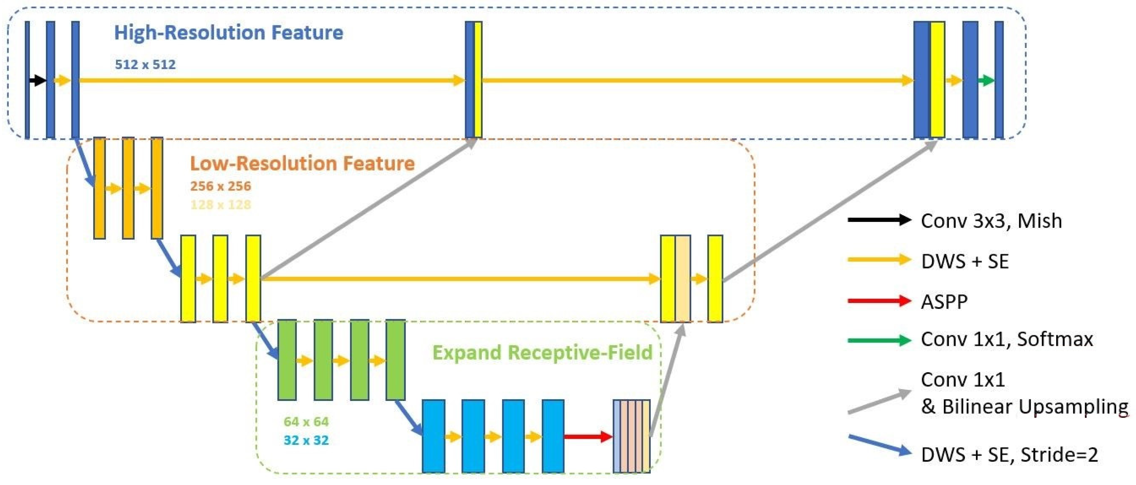
2.2. Semi-Supervised Learning

It was difficult to obtain the image segmentation data in this study and label all the obtained data. Thus, the unlabeled data were utilized using semi-supervised learning to enhance model effectiveness. Some labeled data were first employed in training, and then the trained model generated pseudo-labels for the unlabeled data to train the next model trained by a larger dataset.

In order to make the deep learning neural network model correctly learn the features of various nasal sinus regions—after the loss between neural network output layer value is correctly calculated—the neural network uses gradient descent and gradient to work out backpropagation to modify the neural network parameters. The gradient descent is expressed as Equation (4):

$$W_i=W_{i-1}-\gamma \frac{\partial L}{\partial W}$$

(4)

where $W$ is the weighting parameter; $\gamma$ is the learning rate; $L$ is the loss function.

$$V_i=\beta V_{i-1}-\gamma \frac{\partial L}{\partial W}$$

(5)

$$W_i=W_{i-1}-V_i$$

(6)

This study adopted the gradient descent with momentum to solve the local optimal solution when the gradient was 0 so that the parameters cannot be updated continuously, expressed as Equations (5) and (6): where $V$ is the directional velocity of momentum; $\beta$ is the momentum.

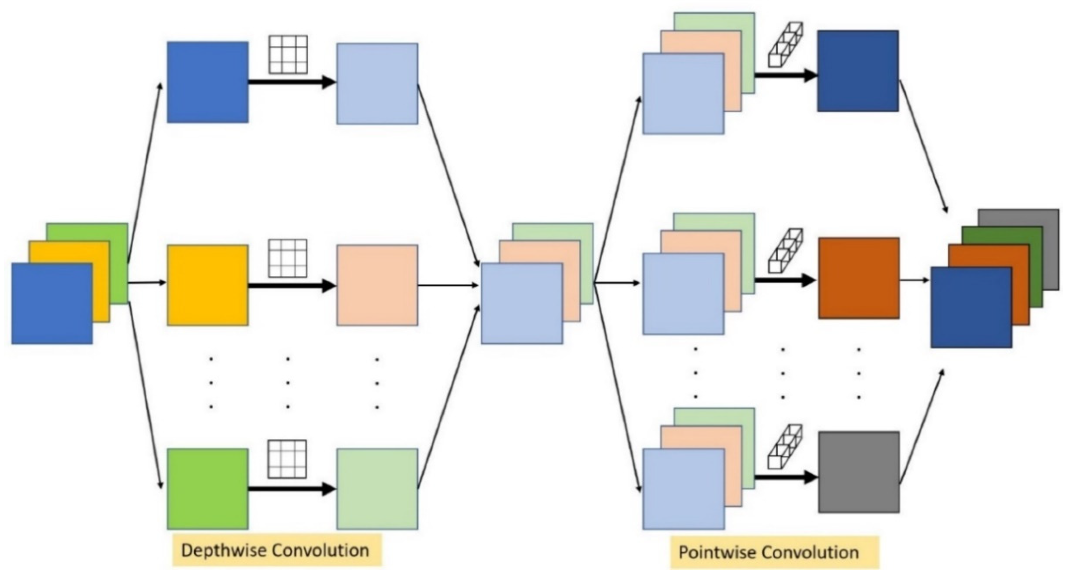
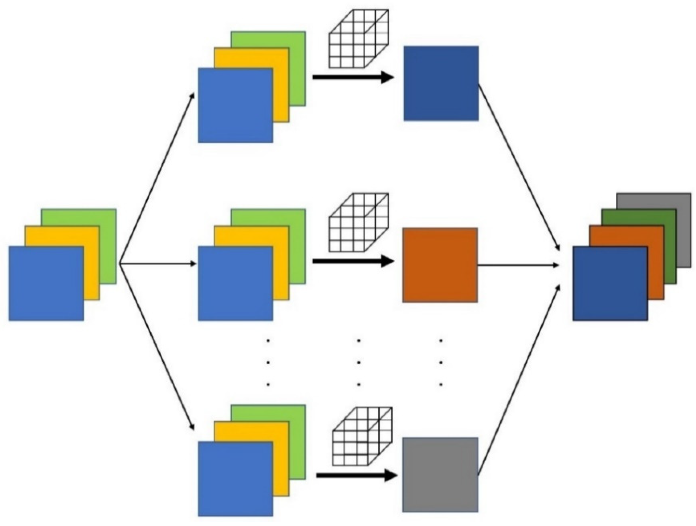
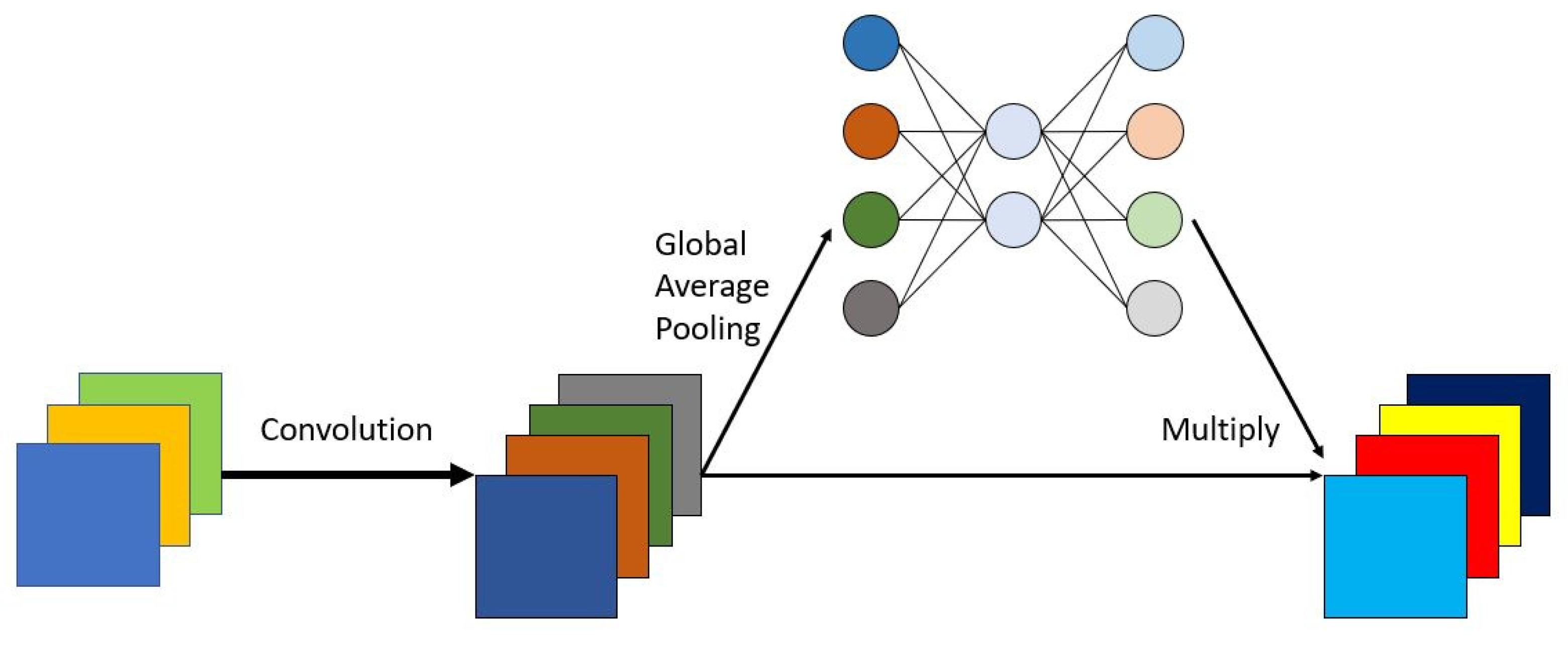
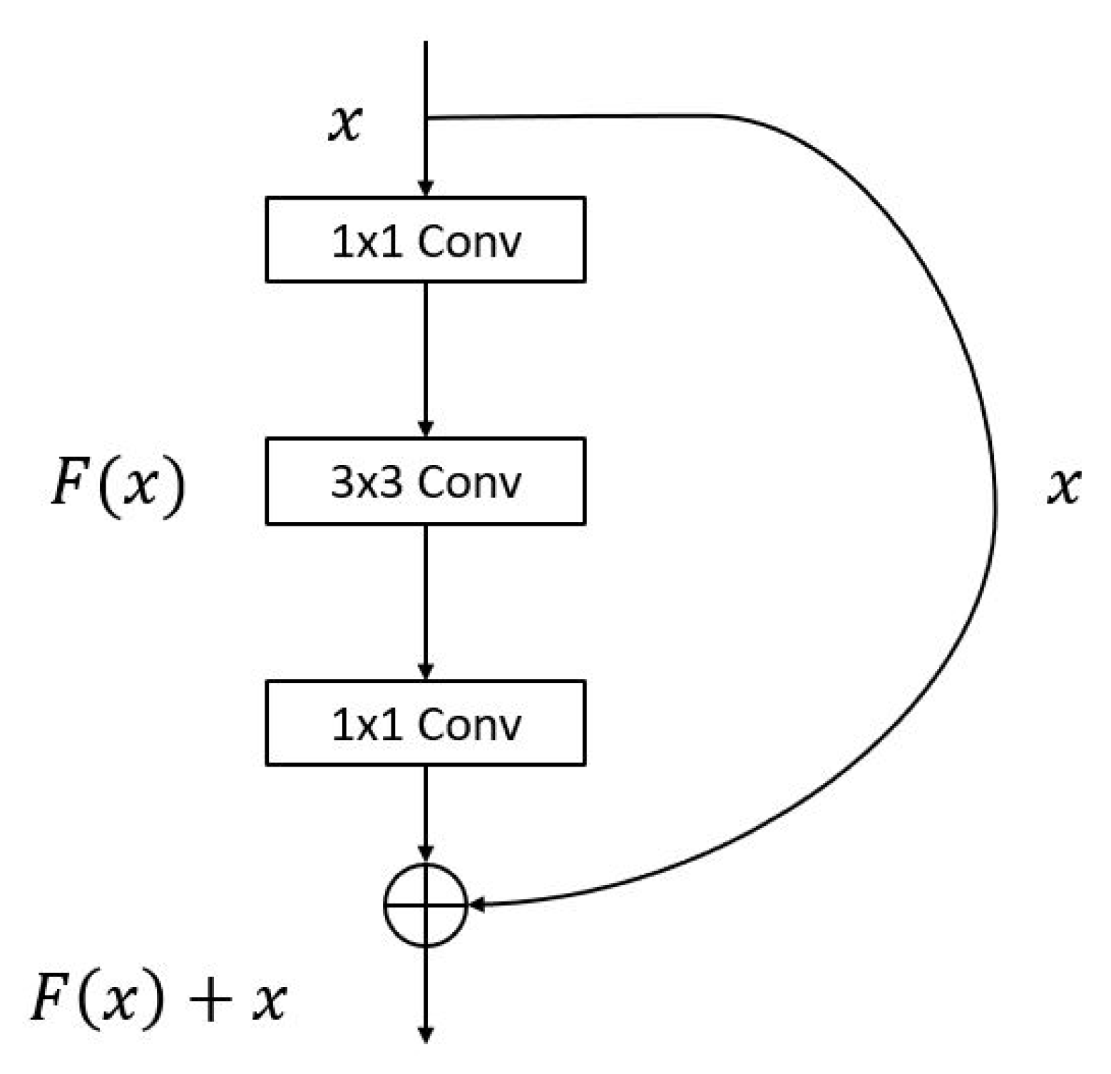
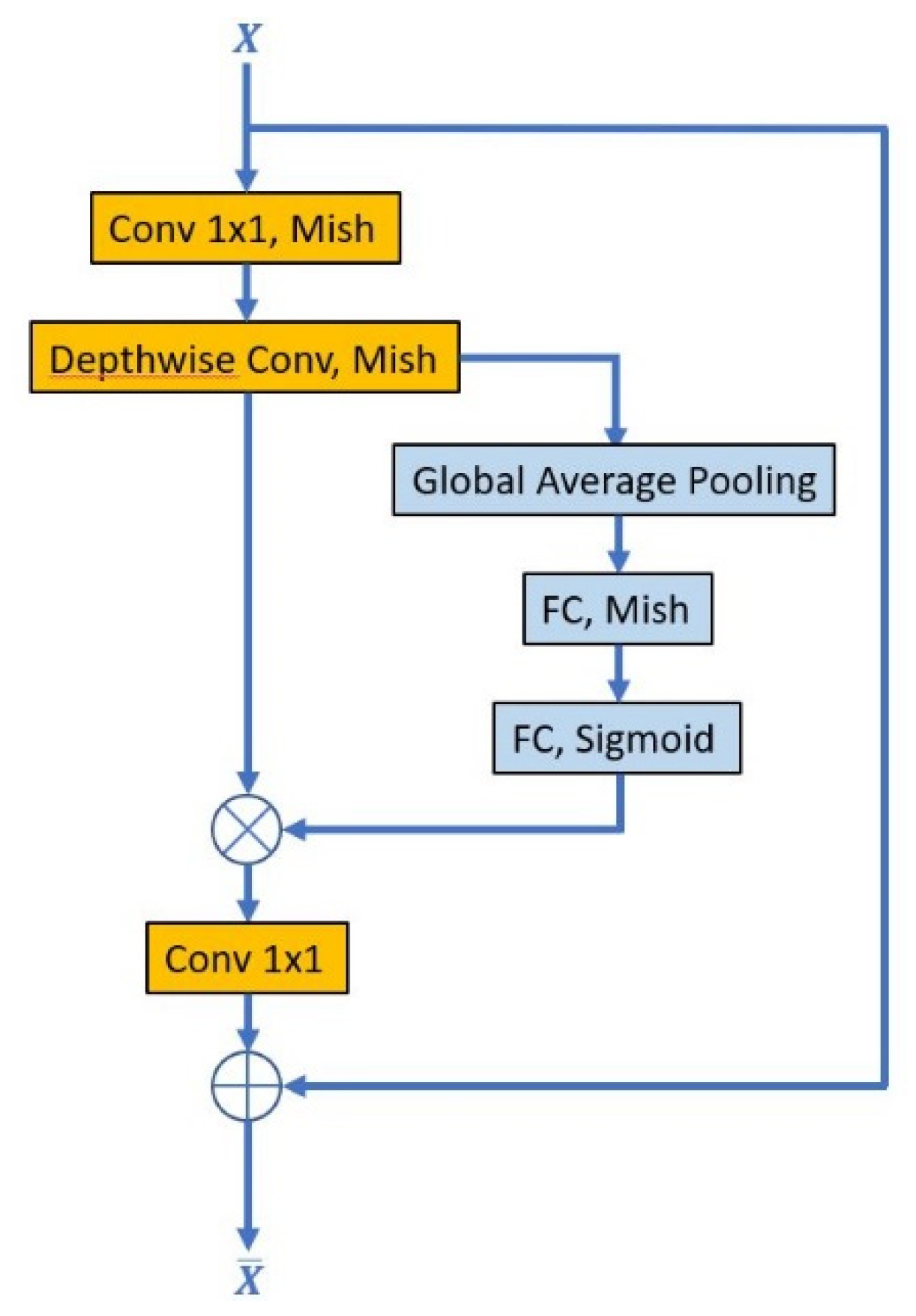
2.2.1. Convolution Layer

Many convolution layers were employed in the semantic segmentation to learn the feature contours of different paranasal sinuses [17]. The convolution layer is a set of parallel feature maps and learning features from an input image (e.g., line or edge) and is composed of sliding different convolution kernels on the input image or feature map, executing certain operations [19]. Additionally, in each slide position, a neuron corresponding product and summing operation is executed between the convolution kernel and input image project the information in the receptive field to a neuron in the feature map. The output size after convolution kernel operation of the input image or feature map is expressed as Equation (7):

$$N=\frac{(W-F+2P)}{S}+$$

(7)

where $N$ is the length-width size of the output feature map; $W$ is the length-width size of the input image or feature map; $P$ is the length-width size of convolution kernel; is the padding quantity to avoid ignoring the farthest edge of an image or feature map when the convolution kernel performs an operation. To keep output and input feature maps of equal size, P = 1 was used in this study and $S$ was employed as the step of convolution kernel (i.e., the sliding distance of each operation).

The deep learning model has numerous parameters that slow down or fail training and prediction in the hardware facilities with small memory. In order to increase the instruction cycle and reduce parameters, MobileNet [27] proposed depthwise separable convolution.

It has two steps. First, the depthwise convolution performs a convolution operation in a width of 1 for each width dimension in the upper feature map, as shown in Figure 3, which is different from the general convolution operation in Figure 4. The general convolution operation calculates all convolution kernels (width larger than 1) for each width dimension in the feature map. This method performs operations separately and uses 1 × 1 pointwise convolution to fuse these independent feature maps. Thus, the parameters can be reduced effectively when the convolution kernel is large, and the computing time can be shortened greatly [28]. Therefore, the general convolution was replaced by depthwise separable convolution in this study.

This study not only employed the depthwise separable convolution method to effectively reduce the amount of computation and lighten the weight of the architecture but also adopted squeeze-and-excitation networks [29] to train the influence weights among various feature maps. The important information of the feature map is further highlighted, as shown in Figure 5.

After the convolution operation, the squeeze-and-excitation network method employed global average pooling (GAP) to calculate the average value of different width dimensions and performed two fully connected layer neural networks to train the weights of different width dimensions. Finally, the learned weight was multiplied by the corresponding feature map width dimension, and the feature map was weighted, through which the importance of different width dimensions could be highlighted [30]. To make the output of the fully connected layer keep a normalized weight of 0~1, the Sigmoid function was used, expressed as Equation (8):

$$Sigmoid\left(x\right)=\frac{1}{1+e^{-x}}$$

(8)

Additionally, this study adopted the residual connection of residual neural network (ResNet) [31,32,33,34]; the training degradation problem in the very deep neural network was solved successfully, as shown in Figure 6.

$$x_L=x_l+{\displaystyle \sum _{i=1}^{L-1}F(x_i,W_i)}$$

(9)

$$\frac{\partial Loss}{\partial x_l}=\frac{\partial Loss}{\partial x_L}•\frac{\partial x_L}{\partial x_l}=\frac{\partial Loss}{\partial x_L}•\left(1+\frac{\partial }{\partial x_l}{\displaystyle \sum _{i=1}^{L-1}F(x_i,W_i)}\right)$$

(10)

where $x_l$ represents the input of the layer; $x_L$ represents the output of the layer. The effectiveness sometimes declines when the depth of the neural network is increased, leading to training degradation of the neural network. The residual connection guarantees at least identity mapping when computing gradient by backpropagation, and the gradient vanishing in multiple backpropagation processes is solved [35].

2.2.2. Activation Function

In this study, an activation function was added behind the convolution layer in the semantic segmentation model to increase the nonlinear characteristics of the model [19]. The common activation function in the convolutional neural network was rectified linear units (ReLU). The ReLU is more frequently used than the other activation functions because its functional operation is simple, where the instruction cycle of the neural network can be enhanced without a significant impact on the generalization accuracy of the model. Compared with the Sigmoid and Tanh functions used by conventional deep learning, the positive derivative of the ReLU function is 1. This special design alleviates the neural network gradient vanishing problem. Besides the ReLU function, the Mish function is extensively used in neural networks [36], expressed as Equation (11). When the input is a positive number, there is no limit value to the ReLU function. The main advantage is that the negative part is smoother than the ReLU function, which is different from the derivative 0 of ReLU in calculating the derivative by neural network gradient descent backpropagation. This activation function will not fail the update of corresponding neuron parameters.

$$Mish\left(x\right)=x•\tanh (\ln (1+e^x))$$

(11)

2.3. K-Fold Cross-Validation

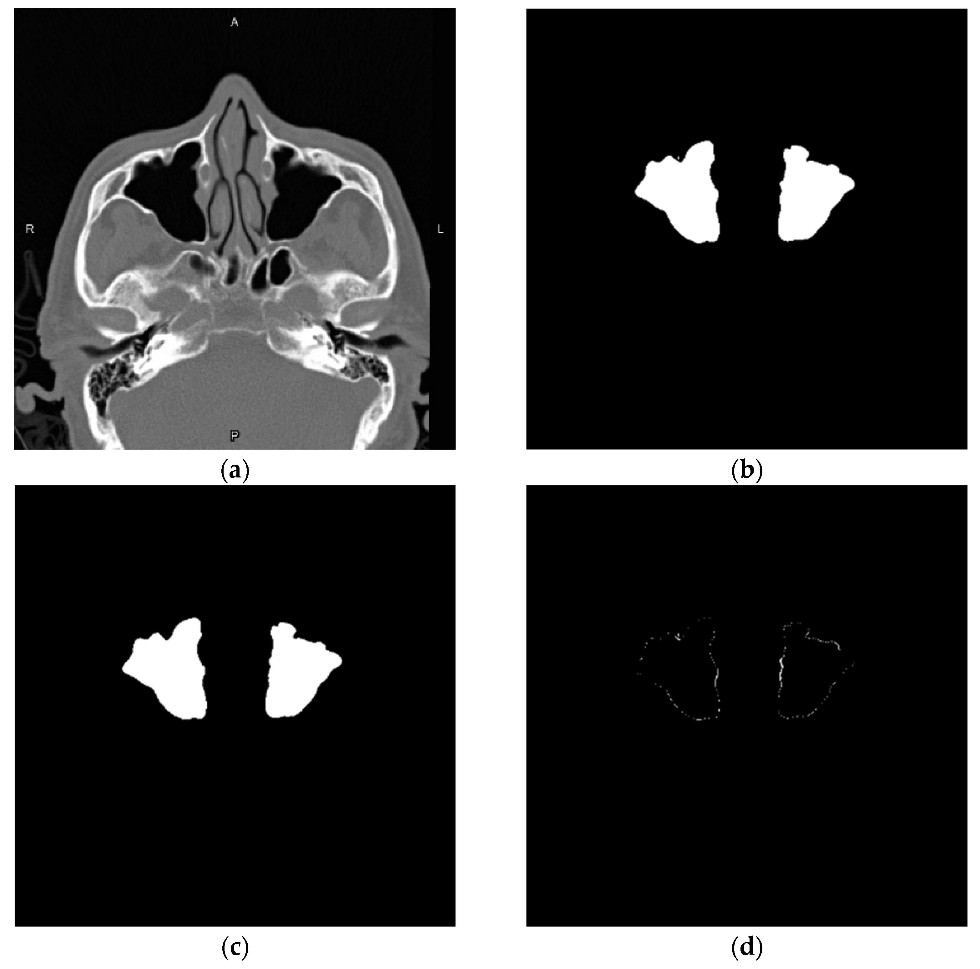
The K-fold cross-validation was employed to select the model for the next experiment. First, all the datasets were randomly divided into K equal parts; the data of the K − 1 part were used as a training dataset, and the residual part was used as a validation dataset. Afterward, one part was selected from the data, which was not used as a validation dataset. The data used as a validation dataset were added to the training dataset. Meanwhile, the K − 1 part remained for training and one part for validation. Then, the distribution was repeated until each part of the data had been used as a validation set, and the K iterative training and validations were performed. The single estimate could be obtained by averaging the K results. Further, similar to most deep learning methods, the data were randomly distributed into 80% training and 20% validation datasets. This study employed K = 5 to evaluate and select the optimal model [37].

2.4. Morphology

In this study, the region filter generated by the deep learning semantic segmentation model would be distorted by noise and texture so that the image might contain defects. This study also adopted morphology [38] to improve the filter. The shape of the structuring element was compared with the corresponding pixel neighborhood to generate dilation, erosion, opening, and closing results.

2.4.1. Erosion and Dilation

Erosion is the method that reduces the object image inward for several pixels. It has sets A and B, where B is the structuring element, A is eroded by B, as expressed in Equation (12).

The erosion shrinks or thins the object of the binary image and is most frequently used to remove the incoherent noise details in the binary image.

$$A\ominus B=\left\{z|{(B)}_z\subseteq A\right\}$$

(12)

In contrast to erosion, dilation dilates the boundary of the object image outwards for several pixels. It has sets A and B, where B is the structuring element, A is dilated by B, as expressed in Equation (13).

$$A\oplus B=\left\{z|[{\left(B\right)}_z\cap A]\subseteq A\right\}$$

(13)

The dilation expands the object of the binary image.

2.4.2. Opening

This study employed an opening to improve the left and right nasal sinus filters, which cannot be segmented. The opening made the object contour smoother, and the image was eroded before it was dilated. If Set A is opened by structuring element B, Set A is eroded by B, and B is dilated by the erosion result, as expressed in Equation (14):

$$A\circ B=(A\ominus B)\oplus B$$

(14)

2.4.3. Labeling

After the filters of different paranasal sinuses were predicted by the semantic segmentation model, this study adopted the labeling method to distinguish the left or right paranasal sinuses. The labeling of image processing meant that the adjacent pixels in the image were given the same label, and the connected pixels were regarded as the same region. The original image was divided into multiple regions based on this principle, and these regions were labeled to complete the labeling process [39].

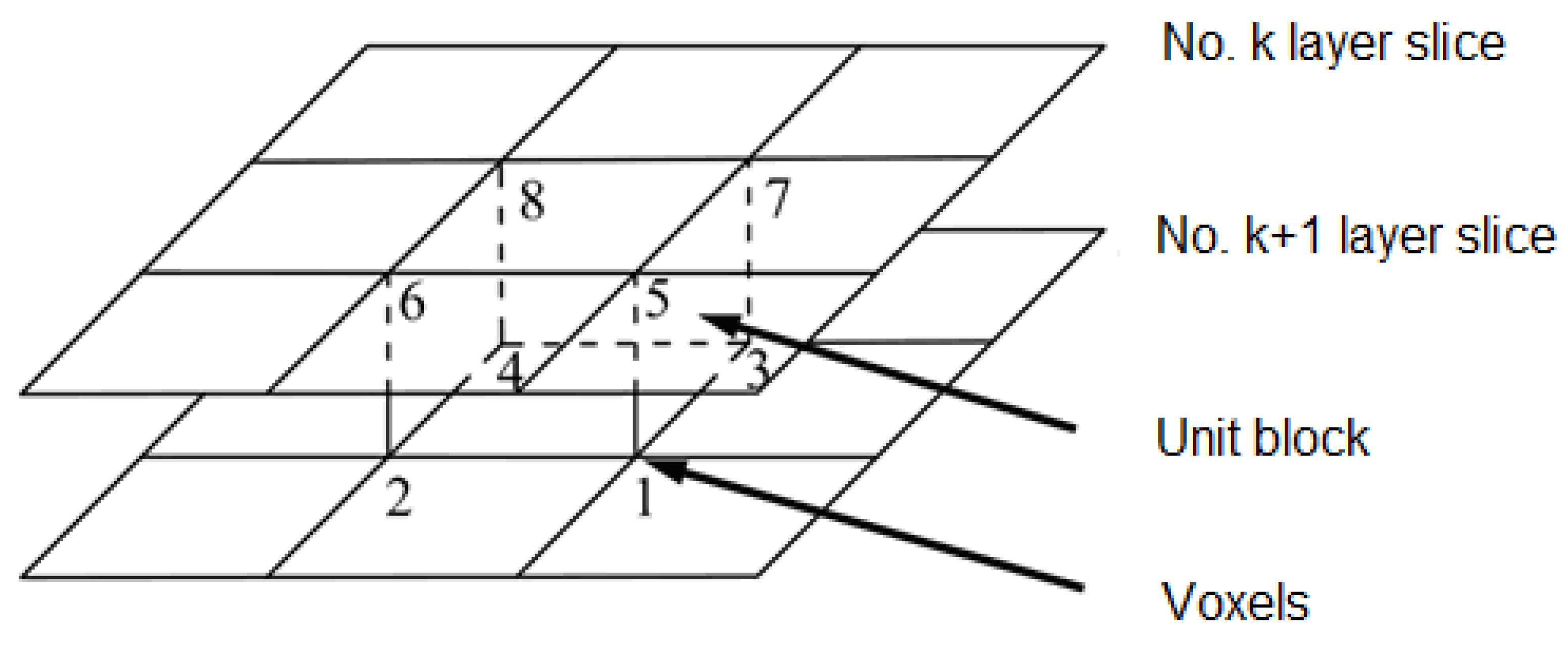
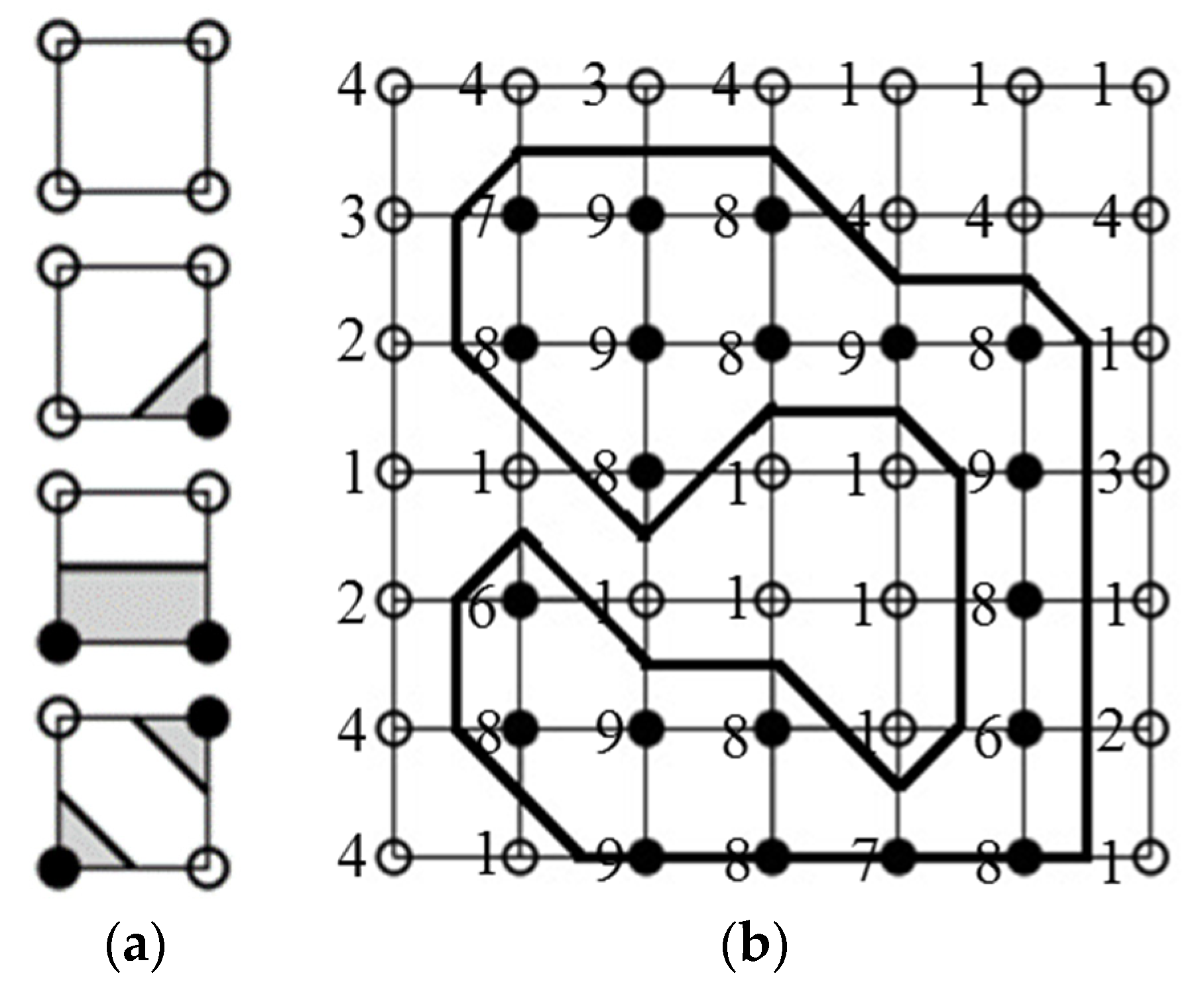
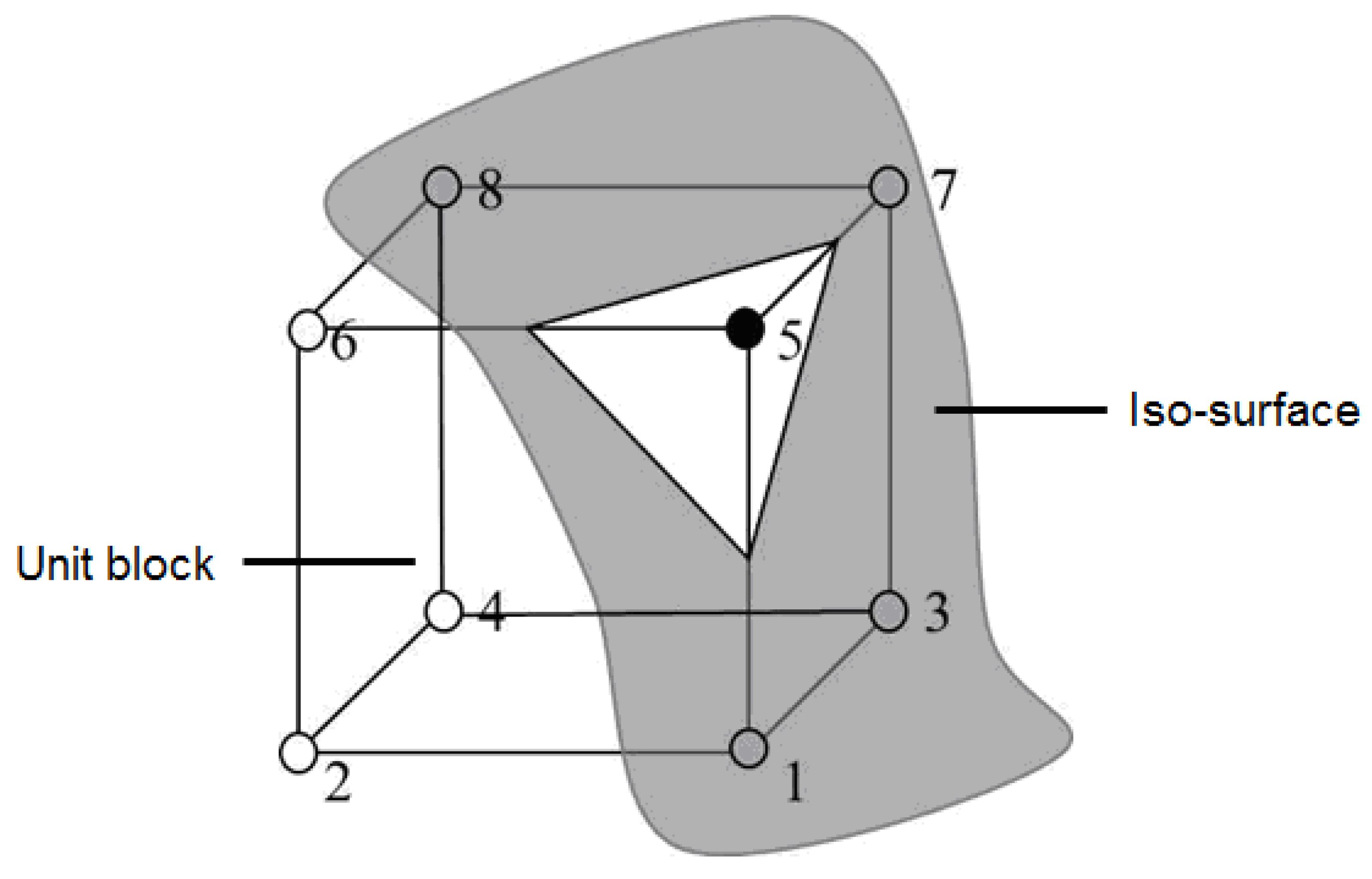
2.5. Marching Cube 3D Reconstruction

This study employed deep learning semantic segmentation to obtain the nasal sinus region filter and adopted the Marching Cube 3D reconstruction algorithm [40] to reconstruct the image of various nasal sinus regions. The Marching Cube algorithm assumes the data to be discrete rule data points in 3D space. Taking the samples in this study as an example, the length and width of each head CT image are 512 × 512; if there are 10 slices of nasal sinus regions, one continuous function collects samples 512, 512, and 10 times in x, y, and z directions, respectively, continuous nasal sinus region slice images can be obtained. Therefore, based on this characteristic, this study adopted the Marching Cube algorithm for filter as the method for reconstructing various nasal sinus regions. Its main procedure is described below.

First, the nasal sinus region slice images in the 2D image were filled with unit blocks of equal size. The unit block had eight vertices, which were defined as voxels, as shown in Figure 7. The eight vertices of the unit block comprised the pixels of two layers of head CT scan slices, and the pixels of each layer were connected in this way to define the continuous function $f\left(x_i,y_i,z_i\right)$ in the space.

After the continuous function in the space was defined, the iso-value was given, so that $f\left(x_i,y_i,z_i\right)=C$ constructed a surface, and the intersecting region of the unit block and surface was obtained. Before the intersecting region of the unit block and surface was obtained, the contour was described with 2D data, as shown in Figure 8 First, pixels greater than or equal to the iso-value were defined as black dots, while those smaller than the iso-value were white dots. As shown in Figure 8b, four adjacent pixels form a square, and each vertex has a chance to be black or white. The pattern symmetry has three combinations, as shown in Figure 8a. When four vertices were all black or all white, it implies that the square was inside or outside the isocontour, and the opposite isocontour must have passed through a square with black dots at one end and white dots at the other end. For convenient demonstration, the pixels were represented only by 1~10, the iso-value was 6, and the isocontour was generated, as shown in Figure 8b.

The 2D data were extended into the 3D dataset to find the iso-surface, the original 2D square was changed into a 3D unit block, and the four vertices were changed into eight vertices of voxels. First, the iso-value was given; if the eight voxels of the unit block were greater than or equal to the iso-value, they were inside the iso-surface, otherwise outside. Similar to 2D data, the iso-surface would have passed through a unit block with one end smaller than the iso-value and the other end greater than or equal to the iso-value. If all the voxels were larger than or smaller than the iso-value, the iso-surface would not pass through the unit block, as shown in Figure 9.

Subsequently, the unit block was processed by line-search. As the eight voxels in the unit block were inside or outside the iso-surface, there were 28 combinations, which could be reduced to 15 according to the symmetric property of the method. The unit block illustration described the process of generating triangular iso-surface in the unit block.

Whether the iso-surface passes through the unit block was analyzed, the intersection point at the edge was obtained by linear interpolation, and the triangular iso-surface was generated online. The triangular facets of each unit block were connected to form a triangular mesh for 3D reconstruction.

2.6. Implementation Challenges

CT images are an important element to find sinusitis disease using the deep learning method. If the CT images are not good enough and labeled not properly then the deep learning method fails to learn. Therefore, acquiring CT images during data collection, the clinician must be careful. After collecting the data, the next challenge is to decide data augmentation technique. If the data augmentation doesn’t meet the requirement based on CT images and based deep learning network, then also model fails to perform well. Therefore, the data augmentation technique must be done carefully and reasonably. Tuning hyperparameters is also a challenge; however, this can be overcome by training the model with a greater number of epochs and filters in the network.

3. Results

This experiment was divided into four major parts. Part 1 is the image data augmentation. Part 2 is the nasal sinus region segmentation, using different deep learning semantic segmentation models to train the datasets collected in this experiment. Part 3 employs the unlabeled image data for semi-supervised learning training, and the last part exhibits the volume reconstruction and analysis. The experimental system flow chart is shown in Figure 10.

3.1. Image Data Augmentation

This study adopted the image data augmentation technology, making finite data generate more equivalent data to augment the training dataset. The data deficiencies were overcome, and the data augmentation method could increase the difficulty of the model for object features. In addition, the overfitting problem can be reduced [41], improving model effectiveness.

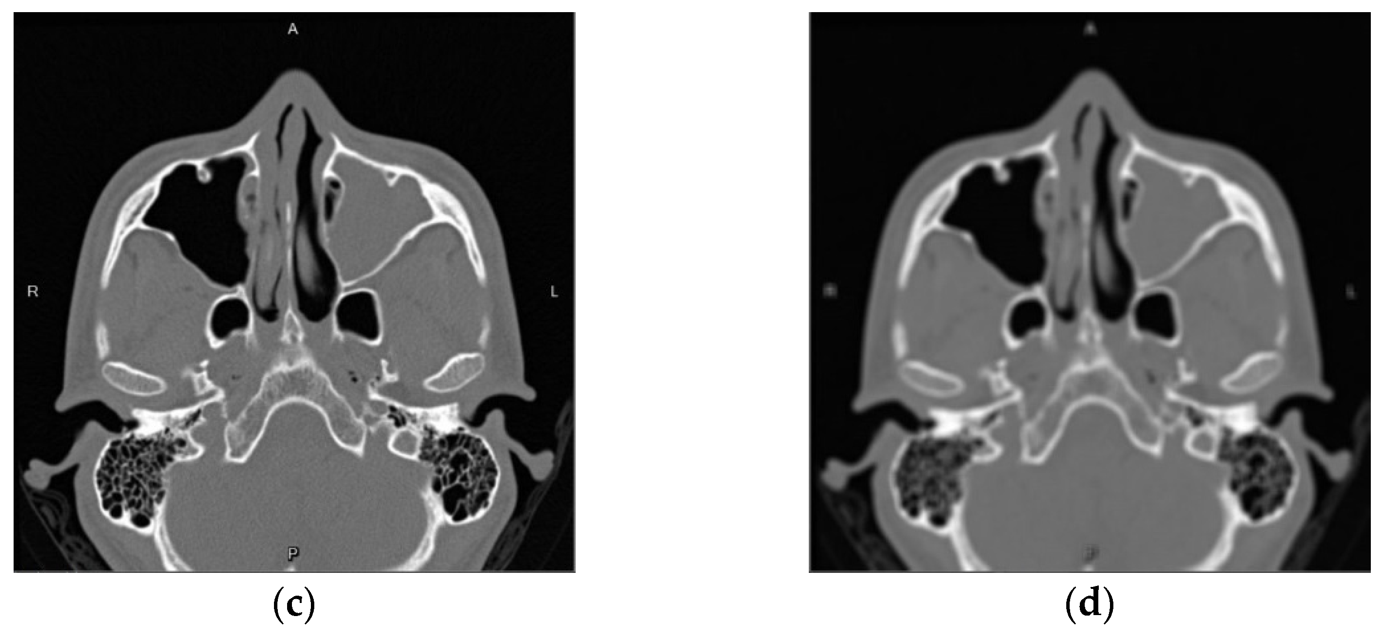
3.1.1. Gaussian Blur

The imaging blurred image samples often occur in the research on experimental data samples. Partial images were also blurred in the course of imaging in this study. Thus, the blurred image samples were intentionally made using Gaussian blur, and more fuzzy characteristics were obtained in the model training process, as shown in Figure 11.

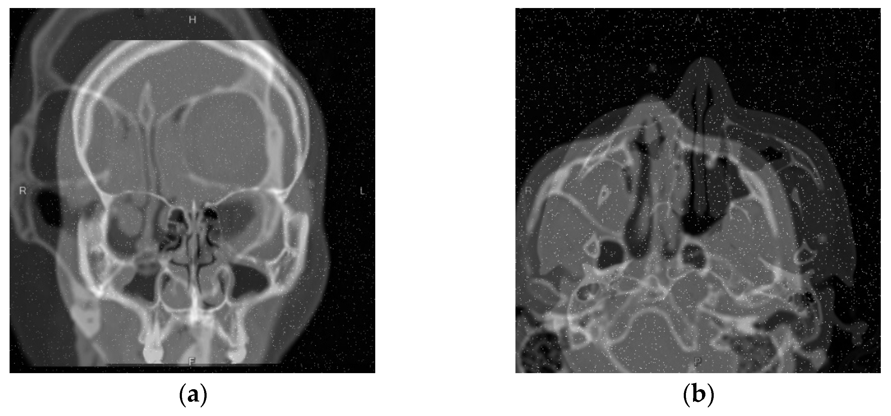
3.1.2. Gaussian Noise

After the CT image was blurred, the Gaussian noise was employed for the Gaussian distribution of the original blurred image, and the training difficulty of the semantic segmentation neural network model was further increased. Increasing noise in the input image is similar to using the Dropout method to reduce overfitting, as shown in Figure 12.

3.1.3. Mixup

Besides the two data augmentation methods of Gaussian blur and Gaussian noise, some common data augmentation methods for deep learning image recognition were adopted, such as random rotation, mirror reflection, contrast, and brightness control. Finally, a randomly selected original training dataset input image and another augmented similar data were combined using the Mixup method, forming a new data augmentation training dataset. The result is shown in Figure 13. The Mixup data refers to the superimposition of the original image and it is one of the augmented images. Figure 13a,b are the Mixup images which has original and random rotation augmented images in them. The purpose of this type of data is to feed images with more noise to the model for better identification.

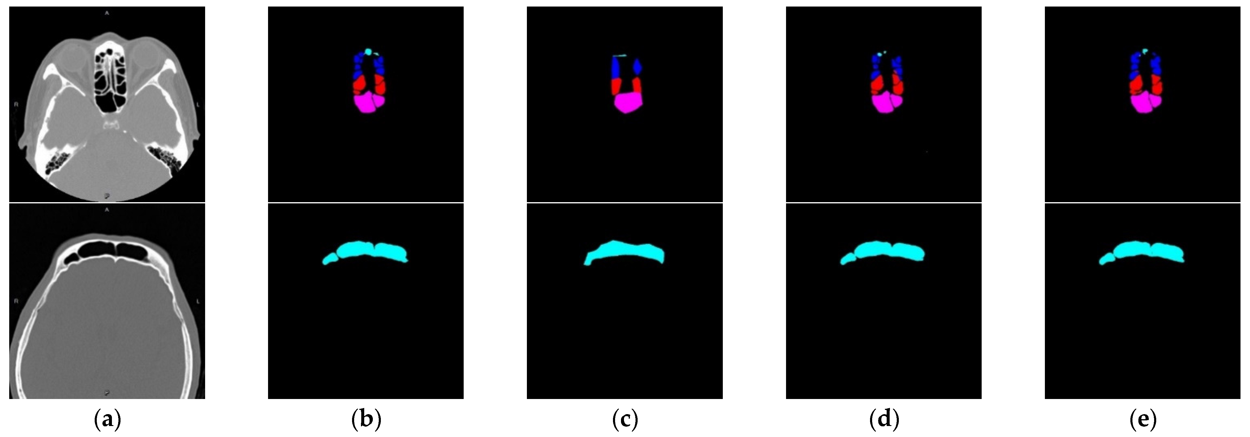
3.2. Nasal Sinus Region Segmentation

To calculate the volume of each nasal sinus, the system should segment all kinds of nasal sinus contour regions for subsequent calculation. This section will detail the result of deep learning semantic segmentation used in this procedure.

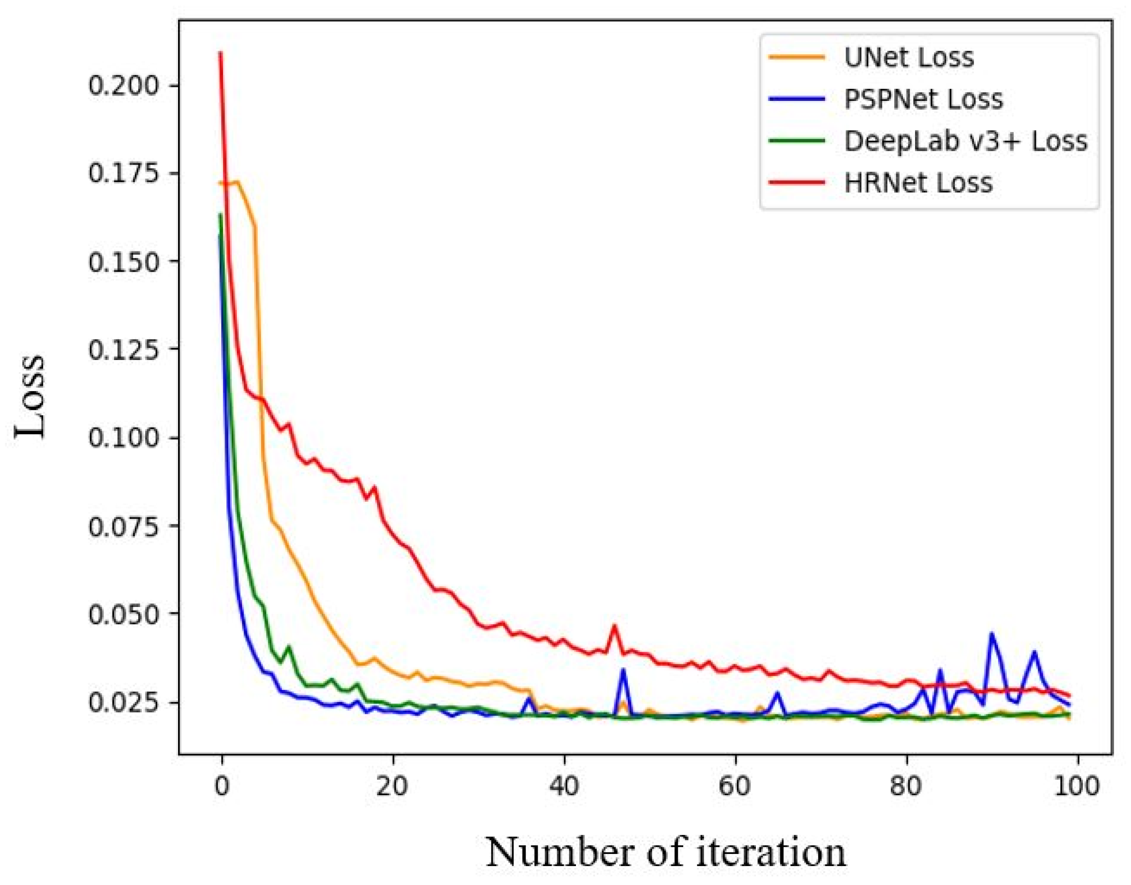
3.2.1. Loss Function Selection

The selection of the loss function is significant in optimizing the semantic segmentation model to accurately classify the paranasal sinuses of various pixels. For semi-supervised learning of probable pseudo labels, this study used Cross − Entropy as a loss function method.

$$Cross-Entropy={\displaystyle \sum _{c=1}^C{\displaystyle \sum _{i=1}^n-y_{c,i}\log (p_{c,i})}}$$

(15)

where $C$ is the number of classes; $n$ is the number of data; $y_{c,i}$ is the actual answer; $p_{c,i}$ is the predicted probability of No. $i$ data belonging to class $C$. The closer the predicted probability is to the actual answer, the closer the value is to 0. On the contrary, if the predicted probability is quite different from the actual answer, the value is close to 1. In order to calculate the class probability of each pixel, the softmax is used in the output layer, expressed as Equation (16). Since there are multi-class classifications involved in the model, softmax is used to classify the output with the probability of each class [42].

$$Softmax=\frac{e^{z_i}}{{\displaystyle \sum _{i=1}^K{e}^{z_i}}}$$

(16)

where $Z_i$ is the output of No. $i$ output layer.

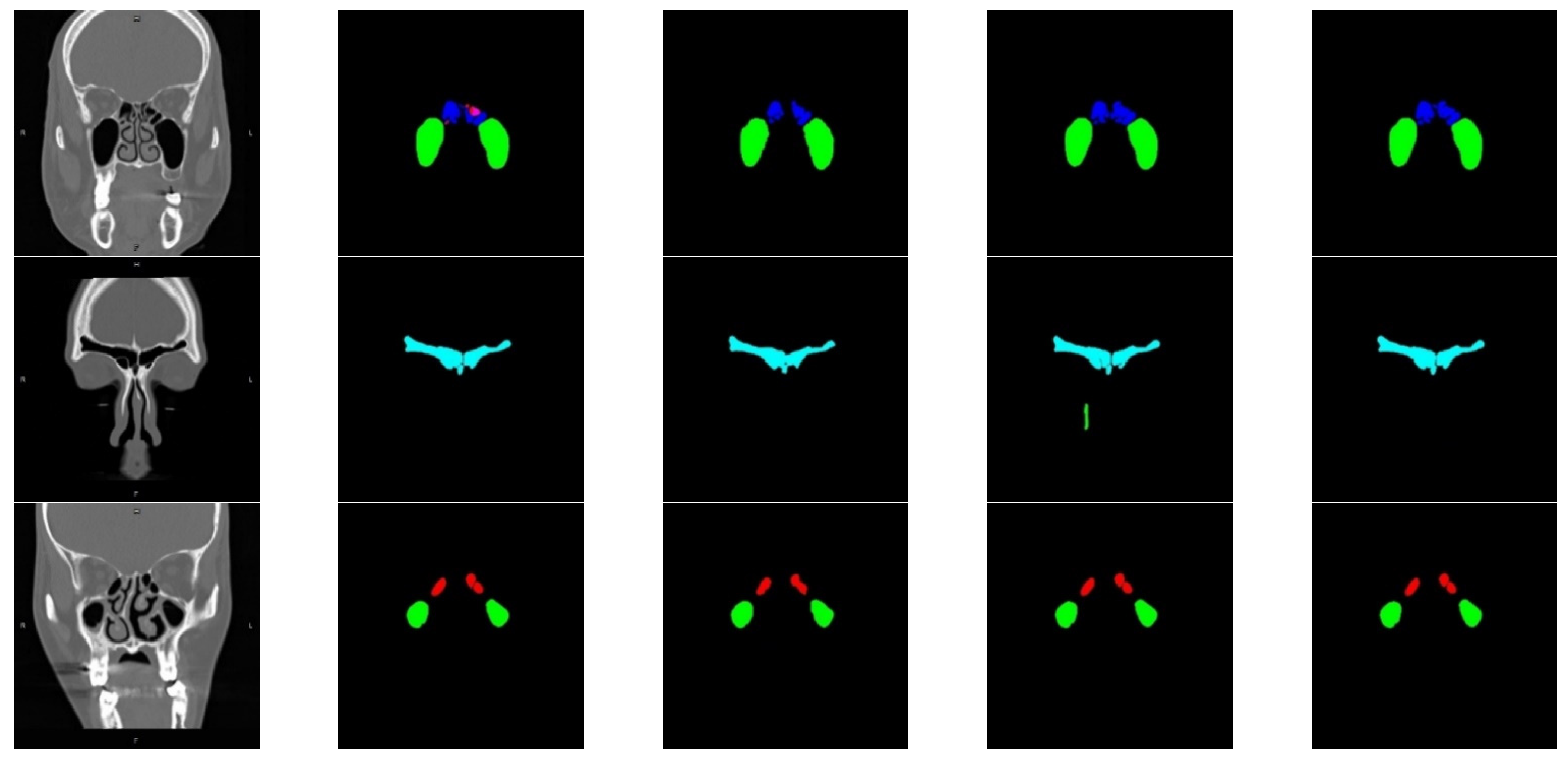
3.2.2. Semantic Segmentation Model Training

This study employed various famous deep learning semantic segmentation models, including UNet [43], PSPNet [44], DeepLab v3+ [45], and HRNet [46] to train and iterate the datasets 100 times. After preliminary training of these semantic segmentation models, the losses have converged. UNet has a minimum loss, followed by DeepLab v3+, shown in Figure 14. The training result prediction images are shown in Figure 15, where green is the maxillary sinus; blue is the anterior ethmoid sinus; red is the posterior ethmoid sinus; cyan is the frontal sinus; pink is the sphenoid sinus.

Besides basic convolution operation, the depthwise separable convolution, squeeze-and-excitation networks, and residual connection were used in this study’s deep learning semantic segmentation model. The entire model was divided into three main stages: high-resolution feature, low-resolution feature, and expanded receptive field feature, as shown in Figure 16 and Figure 17. The expanded receptive field feature part employed dilated convolution and Atrous Spatial Pyramid Pooling to further enhance the receptive field of the model, which was integrated with the peripheral information of the nasal sinus region. The low-resolution feature was combined with the expanded receptive field feature information and combined with a high-resolution feature, respectively. Different detail features of different feature map scales were fused to make the nasal sinus contour more legible and complete. The up sampling adopted bilinear difference to guarantee a larger receptive field and maintain clear contour detail.

The common ReLU of the first fully connected layer activation function in the squeeze-and-excitation was changed to the latest activation function Mish [36]. The Mish activation function has been proven more accurate in other experiments [47]. The first 1 × 1 convolution dilated the feature map. The feature was extracted using depthwise separable convolution and multiplied by squeeze-and-excitation to obtain the weighted feature map. Then, a linear 1 × 1 convolution was adopted to compress the feature map, which was added by residual connection to deliver the neural network gradient to the next layer.

3.2.3. Effectiveness Evaluation Indexes

This study employed Pixel Accuracy, Mean Intersection-Over-Union, and Dice Coefficient as evaluation indexes.

(1)

Pixel Accuracy (PA):

Pixel Accuracy is the correct rate of all pixels in the image.

(2)

Mean Intersection-Over-Union (MIoU)

$$\frac{A\cap B}{A\cup B}=\frac{TP}{(TP+FP+FN)}$$

(17)

The IoU is the Intersection over Union. When the predicted image and the labeled image are not intersecting, the output is 0. On the contrary, when the predicted image and the labeled image are fully intersecting, the output is 1. The Mean IoU was adopted for the multi-class segmentation of images in this study.

(3)

Dice Coefficient

The Dice Coefficient is similar to IoU, a double intersection of pixels of the predicted image and the labeled image.

$$\frac{2\left|A\cap B\right|}{\left|A\right|+\left|B\right|}=\frac{2\ast TP}{\left(TP+FN\right)+(TP+FP)}$$

(18)

3.3. Semi-Supervised Learning

After the semantic segmentation model training was completed, this study employed a semi-supervised learning training method for further training [48] to further optimize the semantic segmentation model. For the data in this study, the data volume of 6319 CT images was adequate; labeling all these image data to train the model would take a lot of time.

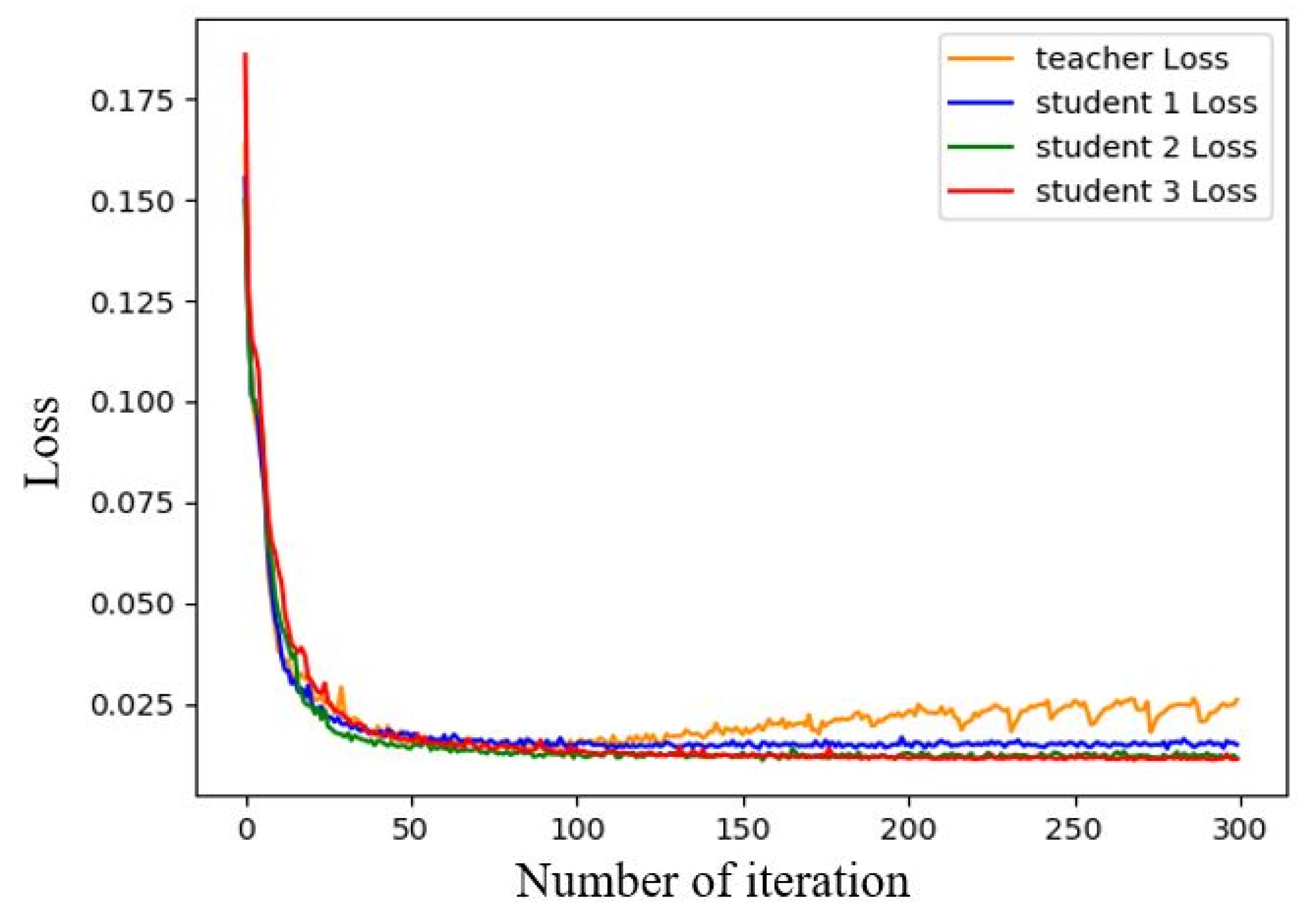
3.3.1. Pseudo Label Generation

Besides 1506 labeled image data, 1141 unlabeled image data were prepared for semi-supervised learning. The pseudo label should be generated for these unlabeled image data before training. The CT images were imported into the trained semantic segmentation model so that the semantic segmentation model could predict the probability class of various paranasal sinuses of various pixels through softmax. In predicting the contour of the maxillary sinus region, as shown in Figure 18, the probability higher than a value was adopted as new label data through a predicted self-confidence threshold. This threshold is the optimum threshold selected by calculating the maximum Dice score of the validation dataset, as shown in

Table 1. Optimum threshold table.

Self-Confidence Threshold	Dice
0.3	90.79%
0.4	90.79%
0.5	90.79%
0.6	90.81%
0.7	90.83%
0.8	90.67%
0.9	90.16%

.

Figure 18d is derived from subtracting the pseudo label image from the predicted image, showing that the self-confidence threshold can filter the pixels without the confidence of the semantic segmentation model [49] to increase the Dice score of the corresponding validation dataset.

3.3.2. Semi-Supervised Learning Results

After the semantic segmentation model generated the pseudo label, the former could be trained for semi-supervised learning with labeled data. Finally, the difference between the minimum losses of the third and second training is only 0.0003, as shown in

Table 2. Semi-supervised learning training table.

Frequency of Repetitive Training	Minimum Loss
0	0.0211
1	0.0192
2	0.0175
3	0.0172

.

In the semi-supervised learning training process, more data augmentation noise was added to the unlabeled image to avoid overfitting in the semantic segmentation model. Each feature map of the low-resolution feature and the expanded receptive field was normalized using dropout [50]. The dropout was employed in the part of a high-resolution feature in the experimental process. As the Gaussian noise had been added in the CT image, the features of various nasal sinus region contours of model training would be damaged. Further, the convolution kernel width was modified to double VGG16 of the previous width whenever a depthwise separable convolution kernel in step size of 2 was passed by [51]. The new neural network feature map width trained three times was increased from 8 to 1.5, 2, and 2 times to train the features of more dimensions in each training process. The training result is shown in Figure 19, where the teacher represents the original semantic segmentation model, and the student represents the frequency of repetitive semi-supervised learning training.

3.4. Volume Reconstruction

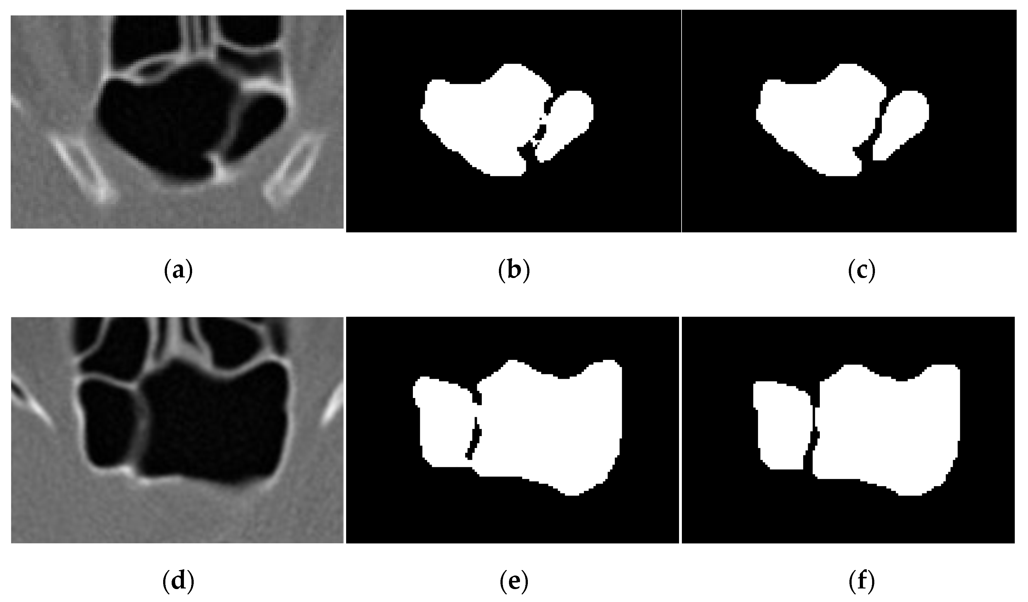
After the contours of five kinds of nasal sinus regions were predicted by the semantic segmentation model to further clarify the 3D nasal sinus contour to provide clinical reference observation for doctors, the morphology and 3D reconstruction were adopted in this study for processing.

3.4.1. Morphology

In terms of the contours of nasal sinus regions predicted by the semantic segmentation model, left or right paranasal sinuses cannot be recognized successfully because a small part of paranasal sinuses does not have an apparent edge. Therefore, this study employed the opening method of morphology and subsequently adopted the connection representation of morphology to distinguish left and right paranasal sinuses. The result is shown in Figure 20 and Figure 21.

The left and right paranasal sinuses can be distinguished effectively using the opening method. After the left and right paranasal sinuses were recognized using labeling and the air section (black) and mucosa inflammation region (gray) under the nasal sinus region were segmented by the threshold, the severity of sinus mucosa inflammation in the CT image could be clarified directly to calculate the mucosa inflammation condition of different paranasal sinuses. The final segmentation is shown in Figure 22, and the system execution output is shown in Figure 23.

3.4.2. 3D Reconstruction

Furthermore, this study employed the Marching Cube algorithm to reconstruct the image of paranasal sinuses in order to clearly observe the shape or the mucosa inflammation condition of paranasal sinuses. First, the obtained 2D nasal sinus images were overlapped to form 3D matrix data. The unit block was added to each layer of the 2D matrix, and the voxels were defined to evaluate whether or not the voxels in each unit block were larger than the iso-value. Subsequently, the triangular mesh in each unit block was established. Finally, all the triangular structures were connected to reconstruct the image, as shown in Figure 24. The maxillary sinus, ethmoid sinus, frontal sinus, and sphenoid sinus were reconstructed, with the gold being the right nasal sinus, the blue being the left nasal sinus, and the red arrow being the orientation of the face. The sinus mucosa inflammation proportions are shown in Figure 25, with the gold being the right nasal sinus, the blue being the left nasal sinus, the gray being the uninflamed region, and the red arrow is the orientation of the face. Figure 26 shows the 3D reconstruction image of the overall paranasal sinuses.

4. Discussion

Normal sinuses appear black in CT scan images because the sinuses are filled with air, and as long as there are symptoms of gray mucosal inflammation in the sinuses, it can be called sinusitis. Therefore, CT scans can evaluate the scope of sinus inflammation, severity and help diagnose the assessment and decide on the treatment of the disease [1]. The Lund-Mackay grading system is a method used by physicians to observe the severity of sinusitis using computed tomography, so it can be known that if the Lund-Mackay score is 0, it means that there is no sinusitis. However, if physicians are required to view continuous two-dimensional image CT images, they cannot accurately know how serious it is. Garneau et al. [3] used a grading system that calculated the proportion of mucosal inflammation as a standard for evaluating the severity of sinusitis. The study achieved better results than the general Lund-Mackay score. However, it takes more than an hour to manually select various sinus contours in all computed tomography slice images. Compared with the grading system that calculates the proportion of sinus mucosal inflammation in the same system and the experiment, there is a big difference of only 9.7 s. Therefore, the study provides a more rapid, objective, and accurate tool for assessing the severity of sinusitis, as the gold standard for measuring the severity of sinusitis in the future.

Despite the high incidence of chronic rhinosinusitis, the optimal strategy for treating chronic rhinosinusitis has so far been uncertain, so there is no specific relationship between the degree of sinus inflammation and the decision to perform sinus surgery or use of medication. In the Lund-Mackay study [52], it was also stated that the score is only a method of assessing and quantifying the degree of inflammation in sinusitis, so as a study of clinical criteria, there is no absolute score threshold for sinusitis surgery. Patients improved better after surgery, but there was no certain score threshold to tell patients how much they must have surgery. Therefore, in order to better recommend whether patients with chronic rhinosinusitis should undergo surgery, this study traced the past medical records of chronic rhinosinusitis and calculated a grading system for the proportion of sinus mucosal inflammation as a recommendation index for surgery. Through the Youden index and the optimal threshold to assess whether the need for surgery can be effectively diagnosed. The optimal threshold is 6.92 when the appropriate score is 99.67%, 90.79%, and 88.75% for the PA, Dice, and mIOU respectively, which proves that the system can provide good surgical advice to physicians.

The three effectiveness evaluation indexes were worked out according to the trained semantic segmentation models. The result is shown in

Table 3. Semantic segmentation model effectiveness comparison table.

Method	PA	Dice	mIOU
UNet	99.56%	89.68%	87.83%
PSPNet	99.31%	87.52%	85.78%
HRNet	99.12%	86.68%	83.02%
DeepLab v3+	99.55%	89.64%	87.69%
Our + MobilenNet [53]	99.62%	90.41%	88.53%
Our + ResNet50 [31]	99.63%	90.47%	88.57%
Our + ResNet101 [31]	99.63%	90.51%	88.58%
Our + ResNext50 [31]	99.63%	90.49%	88.58%
Our + ResNext101 [31]	99.64%	90.55%	88.59%
Our + Inception [56]	99.65%	90.57%	88.59%
Our + DWS + SE	99.67%	90.79%	88.75%

. UNet has the best effect, followed by DeepLab v3+, PSPNet, and HRNet. The semantic segmentation models used in this study were compared using different prominent convolutional neural network backbone methods, such as MobileNet [53], ResNet [31], ResNext [27], and Inception [54,55,56].

According to the experimental results in

Table 4. Semi-supervised learning effectiveness comparison table.

Method	PA	Dice	mIOU
UNet	99.56%	89.68%	87.83%
Our	99.67%	90.79%	88.75%
Our + Semi-supervised learning	99.75%	91.57%	89.43%

, the nasal sinus region segmentation accuracy can be enhanced greatly by combining the semantic segmentation model with semi-supervised learning training. Besides accuracy, the difference from the UNet computing time was worked out. The time for predicting each of the 100 head CT images is shown in

Table 5. Validation dataset performance comparison of various models.

	Computer Equipment 1	Computer Equipment 2
CPU	Intel®Core™ i5-7300	Intel®Xeon® Silver-4110
Memory	16GB DDR4	64GB DDR4
Graphic card	NVIDIA GTX1050 4 GB	NVIDIA Quadro GP100 16 GB
UNet prediction time	0.076 s	0.057 s
Prediction time of this model	0.082 s	0.062 s

. The nasal sinus segmentation effectiveness has enhanced a lot.

In order to analyze the predicted result in more detail, the confusion matrix was employed to analyze the predicted and actual results of different paranasal sinuses. The result of the confusion matrix is shown in Figure 27, where 0 represents the background; 1 is the maxillary sinus; 2 is the anterior ethmoid sinus; 3 represents the posterior ethmoid sinqualityus; 4 represents the frontal sinus; 5 represents the sphenoid sinus.

The final training result is the most effective in segmenting the contour of the maxillary sinus from the validation dataset, followed by the sphenoid sinus; their pixel segmentation accuracy is 98.53% and 98.03%, respectively. The anterior ethmoid sinus and posterior ethmoid sinus were the most difficult to distinguish. Of them, 0.31% and 0.32% were predicted to be each other, and 0.04% of anterior ethmoid sinus pixels were falsely segmented as frontal sinus.

Besides the labeled validation dataset, three otorhinolaryngologists from Tri-Service General Hospital were invited to accurately score the 100 additional groups of different patients’ CT data (testing dataset) predicted by the semantic segmentation model. The evaluation method is that each nasal sinus region in each group of head CT images is given 0 to 2 points; 0 is a severe error, 1 is a partial error, and 2 is correct. As 100 groups of different patients’ data were evaluated, the maximum score of each nasal sinus region was 200 points, and the final score was divided by 200 points to obtain the scoring rate. The result is shown in

Table 6. Doctors’ grading results.

	Maxillary Sinus	Anterior Ethmoid Sinus	Posterior Ethmoid Sinus	Frontal Sinus	Sphenoid Sinus
Left	98%	88.5%	92.5%	95%	98.5%
Right	98.5%	88.5%	91%	96%	99.5%

.

According to the doctors’ evaluation in Table 6, the average score is 94.6%. Anterior ethmoid sinus occurs when the patient is in a characteristic condition of Frontal Cells in the CT image. As it is connected to the frontal sinus region from three angles, the segmentation of the anterior ethmoid sinus and frontal sinus is likely to be false, leading to worse grading results.

The volume of different paranasal sinuses in the CT can be calculated rapidly in this study. In most paranasal sinus studies, the volume of an Asian’s paranasal sinuses is seldom studied. Hence, statistical analysis was conducted based on the data collected in this study, and the relationships between Taiwanese subjects’ age and sex and different nasal sinus volumes were worked out. This study investigated 144 subjects, composed of 95 male and 45 female subjects, whose ages ranged from 16 to 80 years old, body heights from 146 to 188 cm, body weights from 43 to 102 kg, and BMIs from 17.18 to 36.58, as shown in

Table 7. Nasal sinus volume comparison table.

	Males’ Average	Males’ Standard Deviation	Females’ Average	Females’ Standard Deviation
Age	46.19	16.35	51.16	14.31
Height (cm)	171.06	7.64	159.32	5.54
Weight (kg)	71.16	11.10	58.06	10.71
BMI	24.30	3.35	22.87	3.98
Left maxillary sinus (cm3)	15.39	6.27	11.05	5.60
Right maxillary sinus (cm3)	15.50	6.45	11.27	5.60
Left anterior ethmoid sinus (cm3)	1.60	0.72	1.28	0.52
Right anterior ethmoid sinus (cm3)	1.58	0.57	1.34	0.50
Left posterior ethmoid sinus (cm3)	1.50	0.61	1.21	0.57
Right posterior ethmoid sinus (cm3)	1.47	0.57	1.13	0.54
Left frontal sinus (cm3)	1.68	1.30	0.91	0.92
Right frontal sinus (cm3)	1.64	1.33	0.77	0.69
Left sphenoid sinus (cm3)	3.64	2.04	2.70	1.77
Right sphenoid sinus (cm3)	3.81	2.47	2.70	1.90

. The result shows that the males have larger body heights and weights than females and larger paranasal sinuses, showing a significant difference (p-value < 0.05).

In addition, the symmetry of the left and right paranasal sinuses were analyzed and calculated as (1-left/right). When the left nasal sinus was larger than the right nasal sinus, the value was negative. The calculation result is shown in

Table 8. Nasal sinus symmetry comparison table.

	Overall Average	Males’ Average	Females’ Average	Overall Average (Absolute Value)	Males’ Average (Absolute Value)	Females’ Average (Absolute Value)
Maxillary sinus	−0.014	−0.022	0.003	0.145	0.143	0.148
Anterior ethmoid sinus	0.005	−0.015	0.045	0.144	0.138	0.153
Posterior ethmoid sinus	−0.011	−0.006	0.044	0.161	0.163	0.158
Frontal sinus	−0.207	−0.153	−0.315	0.452	0.398	0.549
Sphenoid sinus	−0.143	−0.137	−0.155	0.446	0.455	0.432

. It is observed that the left frontal sinus and sphenoid sinus were larger than their right counterparts.

Additionally, many documents (e.g., forensic medicine) studied the relationship between the size of paranasal sinuses and physiological parameters. Therefore, this study adopted the p-value to analyze the correlation between the size of paranasal sinuses and the other physiological parameters. The correlation between the sex and the size of paranasal sinuses is most extensively studied. Some studies [7,8] indicated that there is not any relationship between the sex and the size of paranasal sinuses, while others indicated that females have larger [51] or smaller [57] paranasal sinuses. However, the relationship between an Asian person’s sex and the size of paranasal sinuses was seldom mentioned. Females have smaller paranasal sinuses (p-value < 0.05) in terms of the Taiwanese subjects investigated in this study. According to the analyzed correlation coefficient, the sizes of various paranasal sinuses have a high significance (p-value < 0.001). It is noteworthy that the age and left maxillary sinus (p value < 0.05) and right sphenoid sinus (p-value < 0.05) also have significance; the larger the age is, the smaller is the volume. Notably, this result is similar to [58]. The body height and the size of all paranasal sinuses have a high significance (p-value < 0.001), the body weight and anterior, posterior, left and right ethmoid sinuses have significance (p-value < 0.05), and the BMI and right sphenoid sinus (p-value < 0.001) have a high significance, as shown in

Table 9. Relevance analysis table.

Item		Maxillary Sinus		Anterior Ethmoid Sinus
		Left	Right	Left	Right
Age	Pearson Correlation p-value	−0.169 0.042	−0.155 0.063	−0.006 0.944	−0.006 0.944
Height (cm)	Pearson Correlation p-value	0.412 0.001	0.417 0.001	0.305 0.001	0.299 0.001
Weight (kg)	Pearson Correlation p-value	0.151 0.071	0.149 0.074	0.241 0.004	0.199 0.017
BMI	Pearson Correlation p-value	−0.098 0.241	−0.106 0.207	0.079 0.348	0.032 0.705
Item		Posterior Ethmoid Sinus		Frontal Sinus
		Left	Right	Left	Right
Age	Pearson Correlation p-value	−0.110 0.189	−0.107 0.203	−0.068 0.418	−0.088 0.294
Height (cm)	Pearson Correlation p-value	0.370 0.001	0.387 0.001	0.367 0.001	0.343 0.001
Weight (kg)	Pearson Correlation p-value	0.196 0.019	0.208 0.012	0.129 0.122	0.094 0.260
BMI	Pearson Correlation p-value	−0.028 0.735	−0.019 0.818	−0.093 0.266	−0.117 0.163

.

In the Lund-Mackay grading system, the complexity of sinus orifice score is still a controversial issue, and its interpretation will vary greatly with the thickness and number of slices in computed tomography. This is an indicator that has not yet reached a consensus. If there is a clearer way to define this indicator in the future, the system will definitely be more accurate. The slice thickness of the head computed tomography images used in this study is 3 mm, and the spacing is large. As shown in the 3D reconstruction results in Figure 24, Figure 25 and Figure 26, the reconstruction results are relatively rough, and there may be sinus edges just right. It is ignored by slicing, which makes the system unable to obtain complete contour information accurately. On the other hand, if the slices of the head computed tomography scan just hit the edge of the sinus, it is difficult to distinguish between inflammation and nasal polyps due to the blurry gray on the image. In the same way, when the patient has frontal cells specific condition, the contours of the frontal sinus and ethmoid sinus are difficult to be well segmented in slices with a thickness of 3 mm, and since there are few cases with frontal cells specific conditions, 50 strokes have been marked. Only 1 data appeared in the data, the sample is too small, and 6 data out of 100 in the test data set had the problem of Frontal Cells. If a slice thickness of 1 mm is used to make more detailed observations and collect more such special cases, the accuracy of the segmentation of the anterior ethmoid and frontal sinuses will surely be improved.

5. Conclusions

The fully automatic nasal sinus volume reconstruction system in this study successfully obtained the relevant detailed information by accurately acquiring the nasal sinus contour edges in the CT images, expanding the model perception. The volume of important paranasal sinuses in clinical medicine can be quantized rapidly. The accuracy of this study has been validated, and the results can be effectively used by physicians in different departments or hospitals. At present, a doctor spends more than one hour accurately calculating the volume of one patient’s paranasal sinuses. This study can shorten the time for the diagnosis to accelerate treatment and save resources. As the anatomical structure of paranasal sinuses and endonasal skull base surgery is a complex 3D space structure, this study can be combined with a 3D printing technique for doctors to print out nasal sinus samples through a computer or entity for observation. Further, the CT image can be converted into more visual 3D objects so that doctors can observe the shape or mucosa inflammation condition of various paranasal sinuses from the computer. In this way, the paths from the nostrils to the frontal sinus or maxillary sinus are obtained, assisting surgical judgment, and the shape and size of the patient’s paranasal sinuses can be observed effectively. In addition, the paths from the nostrils to different paranasal sinuses are obtained, which helps doctors make detailed plans for dissection and surgery of paranasal sinuses. The normal volumes of Taiwanese patients were analyzed in this study, and the correlation between the volume of different paranasal sinuses and physiological parameters was analyzed. Furthermore, it is proved that males have larger nasal sinus volume than females, and the greater the body height, the greater the volume of paranasal sinuses. Moreover, this result can provide a more accurate assessment of forensic anatomy.

References

1. Bhattacharyya, N. Clinical and Symptom Criteria for the Accurate Diagnosis of Chronic Rhinosinusitis. Laryngoscope 2006, 116, 1–22. [Google Scholar] [CrossRef] [PubMed]
2. Lund, V.J.; Mackay, I.S. Staging in rhinosinusitis. Rhinology 1993, 31, 183. [Google Scholar] [CrossRef]
3. Garneau, J.; Bs, M.R.; Armato, S.G.; Sensakovic, W.; Ford, M.K.; Poon, C.S.; Ginat, D.T.; Starkey, A.; Baroody, F.M.; Pinto, J.M. Computer-assisted staging of chronic rhinosinusitis correlates with symptoms. Int. Forum Allergy Rhinol. 2015, 5, 637–642. [Google Scholar] [CrossRef] [PubMed] [Green Version]
4. Lim, S.; Ramirez, M.V.; Garneau, J.C.; Ford, M.K.; Bs, K.M.; Ginat, D.T.; Baroody, F.M.; Armato, S.G.; Pinto, J.M. Three-dimensional image analysis for staging chronic rhinosinusitis. Int. Forum Allergy Rhinol. 2017, 7, 1052–1057. [Google Scholar] [CrossRef]
5. Younis, R.T.; Anand, V.K.; Childress, C. Sinusitis Complicated by Meningitis: Current Management. Laryngoscope 2001, 111, 1338–1342. [Google Scholar] [CrossRef]
6. Younis, R.T.; Lazar, R.H.; Bustillo, A.; Anand, V.K. Orbital Infection as a Complication of Sinusitis: Are Diagnostic and Treatment Trends Changing? Ear Nose Throat J. 2002, 81, 771–775. [Google Scholar] [CrossRef]
7. Gulec, M.; Tassoker, M.; Magat, G.; Lale, B.; Ozcan, S.; Orhan, K. Three-dimensional volumetric analysis of the maxillary sinus: A cone-beam computed tomography study. Folia Morphol. 2020, 79, 557–562. [Google Scholar] [CrossRef]
8. Saccucci, M.; Cipriani, F.; Carderi, S.; Di Carlo, G.; D’Attilio, M.; Rodolfino, D.; Festa, F.; Polimeni, A. Gender assessment through three-dimensional analysis of maxillary sinuses by means of cone beam computed tomography. Eur. Rev. Med. Pharmacol. Sci. 2015, 19, 185–193. [Google Scholar]
9. Likness, M.M.; Pallanch, J.F.; Sherris, D.A.; Kita, H.; Mashtare, J.T.L.; Ponikau, J.U. Computed Tomography Scans as an Objective Measure of Disease Severity in Chronic Rhinosinusitis. Otolaryngol. Neck Surg. 2013, 150, 305–311. [Google Scholar] [CrossRef]
10. Bui, N.L.; Ong, S.H.; Foong, K.W.C. Automatic segmentation of the nasal cavity and paranasal sinuses from cone-beam CT images. Int. J. Comput. Assist. Radiol. Surg. 2014, 10, 1269–1277. [Google Scholar] [CrossRef]
11. Okushi, T.; Nakayama, T.; Morimoto, S.; Arai, C.; Omura, K.; Asaka, D.; Matsuwaki, Y.; Yoshikawa, M.; Moriyama, H.; Otori, N. A modified Lund–Mackay system for radiological evaluation of chronic rhinosinusitis. Auris Nasus Larynx 2013, 40, 548–553. [Google Scholar] [CrossRef] [PubMed]
12. Gomes, A.F.; Gamba, T.D.O.; Yamasaki, M.C.; Groppo, F.C.; Neto, F.H.; Possobon, R.D.F. Development and validation of a formula based on maxillary sinus measurements as a tool for sex estimation: A cone beam computed tomography study. Int. J. Leg. Med. 2018, 133, 1241–1249. [Google Scholar] [CrossRef] [PubMed]
13. de Souza, L.A.; Marana, A.N.; Weber, S.A.T. Automatic frontal sinus recognition in computed tomography images for person identification. Forensic Sci. Int. 2018, 286, 252–264. [Google Scholar] [CrossRef] [PubMed] [Green Version]
14. Goodacre, B.J.; Swamidass, R.S.; Lozada, J.; Al-Ardah, A.; Sahl, E. A 3D-printed guide for lateral approach sinus grafting: A dental technique. J. Prosthet. Dent. 2018, 119, 897–901. [Google Scholar] [CrossRef]
15. Giacomini, G.; Pavan, A.L.M.; Altemani, J.M.C.; Duarte, S.B.; Fortaleza, C.M.; Miranda, J.R.D.A.; De Pina, D.R. Computed tomography-based volumetric tool for standardized measurement of the maxillary sinus. PLoS ONE 2018, 13, e0190770. [Google Scholar] [CrossRef] [Green Version]
16. Souadih, K.; Belaid, A.; BEN Salem, D.; Conze, P.-H. Automatic forensic identification using 3D sphenoid sinus segmentation and deep characterization. Med. Biol. Eng. Comput. 2019, 58, 291–306. [Google Scholar] [CrossRef]
17. Humphries, S.M.; Centeno, J.P.; Notary, A.M.; Gerow, J.; Cicchetti, G.; Katial, R.K.; Lynch, D.A. Volumetric assessment of paranasal sinus opacification on computed tomography can be automated using a convolutional neural network. Int. Forum Allergy Rhinol. 2020, 10, 1218–1225. [Google Scholar] [CrossRef]
18. Jung, S.-K.; Lim, H.-K.; Lee, S.; Cho, Y.; Song, I.-S. Deep Active Learning for Automatic Segmentation of Maxillary Sinus Lesions Using a Convolutional Neural Network. Diagnostics 2021, 11, 688. [Google Scholar] [CrossRef]
19. Kim, H.-G.; Lee, K.M.; Kim, E.J.; Lee, J.S. Improvement diagnostic accuracy of sinusitis recognition in paranasal sinus X-ray using multiple deep learning models. Quant. Imaging Med. Surg. 2019, 9, 942–951. [Google Scholar] [CrossRef]
20. Ahmad, M.; Ai, D.; Xie, G.; Qadri, S.F.; Song, H.; Huang, Y.; Wang, Y.; Yang, J. Deep Belief Network Modeling for Automatic Liver Segmentation. IEEE Access 2019, 7, 20585–20595. [Google Scholar] [CrossRef]
21. Qadri, S.F.; Shen, L.; Ahmad, M.; Qadri, S.; Zareen, S.S.; Akbar, M.A. SVseg: Stacked Sparse Autoencoder-Based Patch Classification Modeling for Vertebrae Segmentation. Mathematics 2022, 10, 796. [Google Scholar] [CrossRef]
22. Zhang, X.-D.; Li, Z.-H.; Wu, Z.-S.; Lin, W.; Lin, J.-C.; Zhuang, L.-M. A novel three-dimensional-printed paranasal sinus–skull base anatomical model. Eur. Arch. Oto-Rhino-Laryngol. 2018, 275, 2045–2049. [Google Scholar] [CrossRef] [PubMed]
23. Valtonen, O.; Ormiskangas, J.; Kivekäs, I.; Rantanen, V.; Dean, M.; Poe, D.; Järnstedt, J.; Lekkala, J.; Saarenrinne, P.; Rautiainen, M. Three-Dimensional Printing of the Nasal Cavities for Clinical Experiments. Sci. Rep. 2020, 10, 502. [Google Scholar] [CrossRef] [PubMed] [Green Version]
24. Wang, J.; Perez, L. The effectiveness of data augmentation in image classification using deep learning. Convolutional Neural Netw. Vis 2017, 11, 1–8. [Google Scholar]
25. Hussain, Z.; Gimenez, F.; Yi, D.; Rubin, D. Differential Data Augmentation Techniques for Medical Imaging Classification Tasks. AMIA Annu. Symp. Proc. 2018, 2017, 979–984. [Google Scholar] [PubMed]
26. Zhang, H.; Cisse, M.; Dauphin, Y.N.; Lopez-Paz, D. Mixup: Beyond empirical risk minimization. arXiv 2017, arXiv:1710.09412. [Google Scholar]
27. Sandler, M.; Howard, A.; Zhu, M.; Zhmoginov, A.; Chen, L.C. Mobilenetv2: Inverted residuals and linear bottlenecks. In Proceedings of the IEEE Conference on Computer Vision and Pattern Recognition, Salt Lake City, UT, USA, 18–22 June 2018; pp. 4510–4520. [Google Scholar]
28. Chollet, F. Xception: Deep learning with depthwise separable convolutions. In Proceedings of the IEEE Conference on Computer Vision and Pattern Recognition, Honolulu, HI, USA, 21–26 July 2017; pp. 1251–1258. [Google Scholar]
29. Hu, J.; Shen, L.; Sun, G. Squeeze-and-excitation networks. In Proceedings of the IEEE Conference on Computer Vision and Pattern Recognition, Salt Lake City, UT, USA, 18–22 June 2018; pp. 7132–7141. [Google Scholar]
30. Gu, R.; Wang, G.; Song, T.; Huang, R.; Aertsen, M.; Deprest, J.; Ourselin, S.; Vercauteren, T.; Zhang, S. CA-Net: Comprehensive Attention Convolutional Neural Networks for Explainable Medical Image Segmentation. IEEE Trans. Med. Imaging 2020, 40, 699–711. [Google Scholar] [CrossRef]
31. He, K.; Zhang, X.; Ren, S.; Sun, J. Deep residual learning for image recognition. In Proceedings of the IEEE Conference on Computer Vision and Pattern Recognition, Las Vegas, NV, USA, 27–30 June 2016; pp. 770–778. [Google Scholar]
32. Wan, S.; Liang, Y.; Zhang, Y. Deep convolutional neural networks for diabetic retinopathy detection by image classification. Comput. Electr. Eng. 2018, 72, 274–282. [Google Scholar] [CrossRef]
33. Jung, H.; Choi, M.K.; Jung, J.; Lee, J.H.; Kwon, S.; Young, J.W. ResNet-based vehicle classification and localization in traffic surveillance systems. In Proceedings of the IEEE Conference on Computer Vision and Pattern Recognition Workshops, Honolulu, HI, USA, 21–26 July 2017; pp. 61–67. [Google Scholar]
34. Jiang, Y.; Li, Y.; Zhang, H. Hyperspectral Image Classification Based on 3-D Separable ResNet and Transfer Learning. IEEE Geosci. Remote Sens. Lett. 2019, 16, 1949–1953. [Google Scholar] [CrossRef]
35. Zhang, Q.; Bai, C.; Liu, Z.; Yang, L.T.; Yu, H.; Zhao, J.; Yuan, H. A GPU-based residual network for medical image classification in smart medicine. Inf. Sci. 2020, 536, 91–100. [Google Scholar] [CrossRef]
36. Misra, D. Mish: A self regularized non-monotonic neural activation function. arXiv 2019, arXiv:1908.08681. [Google Scholar]
37. Kim, D.; MacKinnon, T. Artificial intelligence in fracture detection: Transfer learning from deep convolutional neural networks. Clin. Radiol. 2018, 73, 439–445. [Google Scholar] [CrossRef] [PubMed]
38. Haralick, R.M.; Sternberg, S.R.; Zhuang, X. Image analysis using mathematical morphology. IEEE Trans. Pattern Anal. Mach. Intell. 1987, 9, 532–550. [Google Scholar] [CrossRef] [PubMed]
39. Chang, F.; Chen, C.-J.; Lu, C.-J. A linear-time component-labeling algorithm using contour tracing technique. Comput. Vis. Image Underst. 2004, 93, 206–220. [Google Scholar] [CrossRef] [Green Version]
40. Lorensen, W.E.; Cline, H.E. Marching cubes: A high resolution 3D surface construction algorithm. In Proceedings of the 14th Annual Conference on Computer Graphics and Interactive Techniques, Anaheim, CA, USA, 27–31 July 1987; Volume 21, pp. 163–169. [Google Scholar]
41. Shorten, C.; Khoshgoftaar, T.M. A survey on Image Data Augmentation for Deep Learning. J. Big Data 2019, 6, 60. [Google Scholar] [CrossRef]
42. Wang, M.; Lu, S.; Zhu, D.; Lin, J.; Wang, Z. A high-speed and low-complexity architecture for softmax function in deep learning. In Proceedings of the 2018 IEEE Asia Pacific Conference on Circuits and Systems (APCCAS), Chengdu, China, 26–30 October 2018; pp. 223–226. [Google Scholar]
43. Russakovsky, O.; Deng, J.; Su, H.; Krause, J.; Satheesh, S.; Ma, S.; Li, F.-F. Imagenet large scale visual recognition challenge. Int. J. Comput. Vis. 2015, 115, 211–252. [Google Scholar] [CrossRef] [Green Version]
44. Zhao, H.; Shi, J.; Qi, X.; Wang, X.; Jia, J. Pyramid scene parsing network. In Proceedings of the IEEE Conference on Computer Vision and Pattern Recognition, Honolulu, HI, USA, 21–26 July 2017; pp. 2881–2890. [Google Scholar]
45. Chen, L.C.; Zhu, Y.; Papandreou, G.; Schroff, F.; Adam, H. Encoder-decoder with atrous separable convolution for semantic image segmentation. In Proceedings of the European Conference on Computer Vision, Munich, Germany, 8–14 September 2018; pp. 801–818. [Google Scholar]
46. Wang, J.; Sun, K.; Cheng, T.; Jiang, B.; Deng, C.; Zhao, Y.; Liu, D.; Mu, Y.; Tan, M.; Wang, X.; et al. Deep High-Resolution Representation Learning for Visual Recognition. IEEE Trans. Pattern Anal. Mach. Intell. 2021, 43, 3349–3364. [Google Scholar] [CrossRef] [Green Version]
47. Bochkovskiy, A.; Wang, C.Y.; Liao, H.Y.M. Yolov4: Optimal speed and accuracy of object detection. arXiv 2020, arXiv:2004.10934. [Google Scholar]
48. Xie, Q.; Luong, M.T.; Hovy, E.; Le, Q.V. Self-training with noisy student improves imagenet classification. In Proceedings of the IEEE/CVF Conference on Computer Vision and Pattern Recognition, Seattle, WA, USA, 13–19 June 2020; pp. 10687–10698. [Google Scholar]
49. Hahn, S.; Choi, H. Understanding dropout as an optimization trick. Neurocomputing 2020, 398, 64–70. [Google Scholar] [CrossRef] [Green Version]
50. Simonyan, K.; Zisserman, A. Very deep convolutional networks for large-scale image recognition. arXiv 2014, arXiv:1409.1556. [Google Scholar]
51. Nowak, R.; Mehls, G. X-ray film analysis of the sinus paranasales from cleft patients (in comparison with a healthy group) (author’s transl). Anat. Anzeiger. 1977, 142, 451–470. [Google Scholar]
52. Hopkins, C.; Browne, J.P.; Slack, R.; Lund, V.; Brown, P. The Lund-Mackay staging system for chronic rhinosinusitis: How is it used and what does it predict? Otolaryngol. Neck Surg. 2007, 137, 555–561. [Google Scholar] [CrossRef] [PubMed]
53. Xie, S.; Girshick, R.; Dollár, P.; Tu, Z.; He, K. Aggregated residual transformations for deep neural networks. In Proceedings of the IEEE Conference on Computer Vision and Pattern Recognition, Honolulu, HI, USA, 21–26 July 2017; pp. 1492–1500. [Google Scholar]
54. Szegedy, C.; Liu, W.; Jia, Y.; Sermanet, P.; Reed, S.; Anguelov, D.; Rabinovich, A. Going deeper with convolutions. In Proceedings of the IEEE Conference on Computer Vision and Pattern Recognition, Boston, MA, USA, 7–12 June 2015; pp. 1–9. [Google Scholar]
55. Szegedy, C.; Vanhoucke, V.; Ioffe, S.; Shlens, J.; Wojna, Z. Rethinking the inception architecture for computer vision. In Proceedings of the IEEE Conference on Computer Vision and Pattern Recognition, Las Vegas, NV, USA, 27–30 June 2016; pp. 2818–2826. [Google Scholar]
56. Szegedy, C.; Ioffe, S.; Vanhoucke, V.; Alemi, A. Inception-v4, inception-resnet and the impact of residual connections on learning. In Proceedings of the AAAI Conference on Artificial Intelligence, San Francisco, CA, USA, 4–9 February 2017; Volume 31, pp. 4278–4284. [Google Scholar]
57. Sahlstrand-Johnson, P.; Jannert, M.; Strömbeck, A.; Abul-Kasim, K. Computed tomography measurements of different dimensions of maxillary and frontal sinuses. BMC Med. Imaging 2011, 11, 8. [Google Scholar] [CrossRef] [PubMed] [Green Version]
58. Iwamoto, Y.; Xiong, K.; Kitamura, T.; Han, X.-H.; Matsushiro, N.; Nishimura, H.; Chen, Y.-W. Automatic Segmentation of the Paranasal Sinus from Computer Tomography Images Using a Probabilistic Atlas and a Fully Convolutional Network. In Proceedings of the 2019 41st Annual International Conference of the IEEE Engineering in Medicine and Biology Society (EMBC), Berlin, Germany, 23–27 July 2019; pp. 2789–2792. [Google Scholar] [CrossRef]
Figure 1. (ac) are the schematic diagram of image labeling.
Mathematics 10 01189 g001
Figure 2. Dataset allocation diagram.
Mathematics 10 01189 g002
Figure 3. Explanatory drawing of the depthwise separable convolution operation.
Mathematics 10 01189 g003
Figure 4. Explanatory drawing of the normal convolution operation.
Mathematics 10 01189 g004
Figure 5. Operation declaration of squeeze-and-excitation networks.
Mathematics 10 01189 g005
Figure 6. Operation declaration of the residual connection in a deep neural network.
Mathematics 10 01189 g006
Figure 7. Schematic diagram of unit block and voxels.
Mathematics 10 01189 g007
Figure 8. The 2D explanatory drawing of the Marching cube. (a) Contour combinations; (b) 2D isocontour with the iso-value of 6.
Mathematics 10 01189 g008
Figure 9. The 3D iso-surface intersects unit block.
Mathematics 10 01189 g009
Figure 10. Experimental system flow chart.
Mathematics 10 01189 g010
Figure 11. Resulting images after Gaussian blur. (a) Original image; (b) Gaussian blurred image; (c) Original image; (d) Gaussian blurred image.
Mathematics 10 01189 g011aMathematics 10 01189 g011b
Figure 12. Resulting images after Gaussian noise. (a) Gaussian blurred image; (b) Gaussian noise image; (c) Gaussian blurred image; (d) Gaussian noise image.
Mathematics 10 01189 g012
Figure 13. (a,b) are the mixup method’s result.
Mathematics 10 01189 g013
Figure 14. Validation dataset losses of various semantic segmentation models.
Mathematics 10 01189 g014
Figure 15. Comparison diagram of prediction results of various semantic segmentation models. (a) Input image; (b) Result of the UNet [43]; (c) Result of the PSPNet [44]; (d) Result of the HRNet [46]; (e) Result of the DeepLab v3+ [45].
Mathematics 10 01189 g015aMathematics 10 01189 g015b
Figure 16. Semantic segmentation model.
Mathematics 10 01189 g016
Figure 17. DWS + SE architecture in semantic segmentation model.
Mathematics 10 01189 g017
Figure 18. Schematic diagram of the pseudo label. (a) Input image; (b) Predicted image; (c) Pseudo label image; (d) Difference image.
Mathematics 10 01189 g018
Figure 19. Semi-supervised learning validation dataset loss.
Mathematics 10 01189 g019
Figure 20. Schematic diagram of sphenoid sinus segmented by morphology. (a) Input image; (b) Predicted image; (c) Morphology processed image; (d) Input image; (e) Predicted image; (f) Morphology processed image.
Mathematics 10 01189 g020
Figure 21. Schematic diagram of frontal sinus segmented by morphology. (a) Input image; (b) Predicted image; (c) Morphology processed im-age; (d) Input image; (e) Predicted image; (f) Morphology processed image.
Mathematics 10 01189 g021
Figure 22. (ae) are the final segmentation results from the system.
Mathematics 10 01189 g022aMathematics 10 01189 g022b
Figure 23. (ac) are the system’s execution output.
Mathematics 10 01189 g023
Figure 24. Resulting images of Marching Cube 3D reconstruction of paranasal sinuses (unit: mm). (a) Maxillary sinus; (b) Ethmoid sinus; (c) Frontal sinus; (d) Sphenoid sinus.
Mathematics 10 01189 g024
Figure 25. Resulting images of Marching Cube 3D reconstruction of sinus mucosa inflammation. (a) Maxillary sinus; (b) Ethmoid sinus; (c) Frontal sinus; (d) Sphenoid sinus.
Mathematics 10 01189 g025
Figure 26. (a,b) are the marching Cube 3D reconstruction of overall paranasal sinuses (unit: mm).
Mathematics 10 01189 g026
Figure 27. Validation dataset confusion matrix.
Mathematics 10 01189 g027