On the Numbers of Particles in Cells in an Allocation Scheme Having an Even Number of Particles in Each Cell

Abstract

We consider the usual random allocation model of distinguishable particles into distinct cells in the case when there are an even number of particles in each cell. For inhomogeneous allocations, we study the numbers of particles in the first K cells. We prove that, under some conditions, this K-dimensional random vector with centralised and normalised coordinates converges in distribution to the K-dimensional standard Gaussian law. We obtain both local and integral versions of this limit theorem. The above limit theorem implies a ${\chi }^2$ limit theorem which leads to a ${\chi }^2$-test. The parity bit method does not detect even numbers of errors in binary files; therefore, our model can be applied to describe the distribution of errors in those files. For the homogeneous allocation model, we obtain a limit theorem when both the number of particles and the number of cells tend to infinity. In that case, we prove convergence to the finite dimensional distributions of the Brownian bridge. This result also implies a ${\chi }^2$-test. To handle the mathematical problem, we insert our model into the framework of Kolchin’s generalized allocation scheme.

1. Introduction and Notation

In this paper, we study the usual random allocation model.

The random variables ${\eta }_1,\dots ,{\eta }_N$ represent a non-homogeneous allocation scheme of n-distinguishable particles into N distinct cells if their joint distribution has the form

$$\mathbb{P}\{{\eta }_1=k_1,\dots ,{\eta }_N=k_N\}=\frac{n!}{k_1!k_2!\dots k_N!}{\left(q_1\right)}^{k_1}{\left(q_2\right)}^{k_2}\dots {\left(q_N\right)}^{k_N},$$

(1)

where $k_1,k_2,\dots ,k_N$ are non-negative integers with $k_1+k_2+\dots +k_N=n$, $q_1+q_2+\dots +q_N=1$, $0\le q_i\le 1$ for $1\le i\le N$. Here, $q_i$ is the probability that the particle is inserted into the i^th cell, and the random variable ${\eta }_i$ is the number of particles in the i^th cell after allocating n particles into the cells. When $q_1=q_2=\dots =q_N=\frac{1}{N}$, then scheme (1) is called a homogeneous allocation scheme of n distinguishable particles into N distinct cells. In [1], homogeneous and non-homogeneous allocation schemes of n distinguishable particles into N distinct cells were considered.

Our goal is to study allocations with an even number of particles in each cell. Thus, let $A_2$ be the set of even non-negative integers, i.e., $A_2=\{2k:k=0,1,2,\dots \}$; let ${\eta }_1,\dots ,{\eta }_N$ be the allocation scheme of $2n$ distinguishable particles into N different cells; and let ${\eta }_1^{\prime },\dots ,{\eta }_N^{\prime }$ be the allocation scheme of $2n$ distinguishable particles into N different cells with an even number of particles in each cell. Then, ${\eta }_1^{\prime },\dots ,{\eta }_N^{\prime }$ has the distribution

$$\mathbb{P}\{{\eta }_1^{\prime }=2k_1,\dots ,{\eta }_N^{\prime }=2k_N\}$$

$$=\mathbb{P}\left\{{\eta }_1=2k_1,\dots ,{\eta }_N=2k_N\left|{\eta }_i\in A_2,1\le i\le N\right.\right\},$$

(2)

where $k_1,k_2,\dots ,k_N$ are non-negative integer numbers, such that $2k_1+2k_2+\dots +2k_N=2n$.

To describe the results of the paper, we need the following notation. $\stackrel{d}{\to }$ denotes the convergence in distribution. $\gamma$, ${\gamma }_i$, $i\in \mathbb{N}$ are independent, identically distributed Gaussian random variables with mean 0 and variance 1.

In [2], it was proved that

$$\left(\frac{{\eta }_1-n{q}_1}{\sqrt{n{q}_1}},\dots ,\frac{{\eta }_K-n{q}_K}{\sqrt{n{q}_K}}\right)\stackrel{d}{\to }({\gamma }_1,\dots ,{\gamma }_K),$$

(3)

if K is a fixed number and $N,n\to \infty$ such that $q_i\to 0$, $n{q}_i\to \infty$ for $1\le i\le N$.

The first aim of this paper is to obtain an analogue of the above result for an allocation scheme of distinguishable particles into distinct cells having an even number of particles in each cell. We shall prove that, under some conditions,

$$\left(\frac{{\eta }_1^{\prime }-2n{q}_1}{\sqrt{2n{q}_1}},\frac{{\eta }_2^{\prime }-2n{q}_2}{\sqrt{2n{q}_2}},\dots ,\frac{{\eta }_K^{\prime }-2n{q}_K}{\sqrt{2n{q}_K}}\right)\stackrel{d}{\to }({\gamma }_1,{\gamma }_2,\dots ,{\gamma }_K)$$

as $N,n\to \infty$, see Theorems 2 and 3.

A well-known fact is that the polynomial distribution (1) is asymptotically normal, when N is fixed and $n\to \infty$. This result serves as a basis of the proof that the limit of the empirical process is the Brownian bridge, see [3]. In this paper, we shall study this problem for allocations having an even number of particles in each cell. Here, we introduce the following two random processes:

$$X_{2n,N}\left(t\right)=\sum _{i=1}^{\left[tN\right]}{\eta }_i^{\prime },0\le t\le 1,$$

and

$$Y_{2n,N}\left(t\right)=\frac{1}{\sqrt{2n}}\left(\sum _{i=1}^{\left[tN\right]}{\eta }_i^{\prime }-\left[tN\right]\frac{2n}{N}\right)=\frac{1}{\sqrt{2n}}\left(X_{2n,N}\left(t\right)-\left[tN\right]\frac{2n}{N}\right),0\le t\le 1.$$

(4)

Observe that $X_{2n,N}\left(0\right)=0$ and $X_{2n,N}\left(1\right)=2n$, $Y_{2n,N}\left(0\right)=Y_{2n,N}\left(1\right)=0$.

The Gaussian random process, $W_0\left(t\right)$, $0\le t\le 1$, is called a Brownian bridge if its mean value function is 0 and its correlation function is $f(t_1,t_2)=t_1(1-t_2)$, $0\le t_1\le t_2\le 1$.

For the homogeneous allocation scheme, we shall prove in Theorem 4 that the finite dimensional distributions of $Y_{2n,N}$ converge to the finite dimensional distributions of $W_0$, if $N,n\to \infty$, such that $\frac{2n}{N}\to \infty$, see Theorem 4.

Both Theorems 3 and 4 imply ${\chi }^2$-tests.

Our mathematical approach is based on the well-known notion of the generalized allocation scheme introduced by V. F. Kolchin in [4]. Thus, we recall the definition of the generalized allocation scheme. The random variables ${\eta }_1,\dots ,{\eta }_N$ obey the generalized allocation scheme of n particles into N cells, if their joint distribution has the form

$$\mathbb{P}\{{\eta }_1=k_1,\dots ,{\eta }_N=k_N\}=\mathbb{P}\left\{{\xi }_1=k_1,\dots ,{\xi }_N=k_N\left|{\sum }_{i=1}^N{\xi }_i=n\right.\right\},$$

(5)

for non-negative integer numbers $k_1,k_2,\dots ,k_N$, such that $k_1+k_2+\dots +k_N=n$ and for some independent non-negative integer valued random variables ${\xi }_1,{\xi }_2,\dots ,{\xi }_N$.

The simplest particular case of the generalized allocation scheme is the usual allocation of particles into cells. Thus, let ${\xi }_1,{\xi }_2,\dots ,{\xi }_N$ be independent Poisson random variables with parameters $\alpha q_1,\alpha q_2,\dots ,\alpha q_N$ for some $\alpha >0$ and ${\sum }_{i=1}^N{q}_i=1$, then the generalized allocation scheme is a usual allocation scheme of n distinguishable particles into N different cells. In other words, a generalized allocation scheme defined by independent Poisson random variables ${\xi }_1,\dots ,{\xi }_N$ with parameters ${\alpha }_1,{\alpha }_2,\dots {\alpha }_N$, is the usual allocation scheme of n distinguishable particles into N different cells, such that $q_i=\frac{{\alpha }_i}{{\sum }_{j=1}^N{\alpha }_j}$, $1\le i\le N$. Thus, in a certain general sense, we can consider the value ${\xi }_i$ in Equation (5) as the number of particles in the i^th cell.

In the original paper [4], Kolchin obtained the basic properties of the generalized allocation scheme; moreover, he proved limit theorems for the number of cells containing precisely r particles. In Equation (5), the distribution of the random variable ${\xi }_1$ can be arbitrary. Fixing its distribution in various ways, several models of discrete probability theory, such as random forests, random permutations, random allocations, and urn schemes are obtained as particular cases of the generalized allocation scheme, see [5].

In our paper, we shall not use known limit theorems for the generalized allocation scheme, we shall just use the representation (7), which is a certain consequence of the generalized allocation scheme. To this end, we shall show that when there are an even number of particles in each cell, then the usual allocation can be described by a generalized allocation scheme in the following way. Let $\left(t\right)=\frac{e^t+e^{-t}}{2}$, $t\in \mathbb{R}$ be the hyperbolic cosine function.

Theorem 1.

Let ${\eta }_1,\dots ,{\eta }_N$ be a generalized allocation scheme of $2n$ particles into N cells defined by Poisson independent random variables ${\xi }_1,\dots ,{\xi }_N$ with parameters ${\beta }_1,\dots ,{\beta }_N$. Then, ${\eta }_1^{\prime },\dots ,{\eta }_N^{\prime }$ defined by (2) can be represented as a generalized allocation scheme of $2n$ particles into N cells defined by the independent random variables ${\xi }_1^{\prime },\dots ,{\xi }_N^{\prime }$, with distributions

$$\mathbb{P}\{{\xi }_i^{\prime }=2k\}=\frac{{\beta }_i^{2k}}{\left(2k\right)!\mathrm{ch}\left({\beta }_i\right)},k=0,1,2\dots ,1\le i\le N.$$

That is

$$\mathbb{P}\{{\eta }_1^{\prime }=2k_1,\dots ,{\eta }_N^{\prime }=2k_N\}=\mathbb{P}\left\{{\xi }_1^{\prime }=2k_1,\dots ,{\xi }_N^{\prime }=2k_N\left|{\sum }_{i=1}^N{\xi }_i^{\prime }=2n\right.\right\},$$

(6)

for non-negative integer numbers $k_1,k_2,\dots ,k_N$, such that $k_1+k_2+\dots +k_N=n$.

For identically distributed random variables ${\xi }_1,\dots ,{\xi }_N$, Theorem 1 was proved in [6]. One can prove Theorem 1 using similar elementary calculations as in the proof given in [6].

From Theorem 1 and (5), it follows that

$$\mathbb{P}\{{\eta }_1^{\prime }=2k_1,\dots ,{\eta }_K^{\prime }=2k_K\}=\left(\prod _{i=1}^K\mathbb{P}\{{\xi }_i^{\prime }=2k_i\}\right)\frac{\mathbb{P}\{{\sum }_{i=K+1}^N{\xi }_i^{\prime }=2n-2k\}}{\mathbb{P}\{{\sum }_{i=1}^N{\xi }_i^{\prime }=2n\}}$$

$$=\left(\prod _{i=1}^K\mathbb{P}\{{\xi }_i^{\prime }=2k_i\}\right)\frac{\mathbb{P}\{{\sum }_{i=K+1}^N{\xi }_i^{*}=n-k\}}{\mathbb{P}\{{\sum }_{i=1}^N{\xi }_i^{*}=n\}},$$

(7)

where $K\le N$, $k=k_1+k_2+\dots +k_K$, and the independent random variables ${\xi }_1^{*},\dots ,{\xi }_N^{*}$ have the distributions

$$\mathbb{P}\{{\xi }_i^{*}=k\}=\frac{{\beta }_i^{2k}}{\left(2k\right)!\mathrm{ch}\left({\beta }_i\right)},k=0,1,2\dots ,1\le i\le N.$$

Equation (7) plays a crucial role in our paper. The proof of Theorem 2 will be based on approximations of the fractional and the multipliers in (7).

The structure of our paper is as follows: In Section 2, further notation is given and the main results are presented. Theorem 2 is the integral version of the central limit theorem for the allocation scheme, when each cell contains an even number of particles. Theorem 2 is given in terms of the generalized allocation scheme, but the underlying distribution is the Poisson distribution, so the result concerns the usual allocation scheme. However, the general setting is important because in the proof, the general framework given in Theorem 1, is used. Corollary 1 is the local version of Theorem 2. Theorem 3 is a version of Theorem 2. For practical applications, Theorem 3 is more convenient than Theorem 2. Then, we turn to the homogeneous case and present Theorem 4, which states the convergence of the finite dimensional distributions to those of the Brownian bridge. In Section 3, two ${\chi }^2$-tests are proposed. The first one tests the probabilities $q_1,\dots ,q_N$, when the sample comes from the random allocation with an even number of particles in each cell. Then, we give a proposal to apply the ${\chi }^2$-test to check binary files with parity bits. The second ${\chi }^2$-test can be applied when we have observations only for the numbers of particles in some unions of the cells. Examples 3 and 4 offer numerical evidence for our limit theorems. In Section 4, some auxiliary results are given. In Section 5, the proofs of the main results are presented. For the proofs, we use both known approximation theorems and direct calculations.

We shall apply the following usual notation. $\mathbb{R}$ is the set of real numbers, $\mathbb{N}$ is the set of positive integers, $\mathbb{E}$ stands for the expectation, and ${\mathbb{D}}^2$ denotes the variance. $\mathrm{o}\left(1\right)$ is a quantity converging to 0. $f\left(x\right)=\mathrm{O}\left(h\right(x\left)\right)$ if $f\left(x\right)/h\left(x\right)$ is bounded as $x\to 0$.

2. Main Results

First, we study the non-homogeneous allocation scheme. Consider the scheme (6) and representation (7). Consider the generic random variable ${\xi }^{*}\left(\beta \right)$ with parameter $\beta >0$, having the distribution

$$\mathbb{P}\{{\xi }^{*}\left(\beta \right)=k\}=\frac{{\beta }^{2k}}{\left(2k\right)!\mathrm{ch}\left(\beta \right)},k=0,1,2\dots .$$

(8)

Let

$${\xi }_1^{*}={\xi }^{*}\left({\beta }_1\right),{\xi }_2^{*}={\xi }^{*}\left({\beta }_2\right),\dots ,{\xi }_N^{*}={\xi }^{*}\left({\beta }_N\right)$$

(9)

be independent random variables so that for any i, ${\xi }_i^{*}={\xi }^{*}\left({\beta }_i\right)$ has the distribution (8) with parameter $\beta ={\beta }_i$.

The expectation and the variance of ${\xi }^{*}\left(\beta \right)$ (see later in Equations (21) and (25)) are

$$m^{*}\left(\beta \right)=\mathbb{E}\left({\xi }^{*}\left(\beta \right)\right)=\frac{\beta }{2}\mathrm{th}\left(\beta \right),{\sigma }^{*2}\left(\beta \right)={\mathbb{D}}^2\left({\xi }^{*}\left(\beta \right)\right)=\frac{\beta }{4}\left(1+\frac{\beta }{{\mathrm{ch}}^2\left(\beta \right)}+\frac{e^{-\beta }}{\mathrm{ch}\left(\beta \right)}\right),$$

(10)

where $\mathrm{th}\left(x\right)=\frac{e^x-e^{-x}}{e^x+e^{-x}}$ is the hyperbolic tangent function. Therefore, the expectation and the variance of

$$S_N^{*}={\sum }_{i=1}^N{\xi }_i^{*}$$

are

$$m_N^{*}=\mathbb{E}{S}_N^{*}=\frac{1}{2}\sum _{i=1}^N{\beta }_i\mathrm{th}\left({\beta }_i\right),{\sigma }_N^{*2}={\mathbb{D}}^2{S}_N^{*}=\frac{1}{4}\sum _{i=1}^N{\beta }_i\left(1+\frac{{\beta }_i}{{\mathrm{ch}}^2\left({\beta }_i\right)}+\frac{e^{-{\beta }_i}}{\mathrm{ch}\left({\beta }_i\right)}\right).$$

(11)

In our main theorem, we will use the following condition: for some $C>0$,

$$\frac{|n-m_N^{*}|}{{\sigma }_N^{*}}<C,\underset{1\le i\le N}{min}{\beta }_i\to \infty ,\mathrm{and}\frac{{max}_{1\le i\le N}{\beta }_i}{{\sum }_{i=1}^N{\beta }_i}\to 0$$

(12)

as $n,N\to \infty$.

Our first main results in this paper are the following theorems:

Theorem 2.

Let ${\eta }_1^{\prime },\dots ,{\eta }_N^{\prime }$ be defined by (2), where ${\eta }_1,\dots ,{\eta }_N$ are defined in (5), where ${\xi }_1,\dots ,{\xi }_N$ are independent Poisson random variables with the parameters ${\beta }_1,\dots ,{\beta }_N$. Let condition (12) be valid. Then, we have

$$\left(\frac{{\eta }_1^{\prime }-{\beta }_1}{\sqrt{{\beta }_1}},\frac{{\eta }_2^{\prime }-{\beta }_2}{\sqrt{{\beta }_2}},\dots ,\frac{{\eta }_K^{\prime }-{\beta }_K}{\sqrt{{\beta }_K}}\right)\stackrel{d}{\to }({\gamma }_1,{\gamma }_2,\dots ,{\gamma }_K)$$

as $N,n\to \infty$.

During the proof of Theorem 2, we shall obtain the following local limit theorem.

Corollary 1.

Under the conditions of Theorem 2, if $N,n\to \infty$, then, we have

$$\mathbb{P}({\eta }_1^{\prime }=2k_1,\dots ,{\eta }_K^{\prime }=2k_K)=\left(\prod _{i=1}^K\frac{2}{\sqrt{2\pi {\beta }_i}}\left(exp\left(-\frac{{(2k_i-{\beta }_i)}^2}{2{\beta }_i}\right)\right)\right)(1+\mathrm{o}\left(1\right))$$

(13)

uniformly for the values of $k_i$, such that $C_{1i}<\frac{2k_i-{\beta }_i}{\sqrt{{\beta }_i}}<C_{2i}$, $1\le i\le K$, for any fixed numbers $C_{1i}<C_{2i}$, $1\le i\le K$.

In the following theorem, $q_1,q_2,\dots ,q_N$ will denote a discrete probability distribution depending on n and N.

Theorem 3.

Let ${\eta }_1^{\prime },\dots ,{\eta }_N^{\prime }$ be the usual allocation scheme of $2n$ distinguishable particles into N different cells with even number of particles in each cell. Assume that the allocation probabilities are $q_1,q_2,\dots ,q_N$ which depend on n and N. Suppose that, for some $C>0$,

$$\sqrt{n}\sum _{i=1}^N{q}_i{e}^{-4n{q}_i}<C,n\underset{1\le i\le N}{min}{q}_i\to \infty \mathrm{and}\underset{1\le i\le N}{max}{q}_i\to 0$$

(14)

as $n,N\to \infty$. Then, we have

$$\left(\frac{{\eta }_1^{\prime }-2n{q}_1}{\sqrt{2n{q}_1}},\frac{{\eta }_2^{\prime }-2n{q}_2}{\sqrt{2n{q}_2}},\dots ,\frac{{\eta }_K^{\prime }-2n{q}_K}{\sqrt{2n{q}_K}}\right)\stackrel{d}{\to }({\gamma }_1,{\gamma }_2,\dots ,{\gamma }_K)$$

as $N,n\to \infty$.

Theorem 3 can be obtained from Theorem 2 if we use ${\beta }_i=2n{q}_i$, $1\le i\le N$.

Now, we turn to the homogeneous allocation scheme; we assume that in (1), the parameters $q_i$ are the same. If there are an even number of particles in each cell, then this allocation is described by Equation (6), and because of homogeneity, the random variables ${\xi }_1^{\prime },\dots ,{\xi }_N^{\prime }$, are independent and identically distributed with distribution

$$\mathbb{P}\{{\xi }_i^{\prime }=2k\}=\frac{{\beta }^{2k}}{\left(2k\right)!\mathrm{ch}\left(\beta \right)},k=0,1,2\dots ,1\le i\le N,$$

(15)

where $\beta >0$. From (6), it follows that

$$\begin{array}{cc}\hfill & \mathbb{P}\{X_{2n,N}\left(t_1\right)=2k_1,X_{2n,N}\left(t_2\right)-X_{2n,N}\left(t_1\right)=2k_2\}\hfill \\ \hfill & =\frac{\mathbb{P}\left\{{\sum }_{i=1}^{\left[t_{1}N\right]}{\xi }_i^{\prime }=2k_1\right\}·\mathbb{P}\left\{{\sum }_{i=\left[t_{1}N\right]+1}^{\left[t_{2}N\right]}{\xi }_i^{\prime }=2k_2\right\}·\mathbb{P}\left\{{\sum }_{i=\left[t_{2}N\right]+1}^N{\xi }_i^{\prime }=2k_3\right\}}{\mathbb{P}\{{\xi }_1^{\prime }+\dots +{\xi }_N^{\prime }=2n\}},\hfill \end{array}$$

(16)

where $k_1,k_2,k_3$ are non-negative integer numbers, such that $k_1+k_2+k_3=n$. We shall need this formula in the proof of our Theorem 4.

Theorem 4.

Let $Y_{2n,N}$ be defined in (4). Assume that in (6), the random variables ${\xi }_1^{\prime },\dots ,{\xi }_N^{\prime }$ are independent and identically distributed with distribution (15). Let $N,n\to \infty$, such that $\frac{2n}{N}\to \infty$. Then, the finite dimensional distributions of $Y_{2n,N}$ converge to the finite dimensional distributions of the Brownian bridge $W_0$.

The idea of the proof for the particular case of two-dimensional distributions is the following. Let $0<t_1<t_2<1$. The vector of two increments of the Brownian bridge $W_0$

$$(W_0\left(t_1\right)-W_0\left(0\right),W_0\left(t_2\right)-W_0\left(t_1\right))=(W_0\left(t_1\right),W_0\left(t_2\right)-W_0\left(t_1\right))$$

has the correlation matrix

$$\Sigma =\left(\begin{array}{c}{t}_1(1-t_1)t_1(t_1-t_2)\hfill \\ t_1(t_1-t_2)(t_2-t_1)(1-(t_2-t_1))\hfill \end{array}\right).$$

(17)

The determinant of $\Sigma$ is

$$|\Sigma |=t_1(1-t_1)(t_2-t_1)(1-(t_2-t_1))-{\left(t_1(t_1-t_2)\right)}^2=t_1(t_2-t_1)(1-t_2)$$

and its inverse is

$${\Sigma }^{-1}=\left(\begin{array}{c}\frac{1-(t_2-t_1)}{t_1(1-t_2)}\frac{1}{1-t_2}\hfill \\ \frac{1}{1-t_2}\frac{1-t_1}{(t_2-t_1)(1-t_2)}\hfill \end{array}\right).$$

During the proof of Theorem 4, we shall show that the distribution of the vector $\left(Y_{n,N}\left(t_1\right)-Y_{n,N}\left(0\right),Y_{nN}\left(t_2\right)-Y_{nN}\left(t_1\right)\right)$ converges to the two-dimensional Gaussian distribution with a mean of 0 and covariance matrix $\Sigma$.

3. Applications of the Main Results for ${\mathbf{\chi }}^{\mathbf{2}}$-Tests and Numerical Examples

Using our main results, we can construct some analogues of the well-known ${\chi }^2$-test.

The first one is a consequence of Theorem 3, so we assume the conditions of that theorem.

Theorem 5.

Let ${\eta }_1^{\prime },\dots ,{\eta }_N^{\prime }$ be an allocation scheme of $2n$ distinguishable particles into N different cells with an even number of particles in each cell. Assume that the allocation probabilities are $q_1,q_2,\dots ,q_N$ which depend on n and N. Suppose that conditions (14) are valid. Then, we have

$$\sum _{i=1}^K\frac{{({\eta }_i^{\prime }-2n{q}_i)}^2}{2n{q}_i}\stackrel{d}{\to }{\chi }^2\left(K\right)$$

as $N,n\to \infty$, where ${\chi }^2\left(K\right)$ denotes the ${\chi }^2$-distribution with degree of freedom K.

The proof of Theorem 5 is a simple application of Theorem 3 and the definition of the ${\chi }^2$-distribution.

Now, we turn to an application of the above ${\chi }^2$-test for a well-known method of coding, i.e., the parity checking.

Example 1.

We can apply our ${\chi }^2$-test for testing a transmission channel for messages using parity bits. The well-known parity bits are used for error detection. First, we briefly describe the usage of parity bits in the case of the so-called even parity bit. Consider a binary message containing N blocks. If a fixed block contains an odd number of bits having value 1, then we add a parity bit having value 1. If the fixed block contains an even number of bits having value 1, then we set the value of the parity bit to 0. Thus, in the final block, the number of bits having value 1 should be always even. Sometimes this method is called control sum.

After transmission of the binary message through a noisy channel, one can check the parity of each block. If the parity is odd, it shows an error. More precisely, the parity check shows an odd number of errors. However, if a block contains an even number of errors, then this check does not show an error. We are interested in finding the error rate of a transmission channel, assuming that the parity check does not show any error.

Our statistical model is as follows: Consider a file which contains N blocks. The m^th block, $1\le m\le N$, is a sequence $i_1{i}_2\dots i_{l_m}$, where $i_j=1$ or $i_j=0$, $1\le j\le l_m-1$, and $i_{l_m}=\left({\sum }_{j=1}^{l_m-1}{i}_j\right)(mod2)$. $i_{l_m}$ represents the parity bit. An error in a block is a replacement of any element $i_k$ of the block to its opposite value, that is the true value 1 is replaced by 0, or the true value 0 is replaced by 1.

We consider the following statistical model for the errors. The file contains a binary message. It is divided into N blocks. In each block, a parity bit is used. After the transmission of the file throughout a channel, the parity check does not show any error.

To check the quality of the channel, we should obtain the original file and compare it with the transmitted one to identify the errors. We can test the hypothesis $H_0$: $q_i$ is the probability that an error occurs in the i^th block, where $q_i>0$, ${\sum }_{i=1}^N{q}_i=1$. E.g., we can test that the probability that an error happens in the i^th block is proportional to the length of the block by using

$$q_i=\frac{l_i}{{\sum }_{k=1}^N{l}_k},1\le i\le N.$$

The numbers of errors in the N blocks are ${\eta }_1^{\prime },\dots ,{\eta }_N^{\prime }$ with the following properties:

(1) 

The number of errors in the whole file is $2n$ (i.e., ${\eta }_1^{\prime }+\dots +{\eta }_N^{\prime }=2n$);

(2) 

Errors can occur in the blocks independently and the probability that an error occurs in the i^th block is $q_i$;

(3) 

The parity check does not find any block with error (that is each block has an even number of errors).

Then, the numbers of errors ${\eta }_1^{\prime },\dots ,{\eta }_N^{\prime }$ can be considered as the allocation of $2n$ distinguishable particles into N different cells with an even number of particles in each cell.

We calculate the statistic

$$\sum _{i=1}^K\frac{{({\eta }_i^{\prime }-2n{q}_i)}^2}{2n{q}_i}$$

from Theorem 5, and if its value is larger than a critical value, then we reject hypothesis $H_0$.

Now, we turn to an application of Theorem 4 to mathematical statistics. Our next example is similar to Example 1. Consider again a binary file containing N blocks and any block that contains a parity bit. Assume that the parity check does not show any error in the blocks. So, in any block, there can be an even number of errors. We are not able to find the number of errors in the blocks, but we can find the number of errors in m super blocks (i.e., in some unions of the original N blocks). Using the following procedure, we can test either the sizes of the super blocks or when the super block sizes are known; then, we can test if the errors are uniformly distributed among the original N blocks. In the next example, we describe the statistical procedure in a general mathematical setting.

Example 2.

Consider the homogeneous allocation model. Let $2k_1,\dots ,2k_N$ be the numbers of particles in the cells after allocating $2n$ distinguishable particles into N different cells having an even number of particles in each cell. However, the numbers $2k_1,\dots ,2k_N$ are not known for us, only the numbers of particles in some neighbouring cells are known.

Let $t_0^{\prime }=0<t_1^{\prime }<\dots <t_m^{\prime }=1$, where each $t_j^{\prime }$ has the form $k/N$. So we suppose that the numbers of particles in certain sets of the cells are known, more precisely $n_j={\sum }_{i=\left[t_{j-1}^{\prime }N\right]+1}^{\left[t_j^{\prime }N\right]}2k_i$, $1\le j\le m$, are known. Let $t_0=0<t_1<\dots <t_m=1$ be some fixed known numbers, where again each $t_j$ has the form of $k/N$. We will check the null hypothesis $H_0:t_i^{\prime }=t_i$, $1\le i\le m$, against the alternative hypothesis $H_1:t_i^{\prime }\ne t_i$ for some $1\le i\le m$.

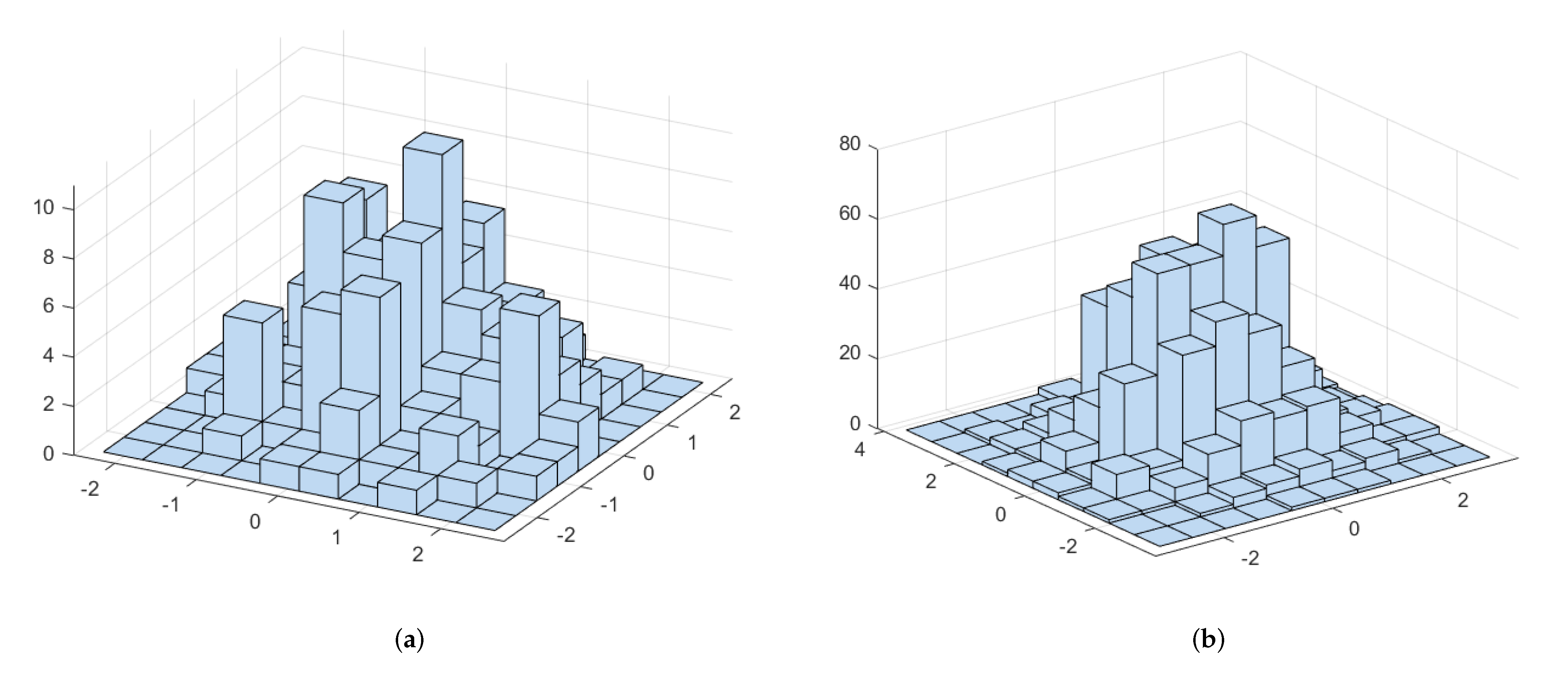
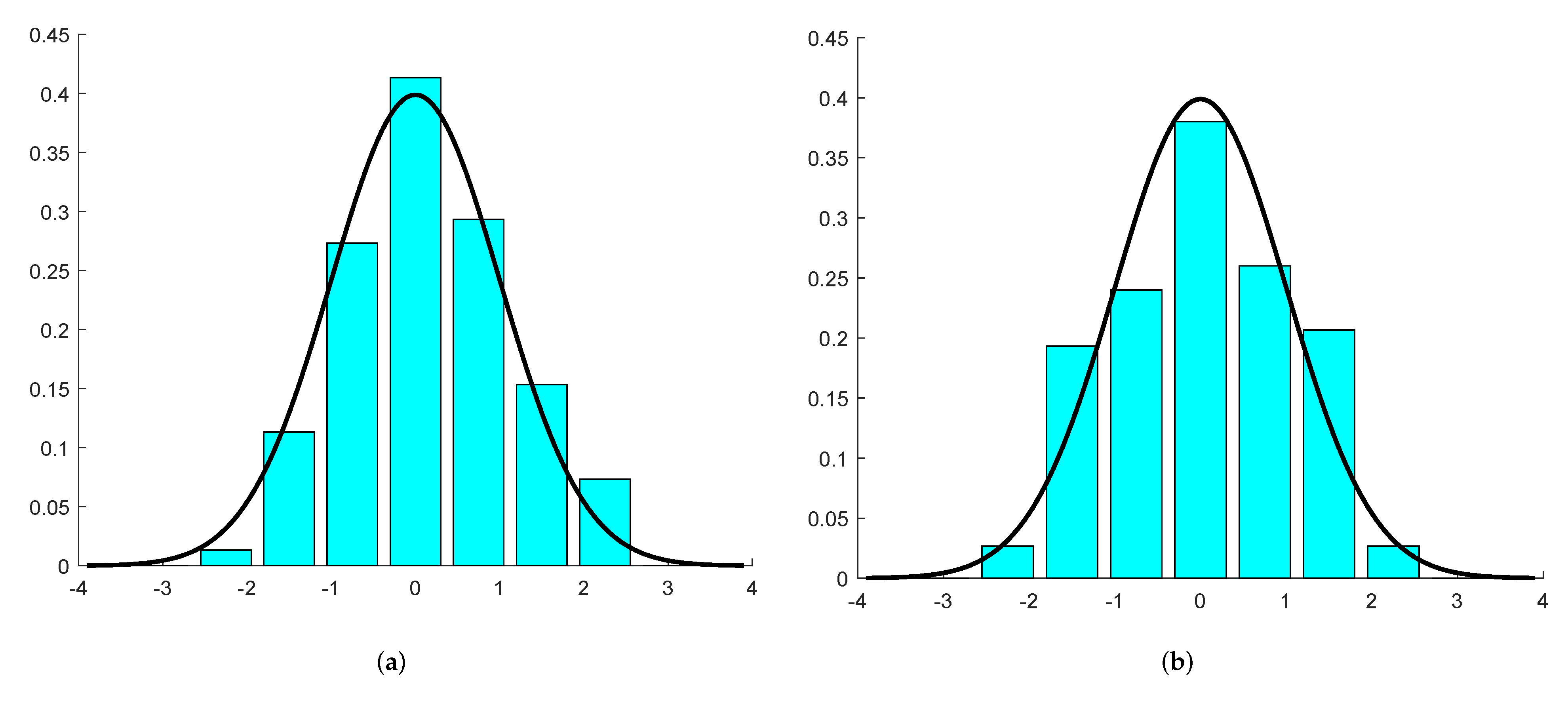
To this end, we propose the following ${\chi }^2$-test. Let

$${\chi }_o^2=\sum _{j=1}^m\frac{{\left(n_j-2n\frac{\left[t_{j}N\right]-\left[t_{j-1}N\right]}{N}\right)}^2}{2n(t_j-t_{j-1})}$$

be the test statistic.

Let $0<\alpha <1$. Choose the critical value ${\chi }_c^2$, such that $\mathbb{P}\{{\chi }^2(m-1)<{\chi }_c^2\}=1-\alpha$, where ${\chi }^2(m-1)$ is a random variable having ${\chi }^2$-distribution with a degree of freedom of $m-1$. The hypothesis $H_0$ is accepted if ${\chi }_o^2<{\chi }_c^2$, and it is rejected if ${\chi }_o^2\ge {\chi }_c^2$. By Theorem 4, if $\frac{n}{N}\to \infty$, then the probability of the type I error converges to

$$\mathbb{P}\{{\chi }^2(m-1)\ge {\chi }_c^2\}=\alpha .$$

Above we used, besides Theorem 4, the following known fact from the statistical theory of ${\chi }^2$-tests. If $t_0=0<t_1<\dots <t_m=1$, then, for the increments of the Brownian bridge $W_0$, the distribution of

$$\sum _{j=1}^m\frac{{\left(W_0\left(t_j\right)-W_0(t_{j-1}\right)}^2}{t_j-t_{j-1}}$$

is ${\chi }^2(m-1)$.

Example 3.

We carried out computer experiments to show numerically the results of our theorems. We simulated the allocations using random numbers. We considered a homogeneous allocation, that is, when we allocate a particle, then we choose a cell uniformly at random from the N cells. We allocated $2n=1000$ particles into $N=20$ cells. We repeated this experiment several times and we only saved those results when there was an even number of particles in each cell. So we saved $s=200$ times the results of the allocations. In this way, we obtained a sample of size $s=200$ for our $N=20$-dimensional random vector ${\eta }_1^{\prime },\dots ,{\eta }_N^{\prime }$. Then, we constructed histograms for the fist two coordinates of the above-mentioned $N=20$-dimensional sample. On the left-hand side of Figure 1, the histogram of the observations of $\frac{{\eta }_1^{\prime }-2n{q}_1}{\sqrt{2n{q}_1}}$, together with the standard normal probability density function, are shown. On the right-hand side of Figure 1, the histogram for $\frac{{\eta }_2^{\prime }-2n{q}_2}{\sqrt{2n{q}_2}}$ and the standard normal probability density function can be seen. The fit to the normal distribution seems to be very good. On the left-hand side of Figure 2, the joint histogram of the sample for the variables $\frac{{\eta }_1^{\prime }-2n{q}_1}{\sqrt{2n{q}_1}}$ and $\frac{{\eta }_2^{\prime }-2n{q}_2}{\sqrt{2n{q}_2}}$ is given. This figure supports the joint normality of the two coordinates.Therefore, we obtained numerical evidence for Theorems 2 and 3. Finally, we performed principal component analysis for the observations of the vector

$$\frac{{\eta }_1^{\prime }-2n{q}_1}{\sqrt{2n{q}_1}},\dots ,\frac{{\eta }_N^{\prime }-2n{q}_N}{\sqrt{2n{q}_N}}.$$

Figure 1. The histograms of the first and the second coordinates in Example 3. (a) First coordinate; (b) Second coordinate.

The first 19 principal component variances were between $1.64$ and $0.53$, but the last one was zero; this result supports the theory that the degree of freedom of the ${\chi }^2$-statistic in Example 2 is $m-1$.

Example 4.

We carried out the same computer experiment as in Example 3, but using other parameters. We allocated $2n=2000$ particles into $N=10$ cells. We saved $s=1000$ times the results of those allocations when there was an even number of particles in each cell. In this way, we obtained a sample of size $s=1000$ for the $N=10$-dimensional random vector ${\eta }_1^{\prime },\dots ,{\eta }_N^{\prime }$. On the left-hand side of Figure 3, the histogram of the observations of $\frac{{\eta }_1^{\prime }-2n{q}_1}{\sqrt{2n{q}_1}}$, together with the standard normal probability density function, are presented. On the right-hand side of Figure 3, the histogram for $\frac{{\eta }_2^{\prime }-2n{q}_2}{\sqrt{2n{q}_2}}$ and the standard normal probability density function are given. The fit to the normal distribution is again, very good. On the right-hand side of Figure 2, the joint histogram of the sample for the variables $\frac{{\eta }_1^{\prime }-2n{q}_1}{\sqrt{2n{q}_1}}$ and $\frac{{\eta }_2^{\prime }-2n{q}_2}{\sqrt{2n{q}_2}}$ is given. This figure also supports the joint normality of the two coordinates. Therefore, we obtained another numerical confirmation for Theorems 2 and 3. Then, we performed principal component analysis for the observations of the vector

$$\frac{{\eta }_1^{\prime }-2n{q}_1}{\sqrt{2n{q}_1}},\dots ,\frac{{\eta }_N^{\prime }-2n{q}_N}{\sqrt{2n{q}_N}}.$$

The first 9 principal component variances were between $1.17$ and $0.87$, but the last one was zero. It supports that the degree of freedom of the ${\chi }^2$-statistic in Example 2 is $m-1$ and not m.

We mention that for relatively small values of n, e.g., for $2n=500$ and $N=25$, the numerical results show a pure fit to the normal distribution. It is also worth mentioning that we need a large sample size, i.e., $s>100$, to numerically show the goodness of fit to the normal distribution.

Figure 2. The joint histograms of the first two coordinates in Examples 3 and 4. (a) Histogram for Example 3; (b) Histogram for Example 4.

Figure 3. The histograms of the first and the second coordinates in Example 4. (a) First coordinate; (b) Second coordinate.

4. Auxiliary Results

We shall use the following notation. Let $\pi \left(\beta \right)$ denote a Poisson random variable with the parameter $\beta$, and let ${\xi }^{\prime }\left(\beta \right)$, where $\beta >0$, be a random variable with the distribution

$$\mathbb{P}\{{\xi }^{\prime }\left(\beta \right)=2k\}=\frac{{\beta }^{2k}}{\left(2k\right)!\mathrm{ch}\left(\beta \right)},k=0,1,2\dots .$$

Recall that this distribution appears in Theorem 1. We see that the distribution of ${\xi }^{*}\left(\beta \right)$ is the same as the distribution of ${\xi }^{\prime }\left(\beta \right)/2$.

Lemma 1.

Let $C>0$ be fixed. Then, we have

$$\mathbb{P}\{{\xi }^{\prime }\left(\beta \right)=2k\}=\frac{2}{\sqrt{2\pi \beta }}\left(exp\left(-\frac{{(2k-\beta )}^2}{2\beta }\right)\right)(1+\mathrm{o}\left(1\right))$$

(18)

as $\beta \to \infty$, uniformly for those values of k for which $\frac{|2k-\beta |}{\sqrt{\beta }}<C$.

Proof. 

We need the following approximation of the Poisson distribution by the normal density function, see p. 43 of [7]. Let $\tau$ have Poisson distribution $\mathbb{P}(\tau =k)=\frac{{\lambda }^k}{k!}{e}^{-\lambda }$, $k=0,1,2,\dots$ and let $k=\lambda +x\sqrt{\lambda }$. Then, as $\lambda \to \infty$,

$$\mathbb{P}(\tau =k)=\frac{1}{\sqrt{2\pi \lambda }}{e}^{-\frac{x^2}{2}}\left(1+\mathrm{O}\left(\frac{1}{\sqrt{\lambda }}\right)\right),$$

uniformly for $x\in [-c,c]$, where c is an arbitrary fixed positive number.

Using the above approximation for $\mathbb{P}\left\{\pi \right(\beta )=2k\}$, we obtain

$$\mathbb{P}\{{\xi }^{\prime }\left(\beta \right)=2k\}=\frac{{\beta }^{2k}}{\left(2k\right)!e^{\beta }}\frac{1}{\frac{1}{2}(1+e^{-2\beta })}=\mathbb{P}\{\pi \left(\beta \right)=2k\}\frac{1+\mathrm{o}\left(1\right)}{\frac{1}{2}}$$

$$=\frac{1}{\sqrt{2\pi \beta }}\left(exp\left(-\frac{{(2k-\beta )}^2}{2\beta }\right)\right)(1+\mathrm{o}\left(1\right))\frac{1+\mathrm{o}\left(1\right)}{\frac{1}{2}}$$

$$=\frac{2}{\sqrt{2\pi \beta }}\left(exp\left(-\frac{{(2k-\beta )}^2}{2\beta }\right)\right)(1+\mathrm{o}\left(1\right))$$

as $\beta \to \infty$ uniformly for k such that $\frac{|2k-\beta |}{\sqrt{\beta }}<C$. □

Lemma 2.

For the moments of ${\xi }^{*}\left(\beta \right)$, we have

$$\begin{array}{cc}\hfill & m^{*}\left(\beta \right)=\mathbb{E}{\xi }^{*}\left(\beta \right)=\frac{\beta }{2}\mathrm{th}\left(\beta \right),{\sigma }^{*2}\left(\beta \right)={\mathbb{D}}^2{\xi }^{*}\left(\beta \right)=\frac{\beta }{4}\left(1+\mathrm{o}\left(1\right)\right),\hfill \\ \hfill & \mathbb{E}{({\xi }^{*}\left(\beta \right)-\mathbb{E}{\xi }^{*}\left(\beta \right))}^4=\frac{3}{16}{\beta }^2(1+\mathrm{o}\left(1\right))\hfill \end{array}$$

(19)

as $\beta \to \infty$.

Proof. 

By simple calculation, one can obtain that the characteristic function of ${\xi }^{*}\left(\beta \right)$ is

$$\varphi \left(t\right)=\frac{\mathrm{ch}\left(\beta e^{\frac{it}{2}}\right)}{\mathrm{ch}\left(\beta \right)},t\in \mathbb{R},$$

(20)

where $i=\sqrt{-1}$. Using the hyperbolic sine function $\mathrm{sh}\left(x\right)=\frac{e^x-e^{-x}}{2}$, we can obtain the derivatives of the characteristic function

$${\varphi }^{\prime }\left(t\right)=\frac{\mathrm{sh}\left(\beta e^{\frac{it}{2}}\right)}{\mathrm{ch}\left(\beta \right)}\beta e^{\frac{it}{2}}\frac{i}{2},$$

$${\varphi }^{″}\left(t\right)=\frac{\mathrm{ch}\left(\beta e^{\frac{it}{2}}\right)}{\mathrm{ch}\left(\beta \right)}{\left(\beta e^{\frac{it}{2}}\frac{i}{2}\right)}^2+\frac{\mathrm{sh}\left(\beta e^{\frac{it}{2}}\right)}{\mathrm{ch}\left(\beta \right)}\beta e^{\frac{it}{2}}\frac{(-1)}{4},$$

$${\varphi }^{‴}\left(t\right)=\frac{\mathrm{sh}\left(\beta e^{\frac{it}{2}}\right)}{\mathrm{ch}\left(\beta \right)}{\left(\beta e^{\frac{it}{2}}\frac{i}{2}\right)}^3+\frac{\mathrm{ch}\left(\beta e^{\frac{it}{2}}\right)}{\mathrm{ch}\left(\beta \right)}{\beta }^2{e}^{it}\frac{(-i)}{4}+\frac{\mathrm{ch}\left(\beta e^{\frac{it}{2}}\right)}{\mathrm{ch}\left(\beta \right)}{\beta }^2{e}^{it}\frac{(-i)}{8}+\frac{\mathrm{sh}\left(\beta e^{\frac{it}{2}}\right)}{\mathrm{ch}\left(\beta \right)}\beta e^{\frac{it}{2}}\frac{(-i)}{8}$$

$$=\frac{\mathrm{sh}\left(\beta e^{\frac{it}{2}}\right)}{\mathrm{ch}\left(\beta \right)}{\left(\beta e^{\frac{it}{2}}\frac{i}{2}\right)}^3+3\frac{\mathrm{ch}\left(\beta e^{\frac{it}{2}}\right)}{\mathrm{ch}\left(\beta \right)}{\beta }^2{e}^{it}\frac{(-i)}{8}+\frac{\mathrm{sh}\left(\beta e^{\frac{it}{2}}\right)}{\mathrm{ch}\left(\beta \right)}\beta e^{\frac{it}{2}}\frac{(-i)}{8},$$

and

$${\varphi }^{iv}\left(t\right)=\frac{\mathrm{ch}\left(\beta e^{\frac{it}{2}}\right)}{\mathrm{ch}\left(\beta \right)}{\left(\beta e^{\frac{it}{2}}\frac{i}{2}\right)}^4+3\frac{\mathrm{sh}\left(\beta e^{\frac{it}{2}}\right)}{\mathrm{ch}\left(\beta \right)}{\beta }^3{e}^{i\frac{3t}{2}}\frac{1}{16}+\frac{\mathrm{ch}\left(\beta e^{\frac{it}{2}}\right)}{\mathrm{ch}\left(\beta \right)}{\beta }^2{e}^{it}\frac{1}{16}$$

$$+3\frac{\mathrm{sh}\left(\beta e^{\frac{it}{2}}\right)}{\mathrm{ch}\left(\beta \right)}{\left(\beta e^{\frac{it}{2}}\frac{i}{2}\right)}^2\beta e^{\frac{it}{2}}\frac{(-1)}{4}+3\frac{\mathrm{ch}\left(\beta e^{\frac{it}{2}}\right)}{\mathrm{ch}\left(\beta \right)}{\beta }^2{e}^{it}\frac{1}{8}+\frac{\mathrm{sh}\left(\beta e^{\frac{it}{2}}\right)}{\mathrm{ch}\left(\beta \right)}\beta e^{\frac{it}{2}}\frac{1}{16}$$

$$=\frac{\mathrm{ch}\left(\beta e^{\frac{it}{2}}\right)}{\mathrm{ch}\left(\beta \right)}{\left(\beta e^{\frac{it}{2}}\frac{i}{2}\right)}^4+6\frac{\mathrm{sh}\left(\beta e^{\frac{it}{2}}\right)}{\mathrm{ch}\left(\beta \right)}{\beta }^3{e}^{i\frac{3t}{2}}\frac{1}{16}+7\frac{\mathrm{ch}\left(\beta e^{\frac{it}{2}}\right)}{\mathrm{ch}\left(\beta \right)}{\beta }^2{e}^{it}\frac{1}{16}+\frac{\mathrm{sh}\left(\beta e^{\frac{it}{2}}\right)}{\mathrm{ch}\left(\beta \right)}\beta e^{\frac{it}{2}}\frac{1}{16}.$$

Therefore, we obtain

$$m^{*}\left(\beta \right)=\mathbb{E}{\xi }^{*}\left(\beta \right)=-i{\varphi }^{\prime }\left(0\right)=\frac{\beta }{2}\mathrm{th}\left(\beta \right).$$

(21)

Moreover,

$$\mathbb{E}{\left({\xi }^{*}\left(\beta \right)\right)}^2=-{\varphi }^{″}\left(0\right)=\frac{{\beta }^2}{4}+\frac{\beta }{4}\mathrm{th}\left(\beta \right),$$

(22)

$$\mathbb{E}{\left({\xi }^{*}\left(\beta \right)\right)}^3=i{\varphi }^{‴}\left(0\right)=\frac{{\beta }^3}{8}\mathrm{th}\left(\beta \right)+\frac{3}{8}{\beta }^2+\frac{\beta }{8}\mathrm{th}\left(\beta \right),$$

(23)

and

$$\mathbb{E}{\left({\xi }^{*}\left(\beta \right)\right)}^4={\varphi }^{iv}\left(0\right)=\frac{1}{16}{\beta }^4+\frac{6{\beta }^3}{16}\mathrm{th}\left(\beta \right)+\frac{7}{16}{\beta }^2+\frac{\beta }{16}\mathrm{th}\left(\beta \right).$$

(24)

From Equations (21)–(24), it follows that

$${\sigma }^{*2}\left(\beta \right)={\mathbb{D}}^2\left({\xi }^{*}\left(\beta \right)\right)=\mathbb{E}{\left({\xi }^{*}\left(\beta \right)\right)}^2-{\left(\mathbb{E}{\xi }^{*}\left(\beta \right)\right)}^2$$

$$=\frac{{\beta }^2}{4}+\frac{\beta }{4}\mathrm{th}\left(\beta \right)-{\left(\frac{\beta }{2}\mathrm{th}\left(\beta \right)\right)}^2=\frac{{\beta }^2}{4{\mathrm{ch}}^2\left(\beta \right)}+\frac{\beta }{4}\mathrm{th}\left(\beta \right)=\frac{\beta }{4}\left(1+\frac{\beta }{{\mathrm{ch}}^2\left(\beta \right)}-\frac{e^{-\beta }}{\mathrm{ch}\left(\beta \right)}\right).$$

(25)

It implies that ${\sigma }^{*2}\left(\beta \right)=\frac{\beta }{4}\left(1+\mathrm{o}\left(1\right)\right)$. Then

$$\mathbb{E}{({\xi }^{*}\left(\beta \right)-\mathbb{E}{\xi }^{*}\left(\beta \right))}^4$$

$$=\mathbb{E}{\left({\xi }^{*}\left(\beta \right)\right)}^4-4\left(\mathbb{E}{\left({\xi }^{*}\left(\beta \right)\right)}^3\right)\mathbb{E}{\xi }^{*}\left(\beta \right)+6\left(\mathbb{E}{\left({\xi }^{*}\left(\beta \right)\right)}^2\right){\left(\mathbb{E}{\xi }^{*}\left(\beta \right)\right)}^2-3{\left(\mathbb{E}{\xi }^{*}\left(\beta \right)\right)}^4$$

$$=\frac{1}{16}{\beta }^4+\frac{6{\beta }^3}{16}\mathrm{th}\left(\beta \right)+\frac{7}{16}{\beta }^2+\frac{\beta }{16}\mathrm{th}\left(\beta \right)-4\left(\frac{{\beta }^3}{8}\mathrm{th}\left(\beta \right)+\frac{3}{8}{\beta }^2+\frac{\beta }{8}\mathrm{th}\left(\beta \right)\right)\frac{\beta }{2}\mathrm{th}\left(\beta \right)$$

$$+6\left(\frac{{\beta }^2}{4}+\frac{\beta }{4}\mathrm{th}\left(\beta \right)\right){\left(\frac{\beta }{2}\mathrm{th}\left(\beta \right)\right)}^2-3{\left(\frac{\beta }{2}\mathrm{th}\left(\beta \right)\right)}^4$$

$$=\frac{2{\beta }^4}{16}\left({\mathrm{th}}^2\left(\beta \right)-1\right)-\frac{3{\beta }^4}{16}\left({\mathrm{th}}^4\left(\beta \right)-1\right)-\frac{6{\beta }^3}{16}\left(\mathrm{th}\left(\beta \right)-1\right)+\frac{6{\beta }^3}{16}\left({\mathrm{th}}^3\left(\beta \right)-1\right)$$

$$+\frac{3}{16}{\beta }^2-\frac{4{\beta }^2}{16}\left({\mathrm{th}}^2\left(\beta \right)-1\right)+\frac{\beta }{16}+\frac{\beta }{16}\left(\mathrm{th}\left(\beta \right)-1\right).$$

(26)

Since

$${\beta }^k({\mathrm{th}}^l\left(\beta \right)-1)\to 0\mathrm{and}\mathrm{th}\left(\beta \right)\to 1\mathrm{as}\beta \to \infty ,$$

for $k,l=1,2,3,4$, we obtain

$$\mathbb{E}{({\xi }^{*}\left(\beta \right)-\mathbb{E}{\xi }^{*}\left(\beta \right))}^4=\frac{3}{16}{\beta }^2+\frac{1}{16}\beta +\mathrm{o}\left(1\right)=\frac{3}{16}{\beta }^2(1+\mathrm{o}\left(1\right)).$$

Thus, (19) is proved. □

We shall use the following general Berry–Esseen-type inequality. We should mention that in the following Lemma 3, there is no assumption on the distributions of the random variables ${\xi }_i$, $1\le i\le N$.

Lemma 3.

Let ${\xi }_i$, $1\le i\le N$, be independent random variables with variances ${\sigma }_i^2$ and expectations $m_i$, $i=1,2,\dots ,N$. Let $S_N={\sum }_{i=1}^N{\xi }_i$, and let $d_N^2={\sum }_{i=1}^N{\sigma }_i^2$ be its variance and let ${\mu }_N={\sum }_{i=1}^N{m}_i$ be its expectation. Then, we have

$$\underset{t\in \mathbb{R}}{sup}\left|\mathbb{P}\left\{\frac{S_N-{\mu }_N}{d_N}<t\right\}-\Phi \left(t\right)\right|\le 2c{\left(\frac{{\sum }_{i=1}^N\mathbb{E}{({\xi }_i-m_i)}^4}{d_N^4}\right)}^{\frac{1}{2}}.$$

(27)

Here, Φ is the standard normal distribution function and c is the constant from the Berry–Esseen inequality.

Lemma 3 was proved in [2]. Now, we shall apply Lemma 3 to our model.

Lemma 4.

Assume that for the random variables

$${\xi }_1^{*},{\xi }_2^{*},\dots ,{\xi }_N^{*}$$

from formula (9), condition (12) is valid. Then, for their standardized sum, we have

$$\frac{S_N^{*}-m_N^{*}}{{\sigma }_N^{*}}\stackrel{d}{\to }\gamma .$$

Proof. 

Using (19) for the right-hand side of (27), we obtain

$$\underset{t\in \mathbb{R}}{sup}\left|\mathbb{P}\left\{\frac{S_N^{*}-m_N^{*}}{{\sigma }_N^{*}}<t\right\}-\Phi \left(t\right)\right|\le 2c{\left(\frac{3\left({\sum }_{i=1}^N{\left({\beta }_i\right)}^2\right)(1+\mathrm{o}\left(1\right))}{{\left({\sum }_{i=1}^N{\beta }_i\right)}^2}\right)}^{\frac{1}{2}}$$

$$\le 2c{\left(\frac{3\left({max}_{1\le i\le N}{\beta }_i\right)(1+\mathrm{o}\left(1\right))}{{\sum }_{i=1}^N{\beta }_i}\right)}^{\frac{1}{2}}.$$

(28)

Now, (28) implies Lemma 4. □

In the following lemma, we shall need the characteristic functions of the random variables in (9). Thus, let

$${\varphi }_j\left(t\right)=\frac{\mathrm{ch}\left({\beta }_j{e}^{i\frac{t}{2}}\right)}{\mathrm{ch}\left({\beta }_j\right)}=\frac{e^{{\beta }_j{e}^{i\frac{t}{2}}}+e^{-{\beta }_j{e}^{i\frac{t}{2}}}}{e^{{\beta }_j}+e^{-{\beta }_j}}$$

be the characteristic function of ${\xi }_j^{*}$, let ${\varphi }_j^c\left(t\right)={\varphi }_j\left(t\right)e^{-it{m}^{*}\left({\beta }_j\right)}$ be the characteristic function of the centralized version of ${\xi }_j^{*}$, $1\le j\le N$, and let ${\varphi }_N\left(t\right)$ be the characteristic function of the standardized sum $\frac{S_N^{*}-m_N^{*}}{{\sigma }_N^{*}}$.

Lemma 5.

Assume that for the random variables

$${\xi }_1^{*},{\xi }_2^{*},\dots ,{\xi }_N^{*}$$

from formula (9), condition (12) is valid. Let $C>0$. Then, we have

$${\sigma }_N^{*}\mathbb{P}\{S_N^{*}=n\}=\frac{1}{\sqrt{2\pi }}exp\left(-\frac{{(n-m_N^{*})}^2}{2{\sigma }_N^{*2}}\right)(1+\mathrm{o}\left(1\right)),$$

(29)

uniformly for those n, such that $\frac{|n-m_N^{*}|}{{\sigma }_N^{*}}<C$.

Proof. 

We shall need the notation

$$z=\frac{n-m_N^{*}}{{\sigma }_N^{*}}.$$

$S_N^{*}$ is an integer valued random variable, so its distribution can be expressed by the following inverse Fourier transform

$$\mathbb{P}\{S_N^{*}=n\}=\frac{1}{2\pi }{\int }_{-\pi }^{\pi }{e}^{-inx}{\varphi }_N^0\left(x\right)dx,$$

(30)

where ${\varphi }_N^0$ is the characteristic function of $S_N^{*}$. However,

$${\varphi }_N^0\left(\frac{t}{{\sigma }_N^{*}}\right)={\varphi }_N\left(t\right)e^{\frac{it{m}_N^{*}}{{\sigma }_N^{*}}}=\prod _{j=1}^N{\varphi }_j^c\left(\frac{t}{{\sigma }_N^{*}}\right)e^{\frac{it{m}_N^{*}}{{\sigma }_N^{*}}}.$$

So, substituting $x=t/{\sigma }_N^{*}$ into the integral in (30), we obtain

$${\sigma }_N^{*}\mathbb{P}\{S_N^{*}=n\}=\frac{1}{2\pi }{\int }_{-\pi {\sigma }_N^{*}}^{\pi {\sigma }_N^{*}}{e}^{-itz}{\varphi }_N\left(t\right)dt=\frac{1}{2\pi }{\int }_{-\pi {\sigma }_N^{*}}^{\pi {\sigma }_N^{*}}{e}^{-itz}\prod _{i=1}^N{\varphi }_i^c\left(\frac{t}{{\sigma }_N^{*}}\right)dt.$$

Let $0<\epsilon <1$ and $B>0$. Using the characteristic function of the standard normal law, we have, for any real z, that

$$\frac{1}{\sqrt{2\pi }}{e}^{-\frac{z^2}{2}}=\frac{1}{2\pi }{\int }_{-\infty }^{\infty }{e}^{-ixz}{e}^{-\frac{x^2}{2}}dx.$$

So we can represent the difference of the two sides of (29) as the sum of four integrals

$$R_N=2\pi \left({\sigma }_N^{*}\mathbb{P}\{S_N^{*}=n\}-\frac{1}{\sqrt{2\pi }}{e}^{-\frac{z^2}{2}}\right)=I_1+I_2+I_3+I_4,$$

(31)

where

$$I_1={\int }_{\left|x\right|<B}{e}^{-ixz}{\varphi }_N\left(x\right)dx-{\int }_{\left|x\right|<B}{e}^{-ixz}{e}^{-\frac{x^2}{2}}dx,$$

$$I_2=-{\int }_{\left|x\right|>B}{e}^{-ixz}{e}^{-\frac{x^2}{2}}dx,$$

$$I_3={\int }_{B<\left|x\right|\le \epsilon {\sigma }_N^{*}}{e}^{-ixz}\left(\prod _{j=1}^N{\varphi }_j^c\left(\frac{x}{{\sigma }_N^{*}}\right)\right)dx$$

and

$$I_4={\int }_{\epsilon {\sigma }_N^{*}<\left|x\right|\le \pi {\sigma }_N^{*}}{e}^{-ixz}\left(\prod _{j=1}^N{\varphi }_j^c\left(\frac{x}{{\sigma }_N^{*}}\right)\right)dx.$$

Since

$$I_1={\int }_{\left|x\right|<B}{e}^{-ixz}\left({\varphi }_N\left(x\right)-e^{-\frac{x^2}{2}}\right)dx,$$

from Lemma 4, it follows that

$$I_1\to 0$$

(32)

for all fixed $B>0$.

Since

$$|I_2|<{\int }_{\left|x\right|>B}{e}^{-\frac{x^2}{2}}dx,$$

we have

$$I_2\to 0\mathrm{as}B\to \infty .$$

(33)

Using formula (20) for the characteristic function of ${\xi }^{*}\left(\beta \right)$, we obtain

$$|I_3|\le {\int }_{B<\left|x\right|\le \epsilon {\sigma }_N^{*}}\left|e^{-ixz}\left(\prod _{j=1}^N{\varphi }_j^c\left(\frac{x}{{\sigma }_N^{*}}\right)\right)\right|dx$$

$$={\int }_{B<\left|t\right|\le \epsilon {\sigma }_N^{*}}\left(\prod _{j=1}^N{e}^{{\beta }_j\left(cos\frac{t}{2{\sigma }_N^{*}}-1\right)}\right)\prod _{j=1}^N\left|\frac{1+e^{-2{\beta }_j{e}^{i\frac{t}{2{\sigma }_N^{*}}}}}{1+e^{-2{\beta }_j}}\right|dt.$$

We know that

$$cos\left(x\right)-1\le -\frac{x^2}{2}+\frac{x^4}{24}\le -\frac{11x^2}{24},\mathrm{if}\left|x\right|\le 1;e^x-1\le x{e}^x,\mathrm{if}x\ge 0.$$

Therefore, we obtain that

$$\prod _{j=1}^N{e}^{{\beta }_j\left(cos\frac{t}{2{\sigma }_N^{*}}-1\right)}\le e^{-\left({\sum }_{j=1}^N{\beta }_j\right)\frac{11·t^2}{24·4{\sigma }_N^{*2}}}\le e^{-\frac{11t^2}{24·4(1+\mathrm{o}(1\left)\right)}}$$

as $B<\left|t\right|\le \epsilon {\sigma }_N^{*}$, where we applied that ${\sigma }^{*2}\left({\beta }_j\right)=\frac{{\beta }_j}{4}(1+\mathrm{o}\left(1\right))$. Moreover,

$$\prod _{j=1}^N\left|\frac{1+e^{-2{\beta }_j{e}^{i\frac{t}{2{\sigma }_N^{*}}}}}{1+e^{-2{\beta }_j}}\right|\le \prod _{j=1}^N\frac{1+e^{-2{\beta }_{j}cos\left(\frac{t}{2{\sigma }_N^{*}}\right)}}{1+e^{-2{\beta }_j}}$$

$$=\prod _{j=1}^N\left(1+\frac{e^{-2{\beta }_{j}cos\left(\frac{t}{2{\sigma }_N^{*}}\right)}-e^{-2{\beta }_j}}{1+e^{-2{\beta }_j}}\right)=exp\left(\sum _{j=1}^{N}ln\left(1+\frac{e^{-2{\beta }_{j}cos\left(\frac{t}{2{\sigma }_N^{*}}\right)}-e^{-2{\beta }_j}}{1+e^{-2{\beta }_j}}\right)\right)$$

$$\le exp\left(\sum _{j=1}^N{e}^{-2{\beta }_j}\frac{e^{2{\beta }_j\left(1-cos\left(\frac{t}{2{\sigma }_N^{*}}\right)\right)}-1}{1+e^{-2{\beta }_j}}\right)\le exp\left(\sum _{j=1}^N{e}^{-2{\beta }_j}\frac{2{\beta }_j\left(1-cos\left(\frac{t}{2{\sigma }_N^{*}}\right)\right)}{1+e^{-2{\beta }_j}}\right)$$

$$\le exp\left(\sum _{j=1}^N{e}^{-2{\beta }_j}\frac{2{\beta }_j\frac{11}{24}{\left(\frac{t}{2{\sigma }_N^{*}}\right)}^2}{1+e^{-2{\beta }_j}}\right)\le exp\left(\frac{11}{12}·\frac{exp(-2{min}_{1\le j\le N}{\beta }_j)t^2}{(1+\mathrm{o}(1\left)\right)}\right)=e^{t^2\mathrm{o}\left(1\right)},$$

$B<\left|t\right|\le \epsilon {\sigma }_N^{*}$. Here, we used that $e^x\ge x+1$, the shape of ${\sigma }_N^{*}$ and condition (12). Therefore, we obtain

$$|I_3|\le {\int }_{B<\left|t\right|\le \epsilon {\sigma }_N^{*}}\left(e^{-\frac{10t^2}{24}(1+\mathrm{o}\left(1\right))}\right)dt\le {\int }_{B<\left|t\right|}\left(e^{-\frac{10t^2}{24}(1+\mathrm{o}\left(1\right))}\right)dt.$$

Consequently,

$$|I_3|\to 0\mathrm{as}B\to \infty .$$

(34)

Now, we turn to $I_4$. By (20), we have

$$|{\varphi }_j\left(x\right)|=\left|\frac{e^{{\beta }_j{e}^{i\frac{x}{2}}}+e^{-{\beta }_j{e}^{i\frac{x}{2}}}}{e^{{\beta }_j}+e^{-{\beta }_j}}\right|$$

$$\le \frac{e^{{\beta }_{j}cos\left(\frac{x}{2}\right)}+e^{-{\beta }_{j}cos\left(\frac{x}{2}\right)}}{e^{{\beta }_j}+e^{-{\beta }_j}}\le \frac{e^{{\beta }_{j}cos\left(\epsilon \right)}+e^{-{\beta }_{j}cos\left(\epsilon \right)}}{e^{{\beta }_j}+e^{-{\beta }_j}}=\frac{\mathrm{ch}({\beta }_{j}cos\left(\epsilon \right))}{\mathrm{ch}\left({\beta }_j\right)}$$

for $\epsilon <\left|x\right|\le \pi$. Thus,

$$|I_4|\le 2\pi {\sigma }_N^{*}\prod _{j=1}^N\left(\frac{\mathrm{ch}({\beta }_{j}cos\left(\epsilon \right))}{\mathrm{ch}\left({\beta }_j\right)}\right)\le 2\pi {\sigma }_N^{*}\prod _{j=1}^N\left(e^{-(1-cos\left(\epsilon \right)){\beta }_j}\frac{1+e^{-2{\beta }_{j}cos\left(\epsilon \right)}}{1+e^{-2{\beta }_j}}\right).$$

Since, by (12), ${min}_{1\le j\le N}{\beta }_j\to \infty$; therefore, we have

$$\frac{1+e^{-2{\beta }_{j}cos\left(\epsilon \right)}}{1+e^{-2{\beta }_j}}\to 1$$

as $N\to \infty$, uniformly for $1\le i\le N$. Consequently, there exists $N_0\in \mathbb{N}$, such that

$$\frac{1+e^{-2{\beta }_{j}cos\left(\epsilon \right)}}{1+e^{-2{\beta }_j}}<e^{\frac{1}{2}(1-cos\left(\epsilon \right)){\beta }_j},$$

$1\le j\le N$, $N>N_0$. Therefore,

$$|I_4|\le 2\pi {\sigma }_N^{*}\prod _{j=1}^N{e}^{-\frac{1}{2}(1-cos\left(\epsilon \right)){\beta }_j}\le 2\pi {\sigma }_N^{*}{e}^{-\frac{1}{2}(1-cos\left(\epsilon \right)){\sigma }_N^{*2}(1+\mathrm{o}\left(1\right))}$$

for $N>N_0$. Therefore, we obtain that

$$I_4\to 0.$$

(35)

Finally, using formulae (32), (33), (34), and (35) to approximate the left-hand side of (31), we obtain (29). □

5. Proofs of the Main Theorems

Proof of Theorem 2.

During the proof, we represent ${\eta }_1^{\prime },{\eta }_2^{\prime },\dots ,{\eta }_N^{\prime }$ in the form of (7). First, we prove a local version of our limit theorem. To this end, we study the case when the standardized random variables are inside some bounded intervals. Therefore, we need the following notation. Let $C_{1i}<C_{2i}$, $1\le i\le K$. Let

$$k=\sum _{i=1}^K{k}_i,C^{*}=max\left\{\right|C_{ij}|:1\le j\le K,i=1,2,\}.$$

Let

$$m_K^{*}=\sum _{i=K+1}^N{m}^{*}\left({\beta }_i\right)\mathrm{and}{\sigma }_K^{*2}=\sum _{i=K+1}^N{\sigma }^{*2}\left({\beta }_i\right)$$

be the expectation and the variance of ${\sum }_{i=K+1}^N{\xi }_i^{*}$. By Lemma 1, we have

$$\prod _{i=1}^K\mathbb{P}({\xi }_i^{\prime }=2k_i)=\prod _{i=1}^K\frac{2}{\sqrt{2\pi {\beta }_i}}\left(exp\left(-\frac{{(2k_i-{\beta }_i)}^2}{2{\beta }_i}\right)\right)(1+\mathrm{o}\left(1\right)),$$

(36)

uniformly for $k_i$, $1\le i\le K$, such that

$$C_{1i}<\frac{2k_i-{\beta }_i}{\sqrt{{\beta }_i}}<C_{2i},1\le i\le K.$$

(37)

Since

$${\sigma }_N^{*2}\ge {\sigma }_K^{*2}=\sum _{i=K+1}^N\frac{{\beta }_i}{4}\left(1+\frac{{\beta }_i}{{\mathrm{ch}}^2\left({\beta }_i\right)}-\frac{e^{-{\beta }_i}}{\mathrm{ch}{\beta }_i}\right)$$

$$=\frac{1+\mathrm{o}\left(1\right)}{4}\sum _{i=K+1}^N{\beta }_i=\frac{1+\mathrm{o}\left(1\right)}{4}\left(\sum _{i=1}^N{\beta }_i\right)\left(1-\frac{{\sum }_{i=1}^K{\beta }_i}{{\sum }_{i=1}^N{\beta }_i}\right)$$

$$\ge \frac{1+\mathrm{o}\left(1\right)}{4}\left(\sum _{i=1}^N{\beta }_i\right)\left(1-\frac{K{max}_{1\le i\le K}{\beta }_i}{{\sum }_{i=1}^N{\beta }_i}\right)=(1+\mathrm{o}\left(1\right)){\sigma }_N^{*2},$$

Therefore, we have

$${\sigma }_K^{*2}=(1+\mathrm{o}\left(1\right)){\sigma }_N^{*2}\mathrm{and}\frac{{\sigma }_K^{*}}{{\sigma }_N^{*}}=\mathrm{o}\left(1\right).$$

Let $k_i$, $1\le i\le K$, be such that $C_{1i}<\frac{2k_i-{\beta }_i}{\sqrt{{\beta }_i}}<C_{2i}$ for $1\le i\le K$. Using (12) and the above calculation, we have

$$\frac{|n-k-m_K^{*}|}{{\sigma }_K^{*}}\le \frac{|n-m_N^{*}|}{{\sigma }_K^{*}}+\sum _{i=1}^K\frac{|k_i-m^{*}\left({\beta }_i\right)|}{{\sigma }_K^{*}}<C+K{C}^{*}+\mathrm{o}\left(1\right).$$

(38)

Therefore, by Lemma 5, we obtain

$$\frac{\mathbb{P}\left\{{\sum }_{i=K+1}^N{\xi }_i^{*}=n-k\right\}}{\mathbb{P}\left\{{\sum }_{i=1}^N{\xi }_i^{*}=n\right\}}=\frac{\frac{1}{\sqrt{2\pi }{\sigma }_K^{*}}exp\left(-\frac{{(n-k-m_K^{*})}^2}{2{\sigma }_K^{*2}}\right)(1+\mathrm{o}\left(1\right))}{\frac{1}{\sqrt{2\pi }{\sigma }_N^{*}}exp\left(-\frac{{(n-m_N^{*})}^2}{2{\sigma }_N^{*2}}\right)(1+\mathrm{o}\left(1\right))}$$

$$=exp\left(\frac{{(n-m_N^{*})}^2}{2{\sigma }_N^{*2}}-\frac{{(n-k-m_K^{*})}^2}{2{\sigma }_N^{*2}}\right)(1+\mathrm{o}\left(1\right))$$

$$=exp\left(\frac{(k-(m_N^{*}-m_K^{*}))}{{\sigma }_N^{*}}\frac{(n-m_N^{*}+n-k-m_K^{*})}{2{\sigma }_N^{*}}\right)(1+\mathrm{o}\left(1\right)).$$

Using (38), (37), and assumption (12), we obtain

$$\left|\frac{(n-m_N^{*}+n-k-m_K^{*})}{{\sigma }_N^{*}}\frac{(k-(m_N^{*}-m_K^{*}))}{{\sigma }_N^{*}}\right|\le (2C+K{C}^{*}+\mathrm{o}\left(1\right))\sum _{i=1}^K\frac{{\sigma }^{*}\left({\beta }_i\right)}{{\sigma }_N^{*}}\frac{|k_i-m^{*}\left({\beta }_i\right)|}{{\sigma }^{*}\left({\beta }_i\right)}$$

$$\le (2C+K{C}^{*}+\mathrm{o}\left(1\right))(C^{*}+\mathrm{o}\left(1\right))\sum _{i=1}^K\frac{{\sigma }^{*}\left({\beta }_i\right)}{{\sigma }_N^{*}}=\mathrm{o}\left(1\right).$$

Using the above calculations, we have

$$\frac{\mathbb{P}\left\{{\sum }_{i=K+1}^N{\xi }_i^{*}=n-k\right\}}{\mathbb{P}\left\{{\sum }_{i=1}^N{\xi }_i^{*}=n\right\}}=1+\mathrm{o}\left(1\right).$$

(39)

Now, using (36) and (39) in formula (7), we obtain

$$\mathbb{P}({\eta }_1^{\prime }=2k_1,\dots ,{\eta }_K^{\prime }=2k_K)=\left(\prod _{i=1}^K\frac{2}{\sqrt{2\pi {\beta }_i}}\left(exp\left(-\frac{{(2k_i-{\beta }_i)}^2}{2{\beta }_i}\right)\right)\right)(1+\mathrm{o}\left(1\right))$$

(40)

uniformly for $k_i$, such that $C_{1i}<\frac{2k_i-{\beta }_i}{\sqrt{{\beta }_i}}<C_{2i}$, $1\le i\le K$. Thus, we obtained Corollary 1.

Now, we can apply the well-known method of obtaining the integral version of de Moivre–Laplace theorem from its local version. Thus, using the notation $t_{k_i}=\frac{2k_i-{\beta }_i}{\sqrt{{\beta }_i}}$, $\Delta t_{k_i}=\frac{2}{\sqrt{{\beta }_i}}$ for $1\le i\le K$, we obtain

$$\mathbb{P}\left(\frac{{\eta }_1^{\prime }-{\beta }_1}{\sqrt{{\beta }_1}}=t_{k_1},\dots ,\frac{{\eta }_K^{\prime }-{\beta }_K}{\sqrt{{\beta }_K}}=t_{k_K}\right)=\left(\prod _{i=1}^K\frac{\Delta t_{k_i}}{\sqrt{2\pi }}\left(exp\left(-\frac{t_{k_i}^2}{2}\right)\right)\right)(1+\mathrm{o}\left(1\right)).$$

(41)

Here, on the right-hand side, there is a member of the approximating sum of the integral of the K dimensional standard normal probability density function; so, we obtain

$$\mathbb{P}\left\{C_{11}<{\eta }_1^{\prime }<C_{12},\dots ,C_{K1}<{\eta }_K^{\prime }<C_{K2}\right\}\to \prod _{i=1}^K\mathbb{P}\left\{C_{1i}<{\gamma }_i<C_{2i}\right\}.$$

This implies Theorem 2. □

Now, we turn to the proof of Theorem 4. Thus, we consider the homogeneous allocation scheme, and we assume that there are even numbers of particles in each cell. That is why we consider Equation (6) with independent and identically distributed random variables ${\xi }_1^{\prime },\dots ,{\xi }_N^{\prime }$, with distribution

$$\mathbb{P}\{{\xi }_i^{\prime }=2k\}=\frac{{\beta }^{2k}}{\left(2k\right)!\mathrm{ch}\left(\beta \right)},k=0,1,2\dots ,1\le i\le N.$$

As

$${\xi }_i^{\prime }\left(\beta \right)=2{\xi }_i^{*}\left(\beta \right),$$

so

$$m\left(\beta \right)=\mathbb{E}{\xi }_i^{\prime }\left(\beta \right)=2\mathbb{E}{\xi }_i^{*}\left(\beta \right),{\sigma }^2\left(\beta \right)=\mathbb{E}{({\xi }_i^{\prime }\left(\beta \right)-m\left(\beta \right))}^2=4{\sigma }^{*2}\left(\beta \right)$$

(42)

are the expectation and the variance of ${\xi }_i^{\prime }\left(\beta \right)$. Let

$$S_N={\sum }_{i=1}^N{\xi }_i^{\prime }$$

be the sum of our random variables. We need the following corollary of Lemma 5.

Corollary 2.

Consider the homogeneous allocation scheme. Let $\beta \to \infty$. Then, we have

$$\mathbb{P}\{S_N=2k\}=\frac{2}{\sqrt{2\pi N}\sigma \left(\beta \right)}\left(exp\left(-\frac{{(2k-Nm\left(\beta \right))}^2}{2N{\sigma }^2\left(\beta \right)}\right)(1+\mathrm{o}\left(1\right))\right)$$

(43)

as $N\to \infty$ uniformly for $\frac{|2k-Nm(\beta \left)\right|}{\sqrt{N}\sigma \left(\beta \right)}<C$ for any $C>0$.

Proof of Theorem 4.

First, we give a detailed proof for the two-dimensional distributions; then, we sketch the proof for the arbitrary finite dimensional distributions.

Let $-\infty <b_{i1}<b_{i2}<\infty$, $i\in \{1,2\}$. Choose $C>0$, such that $-C<b_{i1}<b_{i2}<C$, $i\in \{1,2\}$. Let $\beta$ be such that $\frac{2n}{N}=m\left(\beta \right)$. From (42) and Lemma 2, it follows that

$$m\left(\beta \right)=\beta \frac{e^{\beta }-e^{-\beta }}{e^{\beta }+e^{-\beta }}=\beta \mathrm{th}\left(\beta \right)$$

(44)

and

$${\sigma }^2\left(\beta \right)=\beta \left(1+\frac{2e^{-\beta }}{e^{\beta }+e^{-\beta }}+\beta \frac{4}{{(e^{\beta }+e^{-\beta })}^2}\right).$$

Since $f\left(\beta \right)=\mathrm{th}\left(\beta \right)=\frac{e^{\beta }-e^{-\beta }}{e^{\beta }+e^{-\beta }}$, $\beta \ge 0$ is a bounded function, from (44) and from condition $\frac{2n}{N}\to \infty$, we obtain that $\beta \to \infty$. Therefore,

$${\sigma }^2\left(\beta \right)=\frac{2n}{N}(1+\mathrm{o}\left(1\right))$$

as $\frac{2n}{N}\to \infty$. Condition $\frac{2n}{N}\to \infty$ implies that

$$\frac{n}{\left[t_{1}N\right]}\to \infty ,\frac{n}{\left[t_{2}N\right]-\left[t_{1}N\right]}\to \infty ,\frac{n}{N-\left[t_{2}N\right]}\to \infty .$$

Consequently, from Corollary 2, it follows that

$$\begin{array}{cc}\hfill \mathbb{P}\{S_N=2n\}& =\frac{2}{\sqrt{2\pi N}\sigma \left(\beta \right)}exp\left(-\frac{{(2n-Nm\left(\beta \right))}^2}{2N{\sigma }^2\left(\beta \right)}\right)(1+\mathrm{o}\left(1\right))\hfill \\ \hfill & =\frac{2}{\sqrt{4\pi n}}(1+\mathrm{o}\left(1\right)),\hfill \end{array}$$

(45)

uniformly for $\frac{|2n-Nm(\beta \left)\right|}{2\sqrt{N}\sigma \left(\beta \right)}<C$. Similarly,

$$\begin{array}{cc}\hfill \mathbb{P}\{S_{\left[N{t}_1\right]}=2k_1\}& =\frac{2exp\left(-\frac{{(2k_1-\left[N{t}_1\right]m\left(\beta \right))}^2}{2\left[N{t}_1\right]{\sigma }^2\left(\beta \right)}\right)}{\sqrt{2\pi \left[N{t}_1\right]}\sigma \left(\beta \right)}(1+\mathrm{o}\left(1\right))\hfill \\ \hfill & =\frac{2exp\left(-\frac{{\left(2k_1-2n\frac{\left[t_{1}N\right]}{N}\right)}^2}{4n{t}_1}\right)}{\sqrt{4\pi n{t}_1}}(1+\mathrm{o}\left(1\right))\hfill \end{array}$$

(46)

uniformly for $\frac{\left|2k_1-2n\frac{\left[t_{1}N\right]}{N}\right|}{\sqrt{2n{t}_1}}<C$, and

$$\begin{array}{cc}\hfill \mathbb{P}\{S_{\left[N{t}_2\right]-\left[N{t}_1\right]}=2k_2\}& =\frac{2exp\left(-\frac{{(2k_2-(\left[N{t}_2\right]-\left[N{t}_1\right])m\left(\beta \right))}^2}{2(\left[N{t}_2\right]-\left[N{t}_1\right]){\sigma }^2\left(\beta \right)}\right)}{\sqrt{2\pi (\left[N{t}_2\right]-\left[N{t}_1\right])}\sigma \left(\beta \right)}(1+\mathrm{o}\left(1\right))\hfill \\ \hfill & =\frac{2exp\left(-\frac{{\left(2k_2-2n\frac{\left[t_{2}N\right]-\left[t_{1}N\right]}{N}\right)}^2}{4n(t_2-t_1)}\right)}{\sqrt{4\pi n(t_2-t_1)}}(1+\mathrm{o}\left(1\right))\hfill \end{array}$$

(47)

uniformly for $\frac{\left|2k_2-2n\frac{\left[t_{2}N\right]-\left[t_{1}N\right]}{N}\right|}{\sqrt{2n(t_2-t_1)}}<C$. Since

$$\frac{|2k_1+2k_2-2n\frac{\left[t_{2}N\right]}{N}|}{\sqrt{4n(1-t_2)}}\le \sqrt{\frac{t_1}{1-t_2}}\frac{|2k_1-2n\frac{\left[t_{1}N\right]}{N}|}{\sqrt{4n{t}_1}}+\sqrt{\frac{t_2-t_1}{1-t_2}}\frac{|2k_2-2n\frac{\left[t_{2}N\right]-\left[t_{1}N\right]}{N}|}{\sqrt{4n(t_2-t_1)}},$$

so we have

$$\mathbb{P}\{S_{N-\left[N{t}_2\right]}=2n-2k_1-2k_2\}=$$

(48)

$$=\frac{2exp\left(-\frac{{(2n-(2k_1+2k_2)-(N-\left[N{t}_2\right])m\left(\beta \right))}^2}{2(N-\left[N{t}_2\right]){\sigma }^2\left(\beta \right)}\right)}{\sqrt{2\pi (N-\left[N{t}_2\right])}\sigma \left(\beta \right)}(1+\mathrm{o}\left(1\right))=\frac{2exp\left(-\frac{{\left(2k_1+2k_2-2n\frac{\left[t_{2}N\right]}{N}\right)}^2}{4n(1-t_2)}\right)}{\sqrt{4\pi n(1-t_2)}}(1+\mathrm{o}\left(1\right))$$

uniformly for $\frac{\left|2k_1-2n\frac{\left[t_{1}N\right]}{N}\right|}{\sqrt{2n{t}_1}}<C$, $\frac{\left|2k_2-2n\frac{\left[t_{2}N\right]-\left[t_{1}N\right]}{N}\right|}{\sqrt{2n(t_2-t_1)}}<C$.

For short, let $A=\frac{\left[t_{1}N\right]}{N}$, $B=\frac{\left[t_{2}N\right]-\left[t_{1}N\right]}{N}$. Using Equations (45)–(48) to approximate the probabilities in (16), and applying the definition of $\Sigma$ from (17), we obtain

$$\mathbb{P}\{X_{2n,N}\left(t_1\right)=2k_1,X_{2n,N}\left(t_2\right)-X_{2n,N}\left(t_1\right)=2k_2\}$$

$$=\frac{\mathbb{P}\{S_{\left[N{t}_1\right]}=2k_1\}\mathbb{P}\{S_{\left[N{t}_2\right]-\left[N{t}_1\right]}=2k_2\}\mathbb{P}\{S_{N-\left[N{t}_2\right]}=2n-2k_1-2k_2\}}{\mathbb{P}\{S_N=2n\}}$$

$$=\frac{\frac{2exp\left(-\frac{{\left(2k_1-2n\frac{\left[t_{1}N\right]}{N}\right)}^2}{4n{t}_1}\right)}{\sqrt{4\pi n{t}_1}}\frac{2exp\left(-\frac{{\left(2k_2-2n\frac{\left[t_{2}N\right]-\left[t_{1}N\right]}{N}\right)}^2}{4n(t_2-t_1)}\right)}{\sqrt{4\pi n(t_2-t_1)}}\frac{2exp\left(-\frac{{\left(2k_1+2k_2-2n\frac{\left[t_{2}N\right]}{N}\right)}^2}{4n(1-t_2)}\right)}{\sqrt{4\pi n(1-t_2)}}}{\frac{2}{\sqrt{4\pi n}}(1+\mathrm{o}\left(1\right))}$$

$$=\frac{4exp\left(-\frac{1}{2}\left(\frac{{(2k_1-2nA)}^2(1-(t_2-t_1))}{t_1(1-t_2)2n}+\frac{{(2k_2-2nB)}^2)(1-t_1)}{(t_2-t_1)(1-t_2)2n}+2\frac{(2k_1-2nA)(2k_2-2nB)}{(1-t_2)2n}\right)\right)}{2\pi 2n\sqrt{|\Sigma |}(1+\mathrm{o}\left(1\right))}$$

$$=\frac{2}{n}·\frac{exp\left(-\frac{1}{2}\left(\frac{2k_1-2nA}{\sqrt{2n}},\frac{2k_2-2nB}{\sqrt{2n}}\right){\Sigma }^{-1}\left(\begin{array}{c}\frac{2k_1-2nA}{\sqrt{2n}}\\ \frac{2k_2-2nB}{\sqrt{2n}}\end{array}\right)\right)(1+\mathrm{o}\left(1\right))}{2\pi \sqrt{|\Sigma |}}$$

(49)

uniformly for $\frac{\left|2k_1-2n\frac{\left[t_{1}N\right]}{N}\right|}{\sqrt{2n{t}_1}}<C$, $\frac{\left|2k_2-2n\frac{\left[t_{2}N\right]-\left[t_{1}N\right]}{N}\right|}{\sqrt{2n(t_2-t_1)}}<C$.

From (49) and (4), using the same argument as in the proof of the de Moivre–Laplace theorem, we obtain

$$\mathbb{P}\left\{b_{11}<Y_{2n,N}\left(t_1\right)<b_{12},b_{21}<Y_{2n,N}\left(t_2\right)-Y_{2n,N}\left(t_1\right)<b_{22}\right\}$$

$$=\sum _{\begin{array}{c}{b}_{11}<\frac{2k_1-2nA}{\sqrt{2n}}<b_{12},\\ b_{21}<\frac{2k_2-2nB}{\sqrt{2n}}<b_{22}\end{array}}\mathbb{P}\{X_{2n,N}\left(t_1\right)=2k_1,X_{2n,N}\left(t_2\right)-X_{2n,N}\left(t_1\right)=2k_2\}$$

$$=\sum _{\begin{array}{c}{b}_{11}<\frac{2k_1-2nA}{\sqrt{2n}}<b_{12},\\ b_{21}<\frac{2k_2-2nB}{\sqrt{2n}}<b_{22}\end{array}}\frac{2}{n}·\frac{exp\left(-\frac{1}{2}\left(\frac{2k_1-2nA}{\sqrt{2n}},\frac{2k_2-2nB}{\sqrt{2n}}\right){\Sigma }^{-1}\left(\begin{array}{c}\frac{2k_1-2nA}{\sqrt{2n}}\\ \frac{2k_2-2nB}{\sqrt{2n}}\end{array}\right)\right)}{2\pi \sqrt{|\Sigma |}(1+\mathrm{o}\left(1\right))}$$

$$={\int }_{b_{11}}^{b_{12}}{\int }_{b_{21}}^{b_{22}}\frac{1}{2\pi \sqrt{|\Sigma |}}exp\left(-\frac{1}{2}\left(x,y\right){\Sigma }^{-1}\left(\begin{array}{c}x\\ y\end{array}\right)\right)dxdy(1+\mathrm{o}\left(1\right))$$

$$=\mathbb{P}\{b_{11}<W_0\left(t_1\right)<b_{12},b_{11}<W_0\left(t_2\right)-W_0\left(t_1\right)<b_{12}\}(1+\mathrm{o}\left(1\right)).$$

Thus, the two-dimensional distributions of $Y_{2n,N}$ converge to the two-dimensional distributions of $W_0$.

Now, we sketch the proof for the l-dimensional distributions. Let $0<t_1<t_2<\dots <t_l<1$. Then,

$$\mathbb{P}\{X_{2n,N}\left(t_1\right)=2k_1,X_{2n,N}\left(t_2\right)-X_{2n,N}\left(t_1\right)=2k_2,\dots ,X_{2n,N}\left(t_l\right)-X_{2n,N}\left(t_{l-1}\right)=2k_l\}$$

$$=\frac{\mathbb{P}\{S_{\left[N{t}_1\right]}=2k_1\}\mathbb{P}\{S_{\left[N{t}_2\right]-\left[N{t}_1\right]}=2k_2\}\dots \mathbb{P}\{S_{\left[N{t}_l\right]-\left[N{t}_{l-1}\right]}=2k_l\}\mathbb{P}\{S_{N-\left[N{t}_l\right]}=2n-2(k_1+\dots +k_l)\}}{\mathbb{P}\{S_N=2n\}}$$

$$=\frac{\frac{2exp\left(-\frac{{\left(2k_1-2n\frac{\left[t_{1}N\right]}{N}\right)}^2}{4n{t}_1}\right)}{\sqrt{4\pi n{t}_1}}{\prod }_{j=2}^l\frac{2exp\left(-\frac{{\left(2k_j-2n\frac{\left[t_{j}N\right]-\left[t_{j-1}N\right]}{N}\right)}^2}{4n(t_j-t_{j-1})}\right)}{\sqrt{4\pi n(t_j-t_{j-1})}}\frac{2exp\left(-\frac{{\left(2k_1+\dots +2k_l-2n\frac{\left[t_{l}N\right]}{N}\right)}^2}{4n(1-t_l)}\right)}{\sqrt{4\pi n(1-t_l)}}}{\frac{2}{\sqrt{4\pi n}}(1+\mathrm{o}\left(1\right))}$$

$$={\left(\frac{2}{\sqrt{2n}}\right)}^l\frac{1}{{\left(2\pi \right)}^{l/2}\sqrt{{\prod }_{r=1}^{l+1}(t_r-t_{r-1})}}exp\left(\frac{-U\left(\mathbf{x}\right)}{2}\right)(1+\mathrm{o}\left(1\right)),$$

(50)

where $t_0=0$, $t_{l+1}=1$, and the quadratic form $U\left(\mathbf{x}\right)$ has the following shape

$$U\left(\mathbf{x}\right)=\frac{x_1^2}{b_1}+\dots +\frac{x_l^2}{b_l}+\frac{{(x_1+\dots +x_l)}^2}{1-(b_1+\dots +b_l)}.$$

Here, we used the notation

$$x_j=\frac{2k_j-2n\frac{\left[t_{j}N\right]-\left[t_{j-1}N\right]}{N}}{\sqrt{2n}},b_j=t_j-t_{j-1},j=1,2,\dots ,l.$$

(51)

Now, by some algebra, we see that

$$U\left(\mathbf{x}\right)=\frac{{\sum }_{j=1}^l\left(x_j^2(1-{\sum }_{i\ne j}{b}_i){\prod }_{i\ne j}{b}_i\right)+{\sum }_{i\ne j}{x}_i{x}_j{\prod }_{r=1}^l{b}_r}{(1-{\sum }_{r=1}^l{b}_r){\prod }_{r=1}^l{b}_r}.$$

We need the $l\times l$-type matrix

$$D=\left[\begin{array}{ccccc}{b}_1(1-b_1)& -b_1{b}_2& -b_1{b}_3& \dots & -b_1{b}_l\\ -b_2{b}_1& b_2(1-b_2)& -b_2{b}_3& \dots & -b_2{b}_l\\ ⋮& ⋮& \ddots & & \\ -b_l{b}_1& -b_l{b}_2& -b_l{b}_3& \dots & b_l(1-b_l)\end{array}\right],$$

and its inverse

$$D^{-1}=\frac{1}{(1-{\sum }_{r=1}^l{b}_r){\prod }_{r=1}^l{b}_r}\left[\begin{array}{ccccc}(1-{\sum }_{r\ne 1}{b}_r)\prod _{r\ne 1}{b}_r& \prod _{r=1}^l{b}_r& \prod _{r=1}^l{b}_r& \dots & \prod _{r=1}^l{b}_r\\ \prod _{r=1}^l{b}_r& (1-{\sum }_{r\ne 2}{b}_r)\prod _{r\ne 2}{b}_r& \prod _{r=1}^l{b}_r& \dots & \prod _{r=1}^l{b}_r\\ ⋮& ⋮& \ddots & & \\ \prod _{r=1}^l{b}_r& \prod _{r=1}^l{b}_r& \prod _{r=1}^l{b}_r& \dots & (1-{\sum }_{r\ne l}{b}_r)\prod _{r\ne l}{b}_r\end{array}\right].$$

We can see that we obtain the covariance matrix of the increments

$$(W_0\left(t_1\right)-W_0\left(0\right),W_0\left(t_2\right)-W_0\left(t_1\right),\dots ,W_0\left(t_l\right)-W_0\left(t_{l-1}\right))$$

of the Brownian bridge $W_0$ if we insert $b_j=t_j-t_{j-1}$, $j=1,2,\dots ,l$, into the matrix D. Denote this matrix by $\Sigma$ (for any fixed value of l). The determinant of D is $(1-{\sum }_{r=1}^l{b}_r){\prod }_{r=1}^l{b}_r$, so the determinant of $\Sigma$ is ${\prod }_{r=1}^{l+1}(t_r-t_{r-1})$. We can also check that the matrix of the quadratic form $U\left(\mathbf{x}\right)$ is $D^{-1}$.

So, by using the above considerations, Equation (50) gives

$$\begin{array}{cc}\hfill & \mathbb{P}\{X_{2n,N}\left(t_1\right)=2k_1,X_{2n,N}\left(t_2\right)-X_{2n,N}\left(t_1\right)=2k_2,\dots ,X_{2n,N}\left(t_l\right)-X_{2n,N}\left(t_{l-1}\right)=2k_l\}\hfill \\ \hfill & ={\left(\frac{2}{\sqrt{2n}}\right)}^l\frac{1}{{\left(2\pi \right)}^{l/2}\sqrt{det\Sigma }}exp\left(\frac{-{\mathbf{x}}^{\top }{\Sigma }^{-1}\mathbf{x}}{2}\right)(1+\mathrm{o}\left(1\right)),\hfill \end{array}$$

(52)

where

$$\mathbf{x}={\left(x_1,x_2,\dots ,x_l\right)}^{\top }$$

and $x_j$ is defined in (51). It implies that the finite dimensional distributions of $Y_{2n,N}$ converge to the finite dimensional distributions of $W_0$. □

Remark 1.

Relation (52) is a local limit theorem for the random allocation.

6. Discussion

The random allocation of particles into cells is a well-known model in probability theory. There are limit theorems when either the number of particles or the number of cells or both of them tend to infinity, see [1]. The errors in the blocks of a binary file can be modelled as a random allocation. However, if the parity bits are used, then any odd number of errors in the blocks is always detected, but an even number of errors is never detected.

Therefore, describing the behaviour of the allocation model is an interesting problem when there is an even number of particles in each cell.

In this paper, we consider the numbers of particles in cells when we allocate $2n$ distinguishable particles into N distinct cells having an even number of particles in each cell. For the non-homogeneous case, we study the numbers of particles in the first K cells. We were able to prove the asymptotic normality of this K-dimensional random vector when $n,N\to \infty$. For the homogeneous allocation model, we proved a limit theorem to the finite dimensional distributions of the Brownian bridge, if $n,N\to \infty$. To handle the mathematical problem, we inserted our model into the framework of Kolchin’s generalized allocation scheme. Using the above limit theorems, we obtained two ${\chi }^2$-tests. As the parity bit method does not detect any even number of errors in the blocks of a binary file, we suggest applying our model to study the distribution of errors in that file.