Article

Contributions to Risk Assessment with Edgeworth–Sargan Density Expansions (I): Stability Testing

Department of Economics & Business, Universidad Rey Juan Carlos, 28032 Madrid, Spain
Mathematics 2022, 10(7), 1074; https://doi.org/10.3390/math10071074
Submission received: 3 March 2022 / Revised: 22 March 2022 / Accepted: 24 March 2022 / Published: 27 March 2022

Abstract

:
This paper analytically derives a stability test for the probability distribution of a random variable that follows the Edgeworth–Sargan density, also called Gram–Charlier. The distribution of the test is a weighted sum of Chi-squared densities of increasing degrees of freedom, starting with the standard equivalent Chi-squared under the same conditions. The weights turn out to be linear combinations of the parameters of the distribution and the moments of a Gaussian density, and can be computed exactly. This is a convenient result, since then the probability intervals can be easily calculated from existing Chi-squared distribution tables. The test is applied to assess the weekly solar irradiance data stability for a twelve-year period. It shows that the density is acceptably stable overall, except for some eventual and localised dates. It is also shown that the usual probability intervals implemented in stability testing are larger than those of the equivalent Chi-squared distribution under comparable conditions. This implies that the common upper tail interval values for rejecting the null stability hypothesis are larger.

1. Introduction

This paper presents and derives an analytical expression for the stability distribution of a random variable that follows the general Edgeworth–Sargan (ES) type of probability distribution. The distribution possesses several interesting properties and is able to capture departures from Gaussianity of various kinds, notably asymmetry and thick tails, i.e., skewness and kurtosis. The paper shows that the final expression is a weighted sum of Chi-squared distributions with increasing degrees of freedom, starting with the standard Chi-squared if the variables followed a Gaussian distribution. Thus, it departs from the standard stability test, and the usual upper tail probability intervals implemented in stability testing will be less restrictive. This exact analytic result is convenient, since then probability intervals can be easily calculated from the probabilities for Chi-squared distribution tables, which are readily available.
The test is applied to the analysis of solar irradiance data provided by the PV-GIS European database [1]. First, a distribution of this type is fitted to the data. Second, the stability test is implemented to check eventual disruptions over the period considered—weekly data spanning the period 2005–2016.
The distribution was formally introduced by Edgeworth more than a century ago [2], but it was Sargan who introduced it into the wide econometrics and statistical theoretical and applied fields [3,4]. A further significant contribution was provided by the work of Gallant [5,6], who suggested a transformation to avoid some potential negativity problems. This transformation, nevertheless, although theoretically better and sufficiently general, is challenging to implement and has not shown a clear advantage over the first and simpler version.
An early empirical application of this distribution is [7]. Since then, it has slowly made its way into the applied financial field, with significant contributions being made by [8,9,10]. In particular, ref. [11] provides a generalisation to a multivariate setting, accounting for crossed moments beyond covariances, like co-skewness and co-kurtosis [12]. The distribution has been compared to alternatives [13,14], notably the Student’s t [15] and its asymmetric generalisation [16]. In general, and although from a theoretical point of view this distribution can also capture some non-normal anomalies, in practice it has failed to show its superiority, and it is far more challenging to obtain generalisations and derive convenient results given its high nonlinearity. Other popular alternatives include the multivariate skew-normal [17], although this distribution cannot account for any other non-standard feature beyond asymmetry. However, beyond the field of applied finance, the ES distribution is largely unknown. A secondary purpose of this research is, therefore, to show its applicability in the burgeoning field of solar irradiance statistical characterisation.
The following section presents the formal derivation in a simplified case. Use is made of a significant number of supporting and related results, discussed in several appendices in order to clarify the derivation. Section 3 presents the results of estimating the ES distribution for the data analysed and implements the test for several configurations. A discussion on possible alternative distributions and their empirical feasibility is conducted in Section 4, and Section 4 summarises the main contributions of the paper, suggesting immediate avenues for future research. Several appendices present and derive results required in the main derivation. In particular, a generalisation of the primary result of Section 2 is presented in Appendix C.1, and Appendix C.2 summarises a list of results required in several steps of the derivation for easy reference. Finally, Appendix D reports additional empirical results and provides a detailed description and reference for the data analysed.

2. A Simplified Case

This section is devoted to deriving the proposed test in a simplified case that, nevertheless, involves the main steps and helps clarify the derivation. A general case will be dealt with in Appendix C. Let us start by considering the distribution of a random variable, ε i , with probability density function (p.d.f.) given by:
f ε i ( ε i ) = α ( ε i ) × [ 1 + d 2   H 2 ( ε i ) + d 3   H 3 ( ε i ) ]
where, α ( ε i ) is the p.d.f. of a N ( 0 , 1 ) , the d s are some constants, and the H s are Hermite polynomials of orders 2 and 3, respectively—see Appendix B.3. This can be conveniently rewritten as follows:
f ε i ( ε i ) = α ( ε i ) × ( θ 0 + θ 1   ε i + θ 2   ε i 2 + θ 3   ε i 3 )
These transformed coefficients must fulfil the following properties: (1) ( θ 0 + θ 2 = 1 ) , so that the probability integral is one, and (2) θ 1 + θ 3 = 0 , for the mean to be zero. It is straightforward to check that the p.d.f. in (1) meets both conditions—see Appendix B.3. Note, also, that σ u 2 = 1 + 2 θ 2 1 , in general, although transforming to unitary variance is immediate. It will be assumed from now on that this correction has been implemented and denotes the new variable, u i . It may be helpful before proceeding to gather the assumptions implied in what follows: (a) ( p 0 + p 2 = 1 ) so that the probability integral is one; (b) ( p 0 + 3 p 2 = 1 ) so that the variance is one; (c) ( p 1 + 3 p 3 = 0 ) so that the mean is zero; (d) α ( u i ) is the p.d.f. of a standard N ( 0 , 1 ) ; (e) the u i s are i.i.d., i.e., independently and identically distributed. These assumptions are implied in the specification of (1), (2).
Consider now the joint distribution of the vector of independent variates u = ( u 1 , u 2 ) given by:
f u ( u ) = i = 1 2 [ α ( u i ) × ( p 0 + p 1   u i + p 2   u i 2 + p 3   u i 3 ) ]  
It is now convenient to implement the polar coordinate transform, i.e., z = u u = u 1 2 + u 2 2 and η = u / z 1 / 2 . The joint p.d.f. of the transformed variables will be trivially given by:
f z , η 2 ( z , η 2 ) = f u ( z 1 / 2   η )   J
where   J is the absolute value of the relevant Jacobian—see Appendix A.2 for a complete derivation. Note that η 1   in this context is just a shorthand for η 1 = ( 1 η 2 2 ) 1 / 2 so that it is not an independent variate. An explicit form for this p.d.f. is given by:
f z , η 2 ( z , η 2 ) = χ 2 2 ( z ) × f η 2 ( η 2 ) × [ i = 1 2 ( p 0 + p 1   z 1 / 2   η i + p 2   z   η i 2 + p 3   z 3 / 2   η i 3 ) ]
where χ 2 2 ( z ) is the p.d.f. of a Chi-squared distribution with two degrees of freedom and f η 2 ( η 2 ) is the marginal density of η 2 ; see Appendix C for a detailed derivation of the general case. Let us suppose now that this p.d.f., i.e., the parameters { p i , i = 0 , , 3 } , have been estimated over a given sample { u t , t = T , , 0 } . For forecasting purposes, a stability test is in order. Consider, then, the simple case where two additional observations are available to conduct the test, { u t , t = 1 ,   2 } . Note that when { p 0 = 1 , p i = 0 , i = 1 , 2 , 3 } in (3), u i is distributed as a standardised normal, i.e., u i ~ N ( 0 , 1 ) and therefore, the standard forecasting stability test follows a Chi-squared distribution with two degrees of freedom, i.e., ( u 1 2 + u 2 2 ) ~ χ 2 2 . By analogy to the standard normal case, a convenient statistic to conduct the test would also be z = u u . The p.d.f. of z can be obtained immediately now as the marginal of the joint distribution of ( z , η 2 ) , i.e.:
f z ( z ) =   f z , η 2 ( z , η 2 ) η 2 = χ 2 2 ( z ) ×   { f η 2 ( η 2 ) × [ i = 1 2 ( p 0 + p 1   z 1 / 2   η i + p 2   z   η i 2 + p 3   z 3 / 2   η i 3 ) ] } η 2
            = χ 2 2 ( z )   (   p 0 2 + p 2 2   z 2   E ( η 1 2   η 2 2 ) p 0   p 2   z   E ( η 1 2 + η 2 2 )   )
where use is made of (A14)–(A16) whereby terms involving odd powers of η i are zero, and cross-products moments are equal to the product of the individual moments. Solving now for the moments of η i as given in (A16), yields:
f z ( z ) = χ 2 2 ( z ) × ( p 0 2 + p 2 2   z 2 μ 2 2 [ E ( δ 2 4 ) ] 1 + p 0   p 2   z   2   μ 2   [ E ( δ 2 2 ) ] 1   )
Finally, applying the result in (A19) yields the explicit p.d.f. sought after as:
f z ( z ) = q 0 2   χ 2 2 ( z ) + 2   q 0   q 2   χ 4 2 ( z ) + q 2 2   χ 6 2 ( z )
where q 2 = p 2   μ 2 = p 2 , because μ 2 = 1 , and q 0 = p 0 .
Using the operator defined in Appendix B.4, this last expression (9) can be written more compactly as:
f z ( z ) = χ 2 2 ( z ) × ( q 0 + q 2   z     I ) 2 δ 2 2 = χ 2 2 ( z ) × [ Q ( z   I ) ] 2 δ 2 2
With:
Q ( z   I ) = s = 0 1 [ q 2 s   ( z   I ) s ]    
which can also be written as [ Q ( ( z   I ) 1 / 2 ) ] 2 , with q 1 = 0 . This is a slightly more general, but entirely equivalent notation, since odd terms in (10) vanish, given that all odd moments of η i are zero. It is of interest to note, as well, that the distribution can be written as:
f z ( z ) = r = 0 2 { ω 2 r   χ 2 + 2 r 2 ( z ) }        
i.e., a weighted sum of Chi-squared distributions of degree 2 and above, where:
r = 0 2 ω 2 r = ( q 0 + q 2 ) 2 = 1 2 = 1  
as it should, for (12) to integrate to one and therefore be a proper p.d.f. The cumulative probability function required to establish probability confidence intervals is immediately given finally as:
F z ( z ¯ ) = P r o b ( z z ¯ ) = 0 z ¯ f z ( z )   z   = s = 0 2 { ω 2 s × [ 0 z ¯ χ 2 s 2 ( z ) z ] }
A generalisation of this result to more complex and realistic cases, along with some computational considerations and additional results, is left to Appendix C.

3. Empirical Results

The ES p.d.f. and related proposed distributions addressing an assorted array of issues have been implemented almost exclusively in applied financial analysis; see the introduction for a summary survey. However, it can also be applied in many other settings, including the study of meteorological and, in particular, solar radiation data. This is a promising field of research, given the urgency to tackle the climate change threat by deploying a whole array of renewable energy technologies, particularly solar photovoltaic (PV), given its impressive and sustained cost decreases since it was commercially introduced at the beginning of the 1980s. It is convenient to clarify at the outset that stability, or its lack thereof, is a property of a model. In order to check empirically whether a model is stable, appropriate statistical tests are required. In the present case, the focus is on the p.d.f. of the errors of a series, once the annual cycle has been removed. The test proposed here is completely general, but nevertheless can be applied to the residuals of any given model, e.g., a standard linear dynamic model, possibly estimated by an ordinary least-squares procedure. Note, also, that what is being tested is the stability of the underlying model.
The primary data set analysed has been the radiation database PVGIS-SARAH provided by the EU [1]. For technical details and other discussions related to its applicability, see [18,19]. The starting point was hourly data for the period 2005–2016 (both end-years inclusive), and PV power generation in central Spain; see Appendix D for details. Weekly observations were calculated from the hourly data, yielding a series with 624 data points—again, see Appendix D for details.
The main series considered, the weekly generation of PV power,   z t , exhibits a substantial cycle over the year. The first step is removing it and obtaining a ‘de-cycled’ series, as explained next. The weekly average over the years is denoted as:
z t = i = 2005 2016 ( z i t 12 ) i t      
where the subindices, i, t, refer respectively to a given year, i = 1 , 12 , and the week within that year, t = 1 , , 52 . One straightforward and accurate way to define the cycle is given by:
z t c = n = 5 n = 5 ( ω i   z t + n )    
ω i > 0 ,   n = 5 n = 5 ω n = 1
i.e., a weighted sum given by the moving average using appropriately selected weights; see, e.g., [20] for a related discussion on alternative patterns and their optimality. Note that this weighted sum can be understood in the framework of a ‘circular’ time series, and hence, there are no gaps at both extremes: i.e., z 53 = z 1 , z 0 = z 52 , and similarly for other periods. The ‘de-cycled’ observation, z ˜ i t , is now straightforwardly given as:
z ˜ i t = z i t z t c
The cycle as it has been calculated and its fitting accuracy are analysed graphically in Figure 1—kWh is kilowatt hour, i.e., one thousand watts per hour of energy generated, electric power in this case; the specific details and references for the series analysed are further considered in Appendix D; appropriate literature references are [1,18,19].
Eventual remaining structures in the series have been considered by means of regression analysis, and no significant dynamic relationship has been detected. The residuals do not show clear signs of heteroskedasticity of any kind, although the normality hypothesis is strongly rejected: a relevant test yields a value of 34 ~ χ 2 2 , strongly rejecting the null, and thereby suggesting that a more general p.d.f. is warranted. Therefore, an ES p.d.f. of the type considered in this research has been estimated, yielding the following results for the coefficients associated with the Hermite polynomials of order 3 and 4, respectively:
d 3 = 0.039646   ( 3.164 )
d 4 = 0.017698   ( 2.236 )
where the t-ratios are the figures in brackets, and no other polynomial is statistically significant. For these estimates, specific values for the confident intervals of the test presented in (14) in Section 2 can be derived: accordingly, stability tests for the following periods have been calculated, ( 2 ,   5 ,   10 ,   20 ) , and for the standard confidence intervals ( 90 % ,   95 % ,   99 % ) . The values, jointly with the corresponding values of the relevant Chi-squared distribution, are reported in Table 1.
It is immediately remarkable that the intervals for the ES case are higher in all cases, as the expression for the ES c.d.f. in (12–14) suggests. In the present case, however, the differences are not too large because the original variable does not depart strongly from the normality assumptions, as shown in the estimated coefficients for ( d 3 , d 4 ) that imply skewness and excess kurtosis values of ( 6 d 3 = 0.238 ,   18 d 4 = 0.319 ) , respectively—statistically significant, but not large in absolute value. Note that skewness and excess kurtosis, compared to the standard Gaussian, are respectively measured by { E ( u 3 ) , ( E ( u 4 ) 3 ) } . They are also the two most immediate departures from the Gaussianity assumption and what every p.d.f. should purport to capture adequately in empirical distributions. Note, also, that the Bera–Jarque test against non-normality is based precisely on the joint departure from zero of these two values—recent empirical applications of the Bera–Jarque test can be seen in, e.g., [21,22].
For the estimated distribution and the values in Table 1, the results for the five weeks’ stability test over the whole sample are displayed in Figure 2—note that 624/5 = 124 period tests, plus a remainder of 4 weeks. In this case, the general conclusion would be that the distribution is acceptably stable over the whole period analysed, save a few localised exceptions. Nevertheless, this does not imply that data at other frequencies, e.g., daily and even hourly, exhibit the same stability over time, in the same or different historical dates. The results for the remaining stability periods considered, 2, 10, and 20 weeks ahead, are reported in Appendix D.
In this context, it is also worth considering that equivalent results could be produced from computer-generated pseudo-random numbers for the ES distribution. A random number from the ES p.d.f., similarly to any other p.d.f. for that matter, can be derived from the following expression:
U ( y ) = y = x { α ( ε ) × [ 1 + d 3   H 3 ( ε ) + d 4   H 4 ( ε ) ] } ε   = Φ ( x ) [ d 3   H 2 ( x ) + d 4   H 3 ( x ) ]
where α ( ε ) ,   Φ ( x ) , are respectively the p.d.f. and c.d.f. of a Gaussian (0,1) p.d.f., U ( . ) is the c.d.f. of a uniform p.d.f. over the (0,1) interval, and ‘y’ a pseudo-random number generated with a suitable algorithm, like, e.g., [23]. Solving this expression for ‘x’ yields a random number that follows precisely that distribution, i.e., the ES with Hermite polynomials ( H 3 , H 4 ) and their associated coefficients ( d 3 , d 4 ) ; see, e.g., [24]. Solving this highly non-linear equation for a large number of random values is computationally demanding since it involves the inverse of Φ ( x ) . There are available computational approximations [25], although there may be workarounds, e.g., generating and storing in a first step values for the ES c.d.f. Nevertheless, although generally, it is much easier and exact to derive the exact values of the test as given in (13) in Section 2, the random numbers derived using (20) may be helpful in specific cases, and even to provide an independent check for the analytical results.

4. Conclusions and Discussion

4.1. Results

This paper has derived an analytical expression for a stability test applicable when the underlying distribution is of the general ES type, capable of accounting for departures from the Gaussianity hypothesis of several kinds. Several related and relevant results have also been presented.
These non-standard anomalies have been studied in other fields with considerable length, notably in the applied financial literature; see, e.g., [21,22]. Here, the distribution has been implemented in a new area: the analysis of solar irradiance. This is all the more relevant, given the urgency to implement the energy transition to a low or zero-carbon system based on renewable energy sources, especially solar.
The solar irradiance data analysed show significant skewness and kurtosis, adequately accounted for by the ES distribution. The stability test has been applied to the solar data provided by the PV-GIS database, which shows some eventual localised instability. Otherwise, it displays a fairly stable behaviour over the period analysed. The theoretical probability intervals have been compared to the standard Chi-squared distribution for the equivalent cases. It is shown that even for cases where the departures from Gaussianity are moderate, the differences can be substantial. The general result is that the Chi-squared suggests a more stringent interval, i.e., lower, that will result in incorrect rejections of the null stability hypothesis in some cases. This can lead to multiple independent estimations in restricted samples, and is therefore less reliable.

4.2. Discussion and Implications

Besides the ES, other p.d.f. discussed and implemented in the empirical literature, mainly financial, have been considered. All can handle departures from Gaussianity to some extent. One that has been widely considered is the Student’s t and its asymmetric generalisation [16]. A multivariate generalisation is also possible, but limiting the co-moments of univariate distributions to the variance–covariance matrix. This p.d.f. has been implemented in the univariate case with some success, although the multivariate generalisation is somewhat limited. Besides, beyond fitting the observational data, it is difficult to work with it in other applications, like risk analysis or the stability test presented and discussed here.
Alternative ES specifications have been suggested in the literature, notably [5,6], that solve the problem of eventual negative values, but introduce new ones since they require complex non-linear corrections to produce a p.d.f. with zero mean and unitary variance, ready for empirical applications. Besides, beyond theoretical properties, the practical suitability of any p.d.f. has to be proven in practice, and this p.d.f. is challenging to implement computationally.
Non-standard Gaussian p.d.f.s have been estimated in several fields, notably finance. However, the issue of stability testing beyond the Gaussian framework has hardly ever been discussed in the literature, and the only available test statistics up to now assume that the underlying error distribution follows precisely a N ( 0 , 1 ) ; see, e.g., [26]. The test derived in this research is a further motive to favour the ES distribution for empirical applications instead of eventual alternatives like [16], or [5,6]. Finally, it must be pointed out that testing the stability of sufficiently long periods may also be conducted in the framework of the likelihood analysis, i.e., implementing standard likelihood ratio tests.
The ES distribution and the test have been applied to weekly data. An immediate extension of the research would be to apply it to daily and even hourly frequencies, since the data are available. Extending the study to the multivariate framework is also a clear field for future research, as is solar radiation analysis at additional geographical locations. Finally, it must be stressed that a correct distribution is a requirement to establish proper forecasting intervals and conduct an accurate risk analysis.

Funding

This research received no external funding.

Institutional Review Board Statement

Not applicable.

Informed Consent Statement

Not applicable.

Data Availability Statement

Not applicable.

Acknowledgments

This research is partly based on results worked out over a few years as part of my Ph.D dissertation at the London School of Economics some time ago. The guidance and inspiration from M. Desai, D. Hendry, D. Sargan, and my external examiner, P.C.B. Phillips, are gratefully acknowledged. I also thank J. Perote, whose thesis I supervised, for the encouragement to write this paper. Finally, the comments of two anonymous referees are also gratefully acknowledged. The usual disclaimer applies.

Conflicts of Interest

The author declares no conflict of interest.

Appendix A. Polar Coordinates and the Chi-Squared Distribution

Appendix A.1. Introduction

Consider a set of independently and equally distributed Gaussian random variates { x i ~ N ( 0 , 1 ) ,   i = 1 , n } . The variables ( δ 2 ,   z ) can be defined now by x x = δ n 2 = z , so that δ n 2 ~ χ n 2 , i.e., a Chi-squared with n degrees of freedom, with p.d.f. and moments given respectively by:
χ n 2 ( z ) = Γ ( n 2 ) 1   ( 1 2 ) n 2   z n / 2 1   e z / 2
E ( δ n 2 ) r = Γ ( n 2 ) 1   2 r   Γ ( n 2 + r )
see, e.g., [27]. The polar coordinates are defined accordingly by the vector η = ( η 1 , , η n ) as follows:
x = η   δ n = z 1 / 2   η
whereby η η = 1 .

Appendix A.2. The Joint and Marginal Densities of ( z , η )

Let us define now the vector η ( 1 ) = ( η 2 , , η n ) , so that:
η 1 2 = 1 ( η 2 2 + + η n 2 )
Note that, from now on, η 1 is used as a shorthand for [ 1 ( η 2 2 + + η n 2 ) ] 1 / 2 , i.e., a function of the remaining, η i = i = ( 2 , , n ) . This is because we have n variates initially, so that the transformation can only yield n independent variates, accordingly. In order to obtain the distribution of z, it is necessary to derive first the joint p.d.f. of ( z , η ( 1 ) ) , given immediately by:
f z , η ( 1 ) ( z , η ( 1 ) ) = [ i = 1 n α ( z 1 / 2   η i ) ]   J  
where α ( . ) is the p.d.f. of a univariate gaussian N ( 0 , 1 ) , and J is the absolute value of the determinant of the Jacobian matrix, defined by:
J = x ( z , η ( 1 ) )
where:
x i z = η i   ( 1 2 )   z 1 / 2 x i η j = z 1 / 2   η i η j
and:
η i η j = { η j / η 1   ,               i = 1             1   ,                         i = j                   0 ,               o t h e r w i s e
Gathering and organising terms, the explicit expression for the Jacobian is:
J = [ η i ( 1 2 ) z 1 / 2 , η i ( 1 2 ) z 1 / 2 , , , η i ( 1 2 ) z 1 / 2 η 2 η 1 z 1 / 2 , z 1 / 2 , 0 , , 0 η 2 η 1 z 1 / 2 , 0 , z 1 / 2 , , 0 , , , , η 2 η 1 z 1 / 2 , 0 , , , z 1 / 2 ]
Developing its determinant by co-factors with the first row yields:
| J | = η 1   ( 1 2 )   z n / 2 1 + η 2 2 η 1   ( 1 2 )   z n / 2 1 + + η n 2 η 1   ( 1 2 )   z n / 2 1 = ( 1 2 )   z n / 2 1   η 1 1   ( η 1 2 + η 2 2 + + η n 2 ) = ( 1 2 )   z n / 2 1   η 1 1
which is a conveniently simplified expression. Finally, and plugging this last expression in the joint p.d.f. of (4) leads to:
f z , η ( 1 ) ( z , η ( 1 ) ) = ( 1 2 π ) n   e z / 2   ( 1 2 )   z n / 2 1   | η 1 1 | = [ Γ ( n 2 ) 1   ( 1 2 ) n / 2   z n / 2 1   e z / 2 ] × [ Γ ( n 2 )   π n / 2   ( 1 2 )   | η 1 1 | ]   = χ n 2 ( z ) × f η ( 1 ) ( η ( 1 ) )
which shows the statistical independence of z and η ( 1 ) , a result required to solve the relevant expectations in the derivation of the stability test.

Appendix A.3. The Moments of η

It is convenient to start by noting that, from (A3), it is possible to write the following:
x i r   x j s = δ n s + r   η i r   η j s
Considering now the independence of the x i s and that of ( z , η ( 1 ) ) , it follows that:
E ( x i r   x j s ) = E ( x i r )   E ( x j s ) E ( x i r   x j s ) = E ( δ n s + r )   E ( η i r   η j s )
leading to:
E ( η i r   η j s ) = ( E ( x i r )   E ( x j s ) ) / E ( δ n s + r )
Now, the moments of a x i are given by—see, e.g., [27]—:
E ( x i r ) = μ r = {     r ! ( r 2 ) !   2 r / 2     r   e v e n 0                                 r   o d d  
and specifically, ( μ 2 , μ 4 , μ 6 , μ 8 ) = ( 1 , 3 , 15 , 105 ) . The moments of δ n s + r can be obtained noting that E ( δ n s + r ) = E ( z ( s + r ) / 2 ) , and since when E ( η i r   η j s ) 0   ( s + r ) / 2   will be an integer from the previous developments, this is the ( s + r ) / 2   moment of a χ n 2 . More generally, it is immediate that:
E ( η 1 r 1 η 2 r 2 η n r n ) = E ( x 1 r 1 x 2 r 2 x n r n ) / E ( δ n r ) = ( μ 1 r 1 μ 2 r 2 μ n r n ) / E ( χ n 2 ) r / 2
where r = ( r 1 + + r n )   is even, and E ( δ n r ) is the ( r / 2 ) t h moment of a χ n 2 .

Appendix A.4. A Recursive Property of the Chi-Squared p.d.f.

Consider the following ratio of two Chi-squared p.d.f.:
χ n + 2 m 2 ( z ) χ n 2 ( z ) = [ Γ ( n + 2 m 2 ) 1   ( 1 2 ) n + 2 m 2   z ( n + 2 m 2 1 )   e z / 2 ] × [ Γ ( n 2 ) 1   ( 1 2 ) n 2   z ( n 2 1 )   e z / 2 ] 1
which, simplifying, becomes equal to:
= Γ ( n 2 ) Γ ( n + 2 m 2 )   ( 1 2 ) m   z m = z m   [ E ( χ n 2 ) m ] 1
leading finally to:
χ n 2 ( z )   z m   [ E ( χ n 2 ) m ] 1 = χ n + 2 m 2 ( z )
This result is required to solve the marginal p.d.f. of the stability test proposed.

Appendix B. Computational Aspects

Appendix B.1. Distribution Function of a Chi-Squared p.d.f.

In what follows, the following properties of the gamma function will be used:
Γ ( n + 1 ) = n   Γ ( n )   ,   n > 0 Γ ( 1 ) = 1   ,         Γ ( 1 / 2 ) = π
see, e.g., [27].
Consider now integrating by parts the following expression:
  ( e z / 2   z n / 2 1   ) z = ( 2 n )   z n / 2   e z / 2   [ ( 2 n )   z n / 2   e z / 2   ( 1 2 ) ] z
which, after a trivial rearrangement, yields:
  ( z n / 2   e z / 2 ) z = n   ( z n / 2 1   e z / 2 ) z 2   z n / 2   e z / 2
Multiplying this expression through by [ Γ ( n / 2 + 1 ) 1   ( 1 / 2 ) n / 2 + 1 ] , and after some slightly lengthy but otherwise straightforward algebra, yields:
Q n + 2 ( z ¯ ) = Q n ( z ¯ ) + Γ ( n 2 + 1 ) 1   ( 1 2 ) n / 2   z ¯ n / 2   e z ¯ / 2
where Q is defined as given by:
Q n ( z ¯ ) =   Γ ( n 2 ) 1   ( 1 2 ) n 2   z ¯ + z n / 2 1   e z / 2   z  
i.e., the upper tail probability of a χ n 2 ( z ¯ ) c.d.f.; see, e.g., [28]. Note that with Q 1 , Q 2 , it is possible to obtain the solution for Q n recursively. Thus:
Q 1 ( z ¯ ) = 1 ( 2 π )   z ¯ + z 1 / 2   e z / 2 z   = 2 z ¯ + 1 ( 2 π )   e u 2 / 2 u   = 2   [ 1 Φ ( z ¯ ) ]
where the second equality is obtained implementing the change of variable z = u 2 , and Φ ( . ) is the c.d.f. of a Gaussian N ( 0 , 1 ) . The explicit solution for Q 2 is given in turn by:
Q 2 ( z ¯ ) = z ¯ + e z / 2   ( 1 2 )   Γ ( 1 ) 1 z   = e z ¯ / 2
obtained easily after integration and solving the integral bounds. Finally, (A23), (A25) and (A26) provide jointly the algorithm for the c.d.f. of a variable distributed as χ n 2 ( z ) , for all possible degrees of freedom, n, and probability intervals, ( x ¯ , + ) .
For large n , the distribution can be approximated with a negligible error by the standard Gaussian N ( 0 , 1 ) , after the appropriate corrections for the mean and standard deviations are applied [2].

Appendix B.2. Computing the Multinomial Theorem

The multinomial theorem is the generalisation of the corresponding binomial theorem, and is given as:
( i = 1 k q i ) n = P [ c n 1 , , n k × ( i = 1 k q i n i ) ]          
c n 1 , , n k = n ! / i = 1 k n i !      
where P is the set of all non-negative integers, ( n 1 , n 2 , , n k ) which sum to n ; see, e.g., [27]. In practical applications in the context of this research, the polynomials to be considered will be of the following general type:
Q ( z ) = i = 0 4 [ q 2 i   ( z I ) i ]          
i.e., a maximum of five terms corresponding to a sum up to the 8th order Hermitian polynomial—note that odd polynomials will not be included, since they are linear combinations of odd powers of the η i s, and their odd powers are zero. Their n t h order powers will be required, and can be calculated explicitly using the multinomial theorem, as given next:
Q ( z ) n = i = 0 n j = 0 n 1 k = 0 n 2 l = 0 n 3 [ φ i , , n * × ( z I ) m ]
φ i , , n * = c i , , n * × ( q 0 i   q 2 j   q 4 k   q 6 l   q 8 n * ) c i , , n * = n ! ( i ! j ! k ! l ! n * ! )
where the indices must fulfil:
n = i + j + k + l + n *
0 ( i , j , k , l , n * ) n
so that,   n 1 = n i , n 2 = n i j , n 3 = n i j k , n * = n i j k l , and m = j + 2 k + 3 l + 4 n * . Defining now the coefficients ω m as follows:
ω m = i = 0 n j = 0 n 1 k = 0 n 2 l = 0 n 3 φ i , , n *  
the final expression for the p.d.f. is:
f z ( z ) = m = 0 4 n [ ω 2 m   χ n + 2 m 2 ( z ) ]                      
where ω m = 0 for odd values of m. Although it is feasible to compute the coefficients ω m , they are not required to calculate the p.d.f., since it can also be written as:
f z ( z ) = χ n 2 ( z ) × { i = 0 n j = 0 n 1 k = 0 n 2 l = 0 n 3 [ φ i , , n * × χ n + 2 m 2 ( z ) ] }      
and the coefficients φ i , , n * have already been worked out explicitly in (A31).

Appendix B.3. Univariate Hermite Polynomials

The univariate Hermite polynomials, along with several interesting properties, are presented, e.g., in [2]. However, in practical applications of the ES p.d.f., only polynomials up to the 8 t h order are likely to be required. Since at several steps in this research explicit expressions are used, they are given next:
H 1 ( u ) = u H 2 ( u ) = u 2 1 H 3 ( u ) = u 3 3   u H 4 ( u ) = u 4 6   u 2 + 3 H 5 ( u ) = u 5 10   u 3 + 15   u H 6 ( u ) = u 6 15   u 4 + 45   u 2 15 H 7 ( u ) = u 7 21   u 5 + 105   u 3 105   u H 8 ( u ) = u 8 28   u 6 + 210   u 4 420 u 2 + 105
The multivariate extension, jointly with the application in financial markets, can be found in [11,12]. A useful property that is used in the derivation in Section 2 is:
+ [ α ( u ) × H s ( u ) ] u = 0        
where α ( u ) is p.d.f. of a standard normal Gaussian N ( 0 , 1 ) . This can be proven by direct substitution of the relevant moments of the N ( 0 , 1 ) , or by directly solving the integral from the definition of the Hermite polynomials.
The coefficients p s multiplying the powers of u i in the polynomial (3) in Section 2 are given by:
p 8 = d 8 p 6 = 28   d 8 + d 6 p 4 = 210   d 8 15   d 6 + d 4 p 2 = 420   d 8 + 45   d 6 6   d 4 + d 2 p 0 = 105   d 8 15   d 6 + 3   d 4 d 2 + 1
and the q s coefficients of (9) by:
q 8 = 105 p 8 ,   q 6 = 15 p 6 ,   q 4 = 3 p 4 ,   q 2 = p 2 ,   q 0 = p 0

Appendix B.4. The Operator I s δ 2

The operator defined next is useful in the derivation of the expansion. The operator is defined by:
I s δ n 2 = E ( δ n 2 s ) 1
I 0 δ n 2 = 1
where δ n 2 ~ χ n 2 ( ν ) : in words, it amounts to taking the s t h order moment of a χ n 2 ( ν ) . Note that, strictly speaking, the moment of order zero of any random variate is equal to the probability integral, therefore equal to 1, so that (A42) simply states that result explicitly. The operator is also applicable to the positive root of δ n 2 , δ n , i.e., I s δ n = E ( δ n ) 1 , although this is not strictly required in the derivations because all odd terms vanish in virtue of the properties discussed in Appendix A.3. It is also immediate that the operator fulfils the next two properties:
I r × I s = I s + r
( I s ) r = I s r

Appendix B.5. Computer Programs

Preliminary calculations and regression analysis have been conducted with the free open-source software gretl [29], and its associated hansl programming language [30]; all figures are drawn with the gnuplot program [31], as well as free available software. The initial data handling and the more involved calculations, including the estimation of the ES p.d.f., the calculation of the theoretical stability test, and the generation of ES pseudo-random numbers, have been implemented in specifically written programs for this research with the Fortran F90/95 language [32], by the author. Since the raw data and all programs are freely and publicly available, this allows the replicability of all of the reported results.

Appendix C. Generalisation of the Test

Appendix C.1. General Derivation

Consider the following p.d.f. of variable, where α ( ε i )   is the p.d.f. of a Gaussian N ( 0 , 1 ) , and the H s ( ε i ) are Hermite polynomials:
f ε i ( ε i ) = α ( ε i ) × [ 1 + s = 2 h d s H s ( ε i ) ]      
This is a proper p.d.f., since its probability integral is one. The mean of this p.d.f. is zero, although its variance, ( 1 + 2 d 2 ) , will generally differ from one. It is straightforward to redefine it so that the variance of the transformed variable ,   u i , and that of its p.d.f., is one. It is convenient, now, to consider rewriting the polynomial in (A45) as a sum of powers on u i , so that:
f u i ( u i ) = α ( u i ) × P ( u i )    
P ( u i ) = s = 0 h ( p s   u i s )          
Next, implementing the polar-coordinate transformation of (A3), the joint p.d.f. of the transformed variables ( z , η ( 1 ) ) is given as:
f z , η ( 1 ) ( z , η ( 1 ) ) = χ n 2 ( z ) × f η ( 1 ) ( η ( 1 ) ) × [ i = 1 n P ( z 1 / 2   η i ) ]          
It is immediately seen that z and η ( 1 ) are not statistically independent anymore, as compared to the case when the u i are N ( 0 , 1 ) . Consider the following integral over the whole space for the η i s, i.e., ( 1 , + 1 ) :
  { f η ( 1 ) ( η ( 1 ) ) × [ i = 1 n P ( z 1 / 2   η i ) ] } η ( 1 ) = [ Q ( z   I ) ] n δ n 2        
where:
Q ( z   I ) = s = 0 [ h / 2 ] [ q 2 s   ( z   I ) s ]      
and [ h / 2 ] is the integer part of the fraction if h is odd—i.e., integer division—and q 2 s = p 2 s μ 2 s , μ 2 s being the ( 2 s ) t h order moment of a N ( 0 , 1 ) . The coefficients ( p 2 s , q 2 s ) up to order 2 s = 8 are given in (A39) and (A40) in Appendix B.3. This result is key, and derives from two properties, namely, (1) all odd moments of η i vanish, and (2) the crossed moments of the η i s can be obtained in fact as if they were independent in virtue of (A14), i.e., as the product of the respective independent moments. Finally, the operator I s is defined in Appendix B.4.
Gathering terms in (A48), (A49), and (A50), the marginal p.d.f. of z is given by:
f z ( z ) =   f z , η ( 1 ) ( z , η ( 1 ) ) η ( 1 ) = χ n 2 ( z ) × [ Q ( z   I ) ] n δ n 2
Finally, from this last expression (A51) and using (A19), the p.d.f. sought after can be written as follows:
f z ( z ) = r = 0 n [ h / 2 ] [ ω 2 r   χ n + 2 r 2 ( z ) ]        
It remains to solve explicitly the coefficients ω 2 r . This is a computational problem that can be solved for realistic practical cases with the multinomial theorem and complementary results—see Appendix B.2.
Finally, the cumulative probability function required to establish probability confidence intervals is immediately given by:
F z ( z ¯ ) = P r o b ( z z ¯ ) = 0 z ¯ f z ( z )   z = r = 0 n [ h / 2 ] { ω 2 r × [ 0 z ¯ χ n + 2 r 2 ( z ) z ] }
The sum of all ω 2 r in (A52) must be equal to one by derivation, i.e., f z ( z ) is a proper p.d.f. function that integrates to one. It is also possible to give an independent proof. First, note that:
r = 0 n [ h / 2 ] ω 2 r = [ s = 0 [ h / 2 ] q 2 s ] n          
Noting now that q 2 s = p 2 s μ 2 s , and from the Hermite polynomials property (A38) in Appendix B.3, it follows that:
s = 0 [ h / 2 ] q 2 s = 1          
proving the stated result immediately.

Appendix C.2. List of Key Intermediate Results

This section collects a few results and definitions scattered among the several appendices, key to solving the crucial steps in the solution, aiming to ease the understanding of the derivation. The reference numbers are those assigned initially in their respective sections except the last.
z = δ n 2 ~ χ n 2
x = η   δ n = z 1 / 2   η
f z , η ( 1 ) ( z , η ( 1 ) ) = χ n 2 ( z ) × f η ( 1 ) ( η ( 1 ) )
E ( η i r   η j s ) = ( E ( x i r )   E ( x j s ) ) / E ( δ n s + r )
χ n 2   z m   [ E ( χ n 2 ) m ] 1 = χ n + 2 m 2
I s δ n 2 = E ( δ n 2 s ) 1
and from the last two:
χ n 2 × ( z m   I m δ n 2 ) = χ n + 2 m 2

Appendix D. Additional Empirical Results

The specific geographical location for the data collection is (latitude 39.992, longitude −4.456), both in decimal degrees, with a nominal system power of 1.0 kWp (c-Si). The radiation database is PVGIS-SARAH, and the code for the specific series is:
“Timeseries_39.992_-4.456_SA_1kWp_crystSi_14_36deg_0deg_2005_2016”
The data are publicly available and free to download, at the web address:
For further details and discussion, see [18,19].
The data have been converted to weekly observations by straight summation. In order to obtain homogeneous and comparable weekly data across years, the extra 29th of February days for the years 2008, 2012, and 2016 have been omitted. This leaves homogeneous 365-day years, with 52 full seven-day weeks and one extra final day remaining. In total, that makes (   52 × 12 = 624 ) data-point observations.
The visual results for the stability test for 2, 10, and 20 weeks ahead are displayed in the following Figure A1, Figure A2 and Figure A3.
Figure A1. Two weeks ahead stability test for the ES p.d.f.
Mathematics 10 01074 g0a1
Figure A2. Ten weeks ahead stability test for the ES p.d.f.
Mathematics 10 01074 g0a2
Figure A3. Twenty weeks ahead stability test for the ES p.d.f.
Mathematics 10 01074 g0a3

References

  1. European Commission. Available online: https://re.jrc.ec.europa.eu/pvg_tools/es/#MR (accessed on the 25 February 2022).
  2. Kendall, M.; Stuart, A. The Advanced Theory of Statistics, 4th ed.; Griffin & Co.: London, UK, 1977. [Google Scholar]
  3. Sargan, J.D. Econometric Estimators and the Edgeworth Approximation. Econometrica 1976, 44, 421–448. [Google Scholar] [CrossRef]
  4. Sargan, J.D. Some Approximations to the Distribution of Econometric Criteria which are Asymptotically Distributed as Chi-Squared. Econometrica 1980, 48, 1107–1138. [Google Scholar] [CrossRef]
  5. Gallant, R.; Nychka, D. Seminonparametric Maximum Likelihood Estimation. Econometrica 1987, 55, 363–390. [Google Scholar] [CrossRef] [Green Version]
  6. Gallant, R.; Tauchen, G. Seminonparametric Estimation of Conditionally Constrained Heterogeneous Processes: Asset Pricing Applications. Econometrica 1989, 57, 1091–1120. [Google Scholar] [CrossRef] [Green Version]
  7. Lee, T.; Tse, Y. Term structure of interest rates in the Singapore Asian dollar market. J. Appl. Econom. 1991, 5, 32–41. [Google Scholar] [CrossRef]
  8. Del Brio, E.B.; Mora-Valencia, A.; Perote, J. VaR Performance during the Subprime and Sovereign Debt Crises: An Application to Emerging Markets. Emerg. Mark. Rev. 2014, 20, 23–41. [Google Scholar] [CrossRef]
  9. Del Brio, E.B.; Mora-Valencia, A.; Perote, J. Expected shortfall assessment in, commodity (L)ETF portfolios with semi-nonparametric specifications. Eur. J. Financ. 2019, 25, 1746–1764. [Google Scholar] [CrossRef]
  10. León, Á.; Mencía, J.; Sentana, E. Parametric properties of semi-nonparametric distributions, with applications to option valuation. J. Bus. Econ. Stat. 2009, 27, 176–192. [Google Scholar] [CrossRef] [Green Version]
  11. Mauleón, I. Financial densities in emerging markets: An application of the Multivariate ES density. Emerg. Mark. Rev. 2003, 4, 197–223. [Google Scholar] [CrossRef]
  12. Mauleón, I. Modeling multivariate moments in European stock markets. Eur. J. Financ. 2006, 12, 241–263. [Google Scholar] [CrossRef]
  13. Mauleón, I.; Perote, J. Testing densities with financial data: An empirical comparison of the Edgeworth-Sargan density to the Student's t. Eur. J. Financ. 2000, 6, 225–239. [Google Scholar] [CrossRef]
  14. Mauleón, I. Assessing the value of Hermite densities for predictive distributions. J. Forecast. 2010, 29, 689–714. [Google Scholar] [CrossRef]
  15. Prucha, I.; Kelejian, H. The Structure of Simultaneous Equation Estimators: A Generalisation Towards Non-normal Disturbances. Econometrica 1984, 52, 721–737. [Google Scholar] [CrossRef]
  16. Hansen, B.E. Autoregressive Conditional Density Estimation. Int. Econ. Rev. 1994, 35, 705–730. [Google Scholar] [CrossRef]
  17. Adcock, C.J. Capital asset pricing for UK stocks under the multivariate skew-normal distribution. In Skew Elliptical Distributions and Their Applications: A Journey Beyond Normality; Genton, M., Ed.; Chapman and Hall: Boca Raton, FL, USA, 2004; pp. 191–204. [Google Scholar]
  18. Šúri, M.; Huld, T.A.; Dunlop, E.D.; Ossenbrink, H.A. Potential of solar electricity generation in the European Union member states and candidate countries. Solar Energy 2007, 81, 1295–1305. [Google Scholar] [CrossRef]
  19. Huld, T.; Müller, R.; Gambardella, A. A new solar radiation database for estimating PV performance in Europe and Africa. Sol. Energy 2012, 86, 1803–1815. [Google Scholar] [CrossRef]
  20. Silverman, B.W. Density Estimation for Statistics and Data Analysis; Chapman & Hall: London, UK, 1986. [Google Scholar]
  21. Batrancea, L.; Rathnaswamy, M.; Batrancea, I.; Nichita, A.; Rus, M.; Tulai, H.; Fatacean, G.; Masca, E.S.; Morar, I.D. Adjusted Net Savings of CEE and Baltic Nations in the Context of Sustainable Economic Growth: A Panel Data Analysis. J. Risk Financ. Manag. 2020, 13, 234. [Google Scholar] [CrossRef]
  22. Batrancea, L. An Econometric Approach Regarding the Impact of Fiscal Pressure on Equilibrium: Evidence from Electricity, Gas and Oil Companies Listed on the New York Stock Exchange. Mathematics 2021, 9, 630. [Google Scholar] [CrossRef]
  23. Matsumoto, M.; Nishimura, T. Mersenne twister: A 623-dimensionally equidistributed uniform pseudo-random number generator. ACM Trans. Modeling Comput. Simul. 1998, 8, 3–30. [Google Scholar] [CrossRef] [Green Version]
  24. Christoffersen, P.F. Evaluating interval forecasting. Int. Econ. Rev. 1998, 39, 841–862. [Google Scholar] [CrossRef]
  25. Wichura, M. Algorithm AS241: The Percentage Points of the Normal Distribution. Appl. Stat. 1988, 37, 477–484. [Google Scholar] [CrossRef]
  26. Greene, W. Econometric Analysis, 8th ed.; Pearson Prentice Hall: Upper Saddle River, NJ, USA, 2018. [Google Scholar]
  27. Mood, A.; Graybill, F.A.; Boes, D.C. Introduction to the Theory of Statistics, 3rd ed.; McGraw-Hill, Kogakusha: Tokyo, Japan, 1974. [Google Scholar]
  28. Abramowitz, M.; Stegun, I. Handbook of Mathematical Functions; Dover: New York, NY, USA, 1972. [Google Scholar]
  29. Gnu Regression, Econometrics and Time-Series Library. Available online: http://gretl.sourceforge.net/ (accessed on the 25 February 2022).
  30. Cottrell, A.; Luchetti, R. A Hansl Primer. 2015. Available online: http://gretl.sourceforge.net/ (accessed on the 25 February 2022).
  31. Janet, P.K. Gnuplot in Action: Understanding Data with Graphs, 2nd ed.; Manning Publications: Shelt Alan, NY, USA, 2016. [Google Scholar]
  32. Metcalf, M.; Reid, J. Fortran 90/95 Explained; Oxford University Press: Oxford, UK, 1996. [Google Scholar]
Figure 1. Average weekly data (kWh). Notes: (1) w. avg.: average weekly data over the years 2005–2016; (2) w. m.avg: moving average (kernel); (3) avg –m.avg: average weekly data minus its moving average.
Mathematics 10 01074 g001
Figure 2. 5 weeks ahead stability test for the ES p.d.f.
Mathematics 10 01074 g002
Table 1. Chi-Squared and ES stability Probability intervals.
Probability Intervals for the Stability Test
(2, 5, 10 and 20 Weeks Ahead)
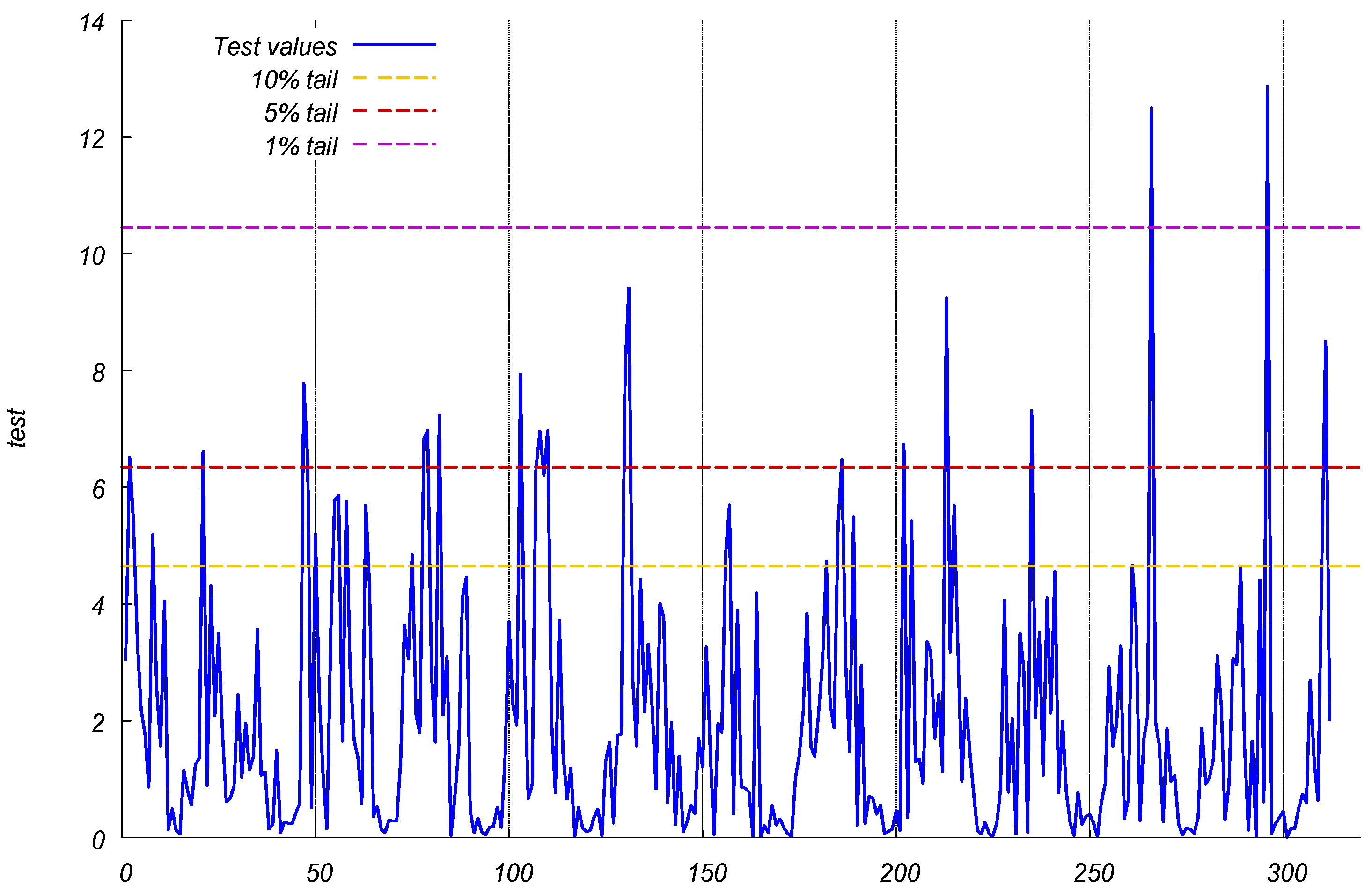
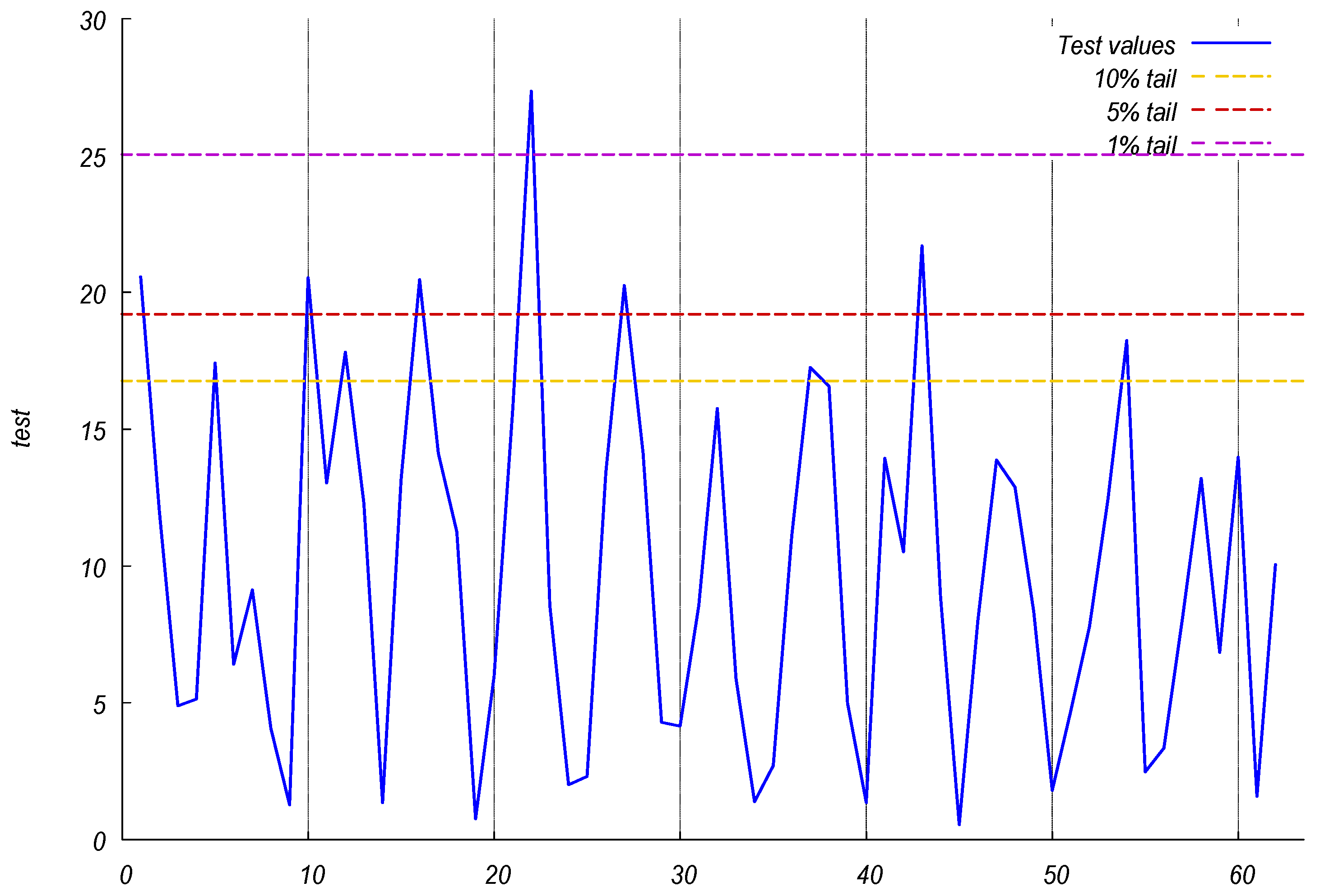
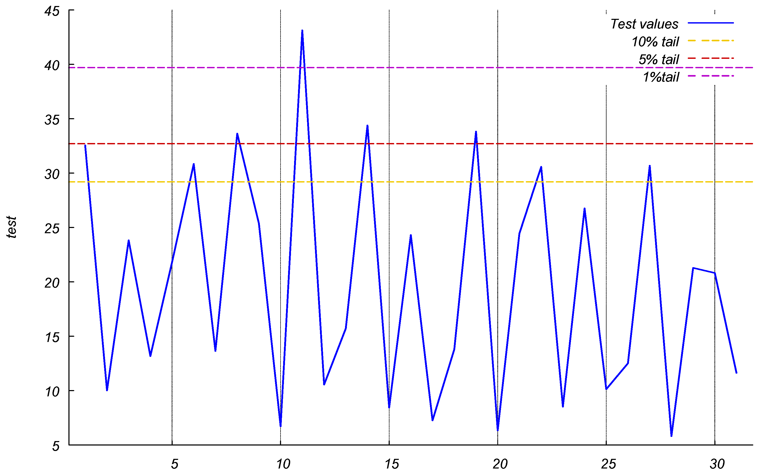
ES and Chi-Squared Intervals
(10%, 5%, 1% Upper Tail Probabilities)
Deg. freedom251020
(A) 10%
Chi-squared4.6059.23615.98728.412
ES4.6509.62716.75829.175
(B) 5%
Chi-squared5.99111.07018.30731.410
ES6.34111.79319.20332.678
(C) 1%
Chi-squared9.21015.08623.20937.566
ES10.44816.55925.03439.683
Notes. Values for the ES test are derived with the estimates reported in (19).
Publisher’s Note: MDPI stays neutral with regard to jurisdictional claims in published maps and institutional affiliations.

