
Anomalous Areas Detection in Rocks Using Time-Difference Adjoint Tomography


Abstract
:1. Introduction
2. Methodology
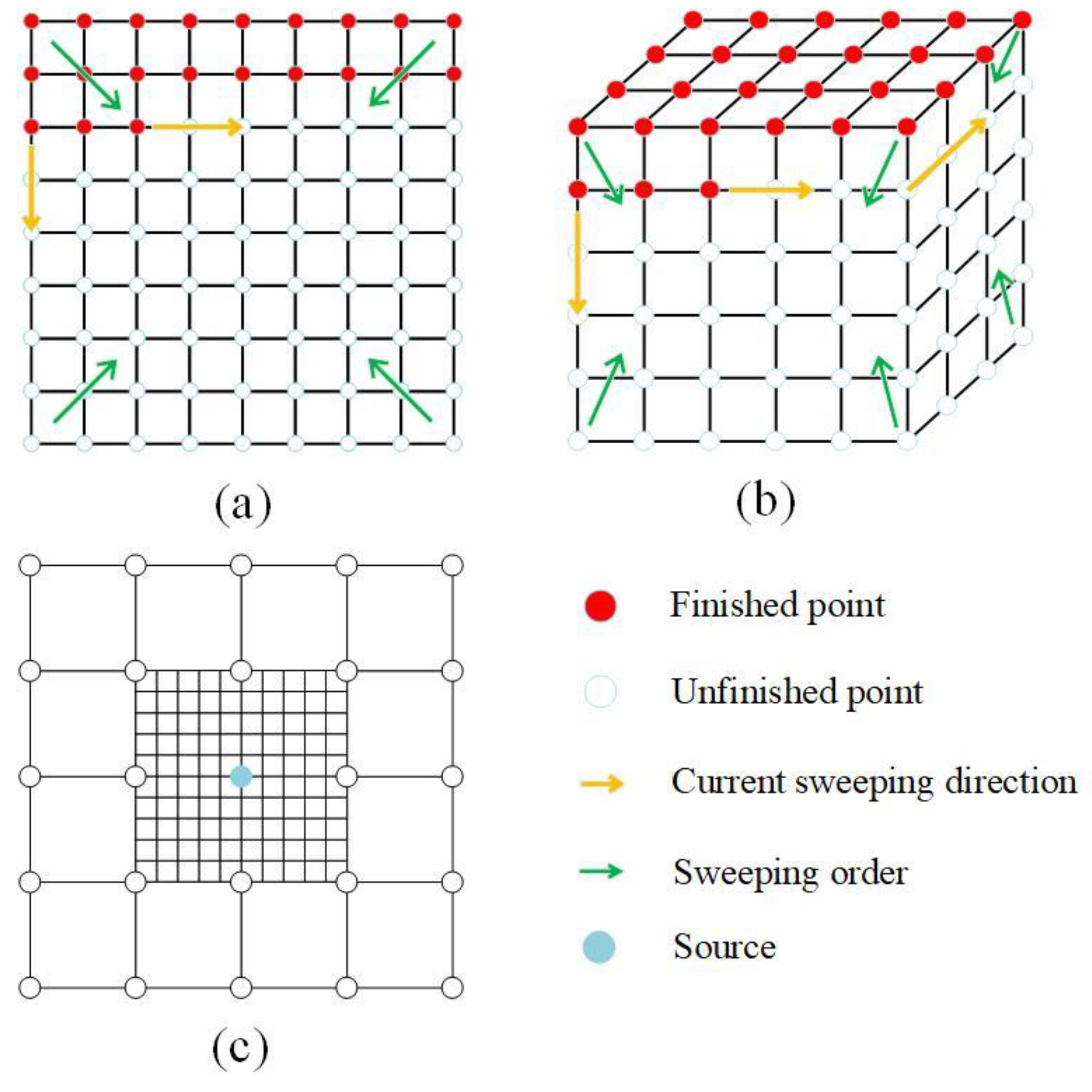
2.1. Model Discretization
2.2. Forward Calculation
2.3. Inversion
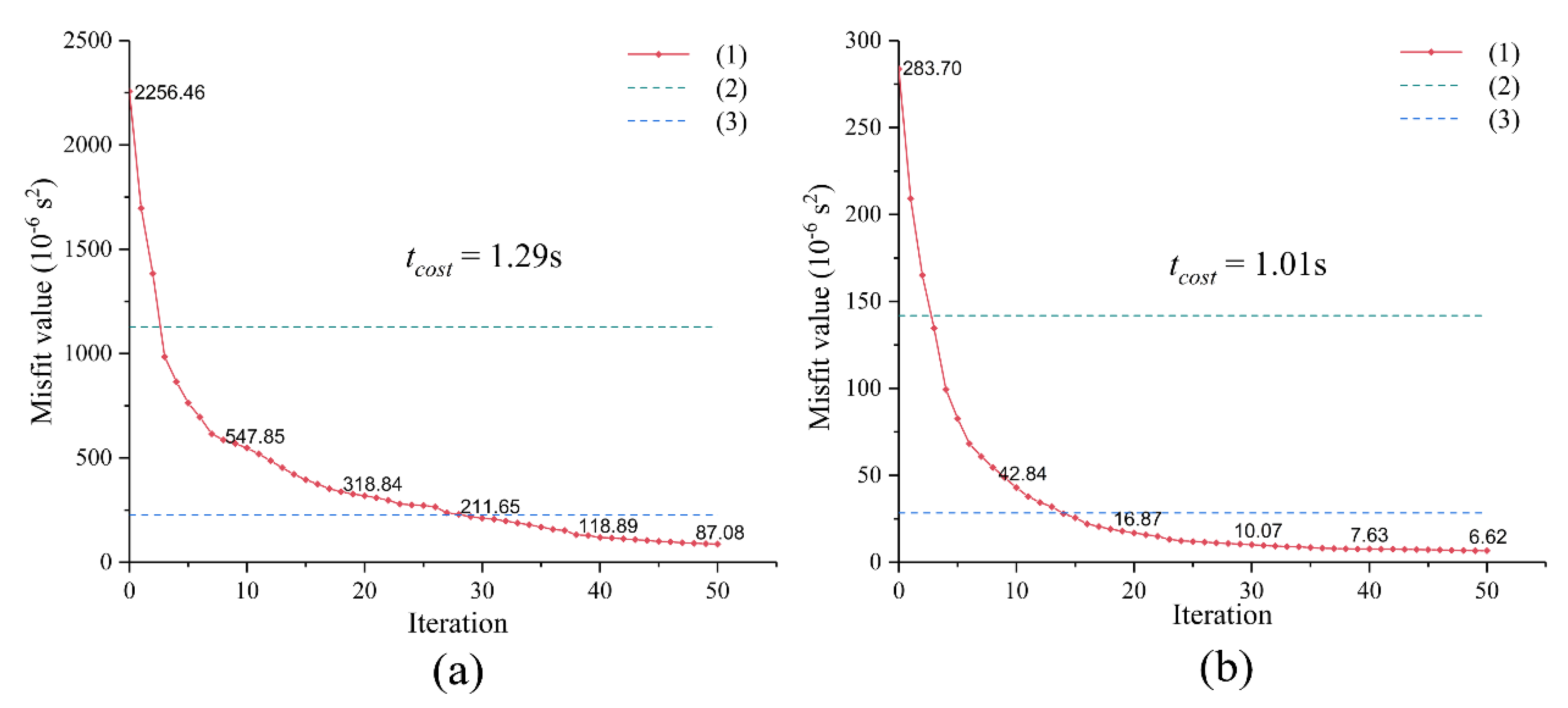
2.3.1. Misfit Function
2.3.2. Model Update
2.3.3. Adjoint Variable and Gradient
2.3.4. Regularization
3. Results and Discussion
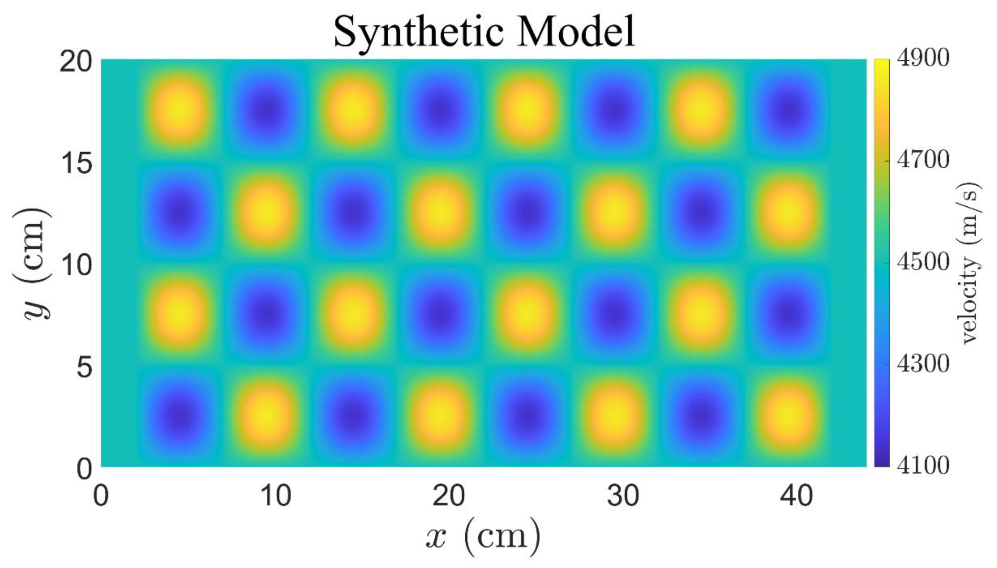
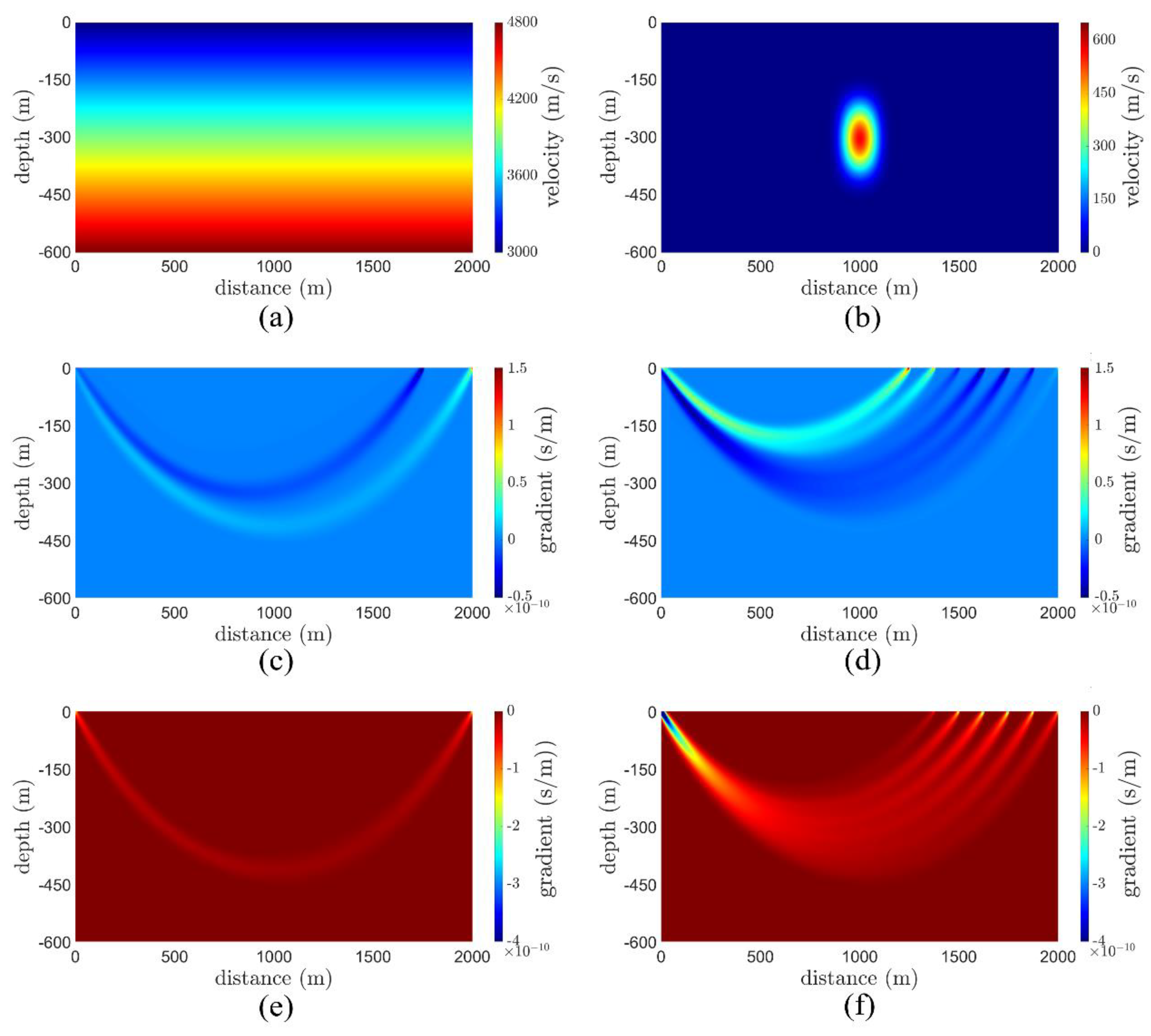
3.1. Numerical Experiments
3.2. Laboratory Case
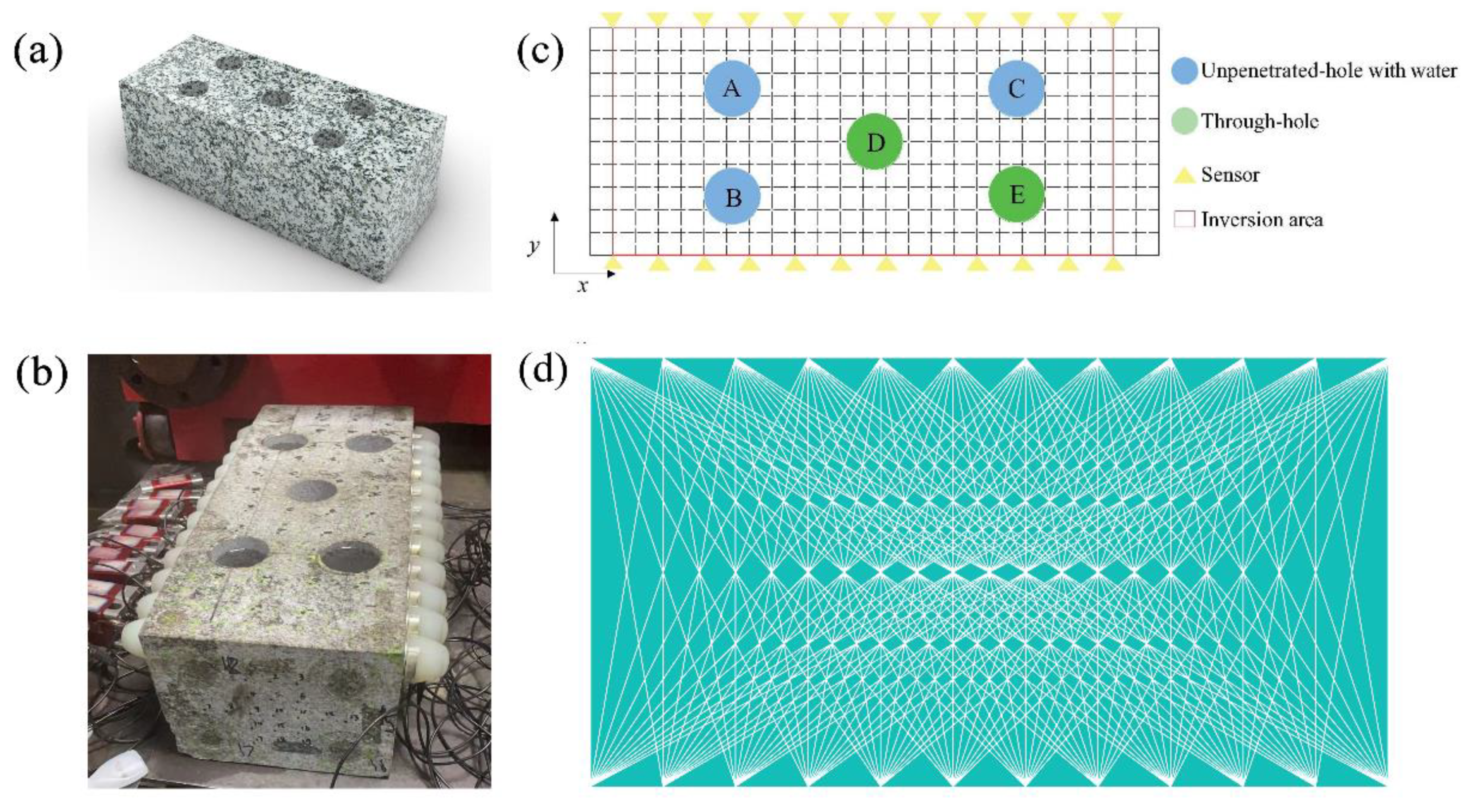
3.2.1. Experimental Overview
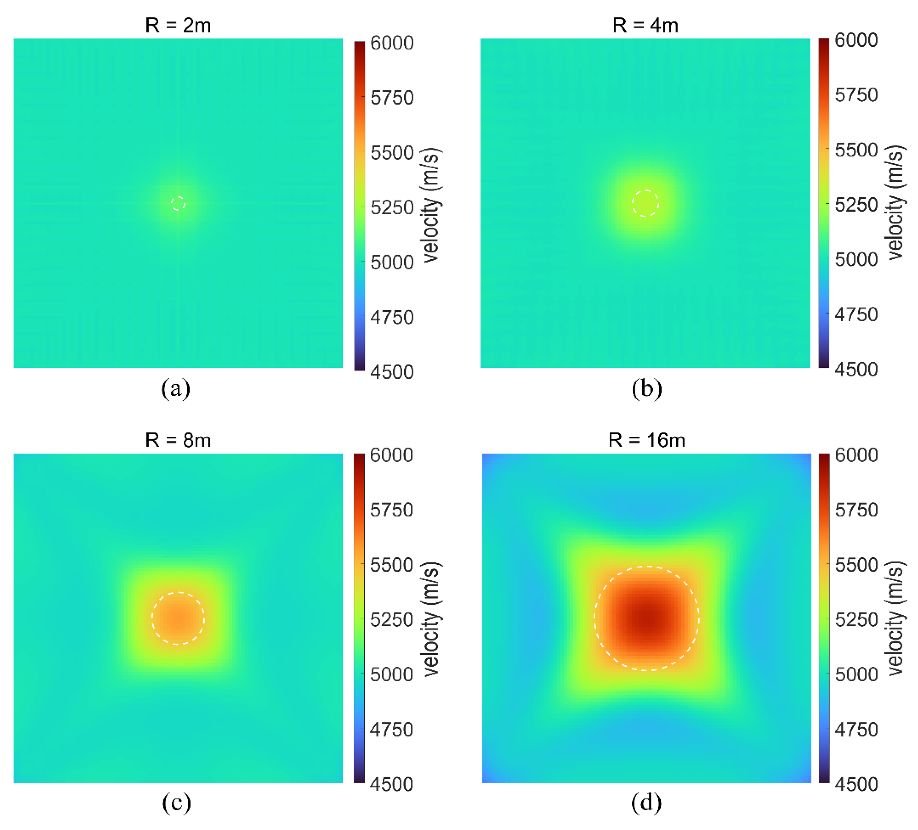
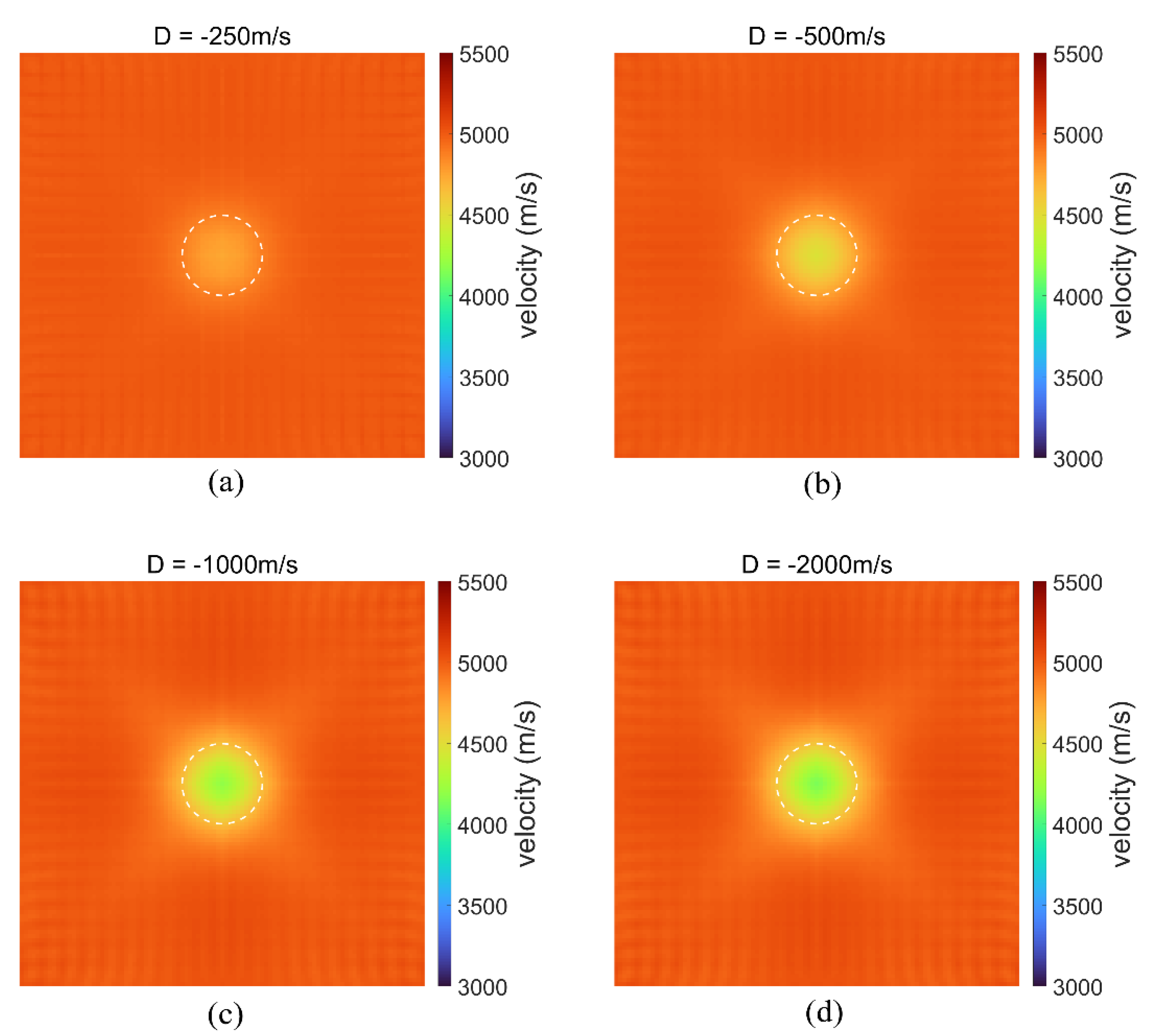
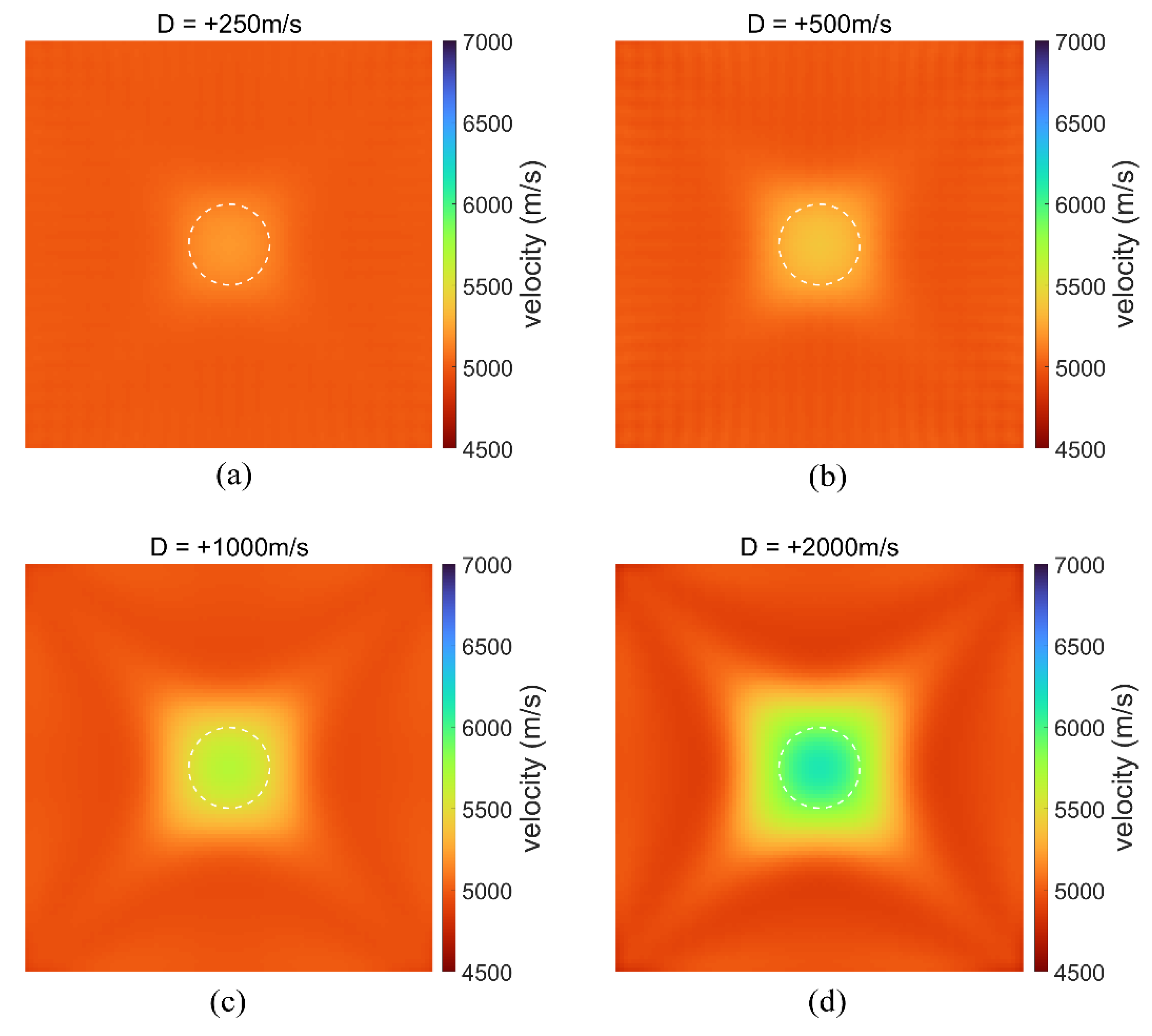
3.2.2. Resolution
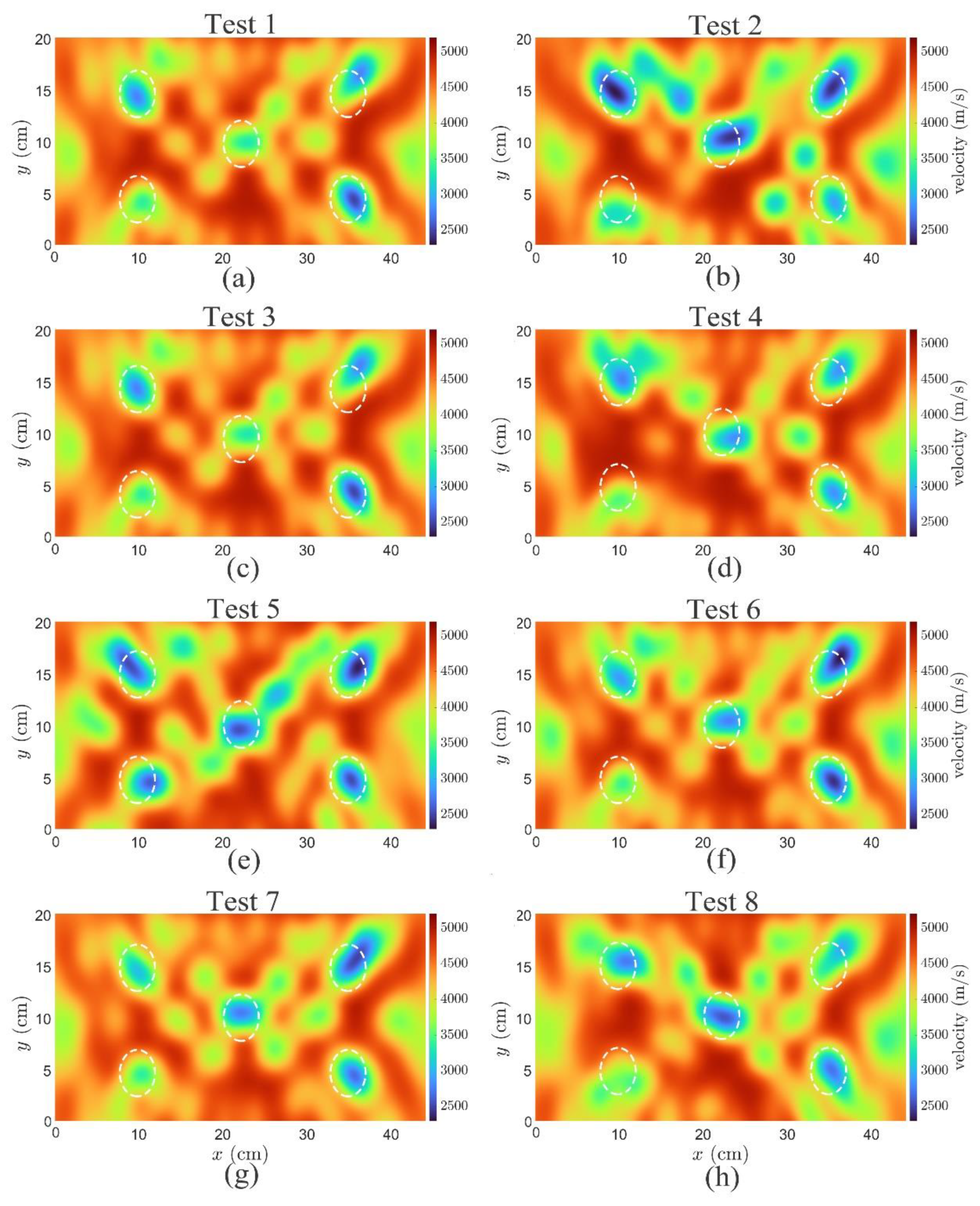
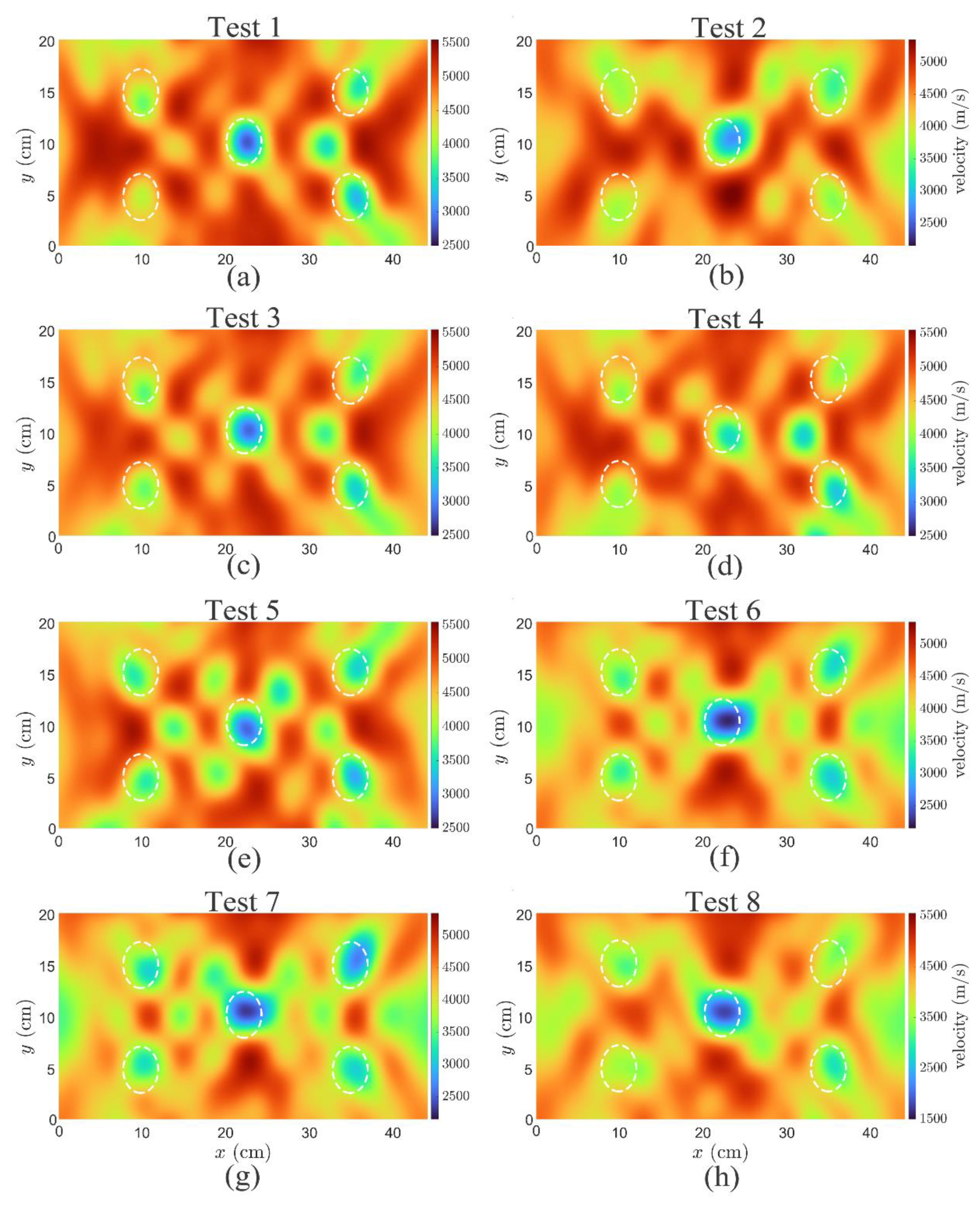
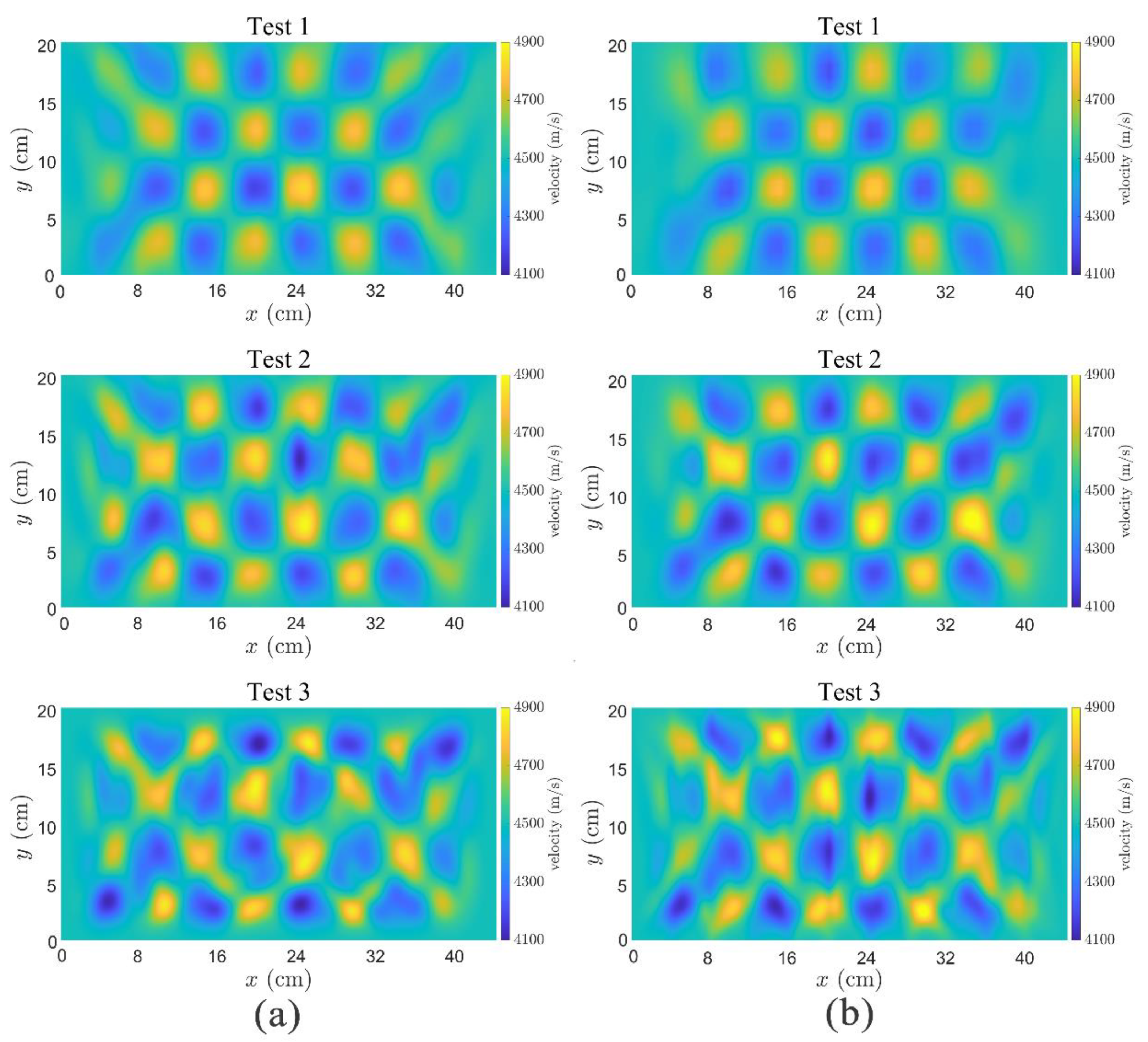
3.2.3. Imaging
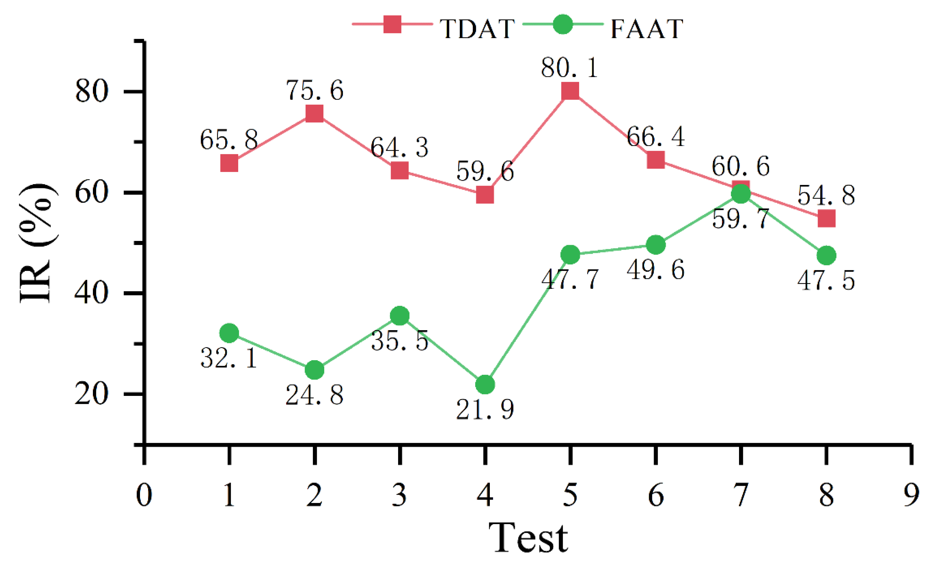
3.2.4. Robustness to Observations
4. Conclusions
Author Contributions
Funding
Institutional Review Board Statement
Informed Consent Statement
Data Availability Statement
Conflicts of Interest
Appendix A. Adjoint Scheme for Time-Difference Tomography
References
- Huang, M.; Ninić, J.; Zhang, Q. BIM, machine learning and computer vision techniques in underground construction: Current status and future perspectives. Tunn. Undergr. Space Technol. 2021, 108, 103677. [Google Scholar] [CrossRef]
- Ma, J.; Dong, L.; Zhao, G.; Li, X. Qualitative method and case study for ground vibration of tunnels induced by fault-slip in underground mine. Rock Mech. Rock Eng. 2019, 52, 1887–1901. [Google Scholar] [CrossRef]
- Yang, G.; Zhang, C.; Min, B.; Chen, W. Complex variable solution for tunneling-induced ground deformation considering the gravity effect and a cavern in the strata. Comput. Geotech. 2021, 135, 104154. [Google Scholar] [CrossRef]
- Sun, Y.; Li, G.; Yang, S. Rockburst Interpretation by a Data-Driven Approach: A Comparative Study. Mathematics 2021, 9, 2965. [Google Scholar] [CrossRef]
- Lv, H.; Wang, D.; Cheng, Z.; Zhang, Y.; Zhou, T. Study on Mechanical Characteristics and Failure Modes of Coal–Mudstone Combined Body with Prefabricated Crack. Mathematics 2022, 10, 177. [Google Scholar] [CrossRef]
- Dong, L.; Chen, Y.; Sun, D.; Zhang, Y. Implications for rock instability precursors and principal stress direction from rock acoustic experiments. Int. J. Min. Sci. Technol. 2021, 31, 789–798. [Google Scholar] [CrossRef]
- Ma, J.; Dong, L.; Zhao, G.; Li, X. Focal Mechanism of Mining-Induced Seismicity in Fault Zones: A Case Study of Yongshaba Mine in China. Rock Mech. Rock Eng. 2019, 52, 3341–3352. [Google Scholar] [CrossRef]
- Dong, L.; Tong, X.; Hu, Q.; Tao, Q. Empty region identification method and experimental verification for the two-dimensional complex structure. Int. J. Rock Mech. Min. Sci. 2021, 147, 104885. [Google Scholar] [CrossRef]
- Dong, L.; Zhang, Y.; Ma, J. Micro-crack mechanism in the fracture evolution of saturated granite and enlightenment to the precursors of instability. Sensors 2020, 20, 4595. [Google Scholar] [CrossRef]
- Dong, L.; Tong, X.; Ma, J. Quantitative investigation of tomographic effects in abnormal regions of complex structures. Engineering 2021, 7, 1011–1022. [Google Scholar] [CrossRef]
- Dong, L.; Tao, Q.; Hu, Q.; Deng, S.; Chen, Y.; Luo, Q.; Zhang, X. Acoustic emission source location method and experimental verification for structures containing unknown empty areas. Int. J. Min. Sci. Technol. 2022; in press. [Google Scholar]
- Lehmann, B.; Orlowsky, D.; Misiek, R. Exploration of tunnel alignment using geophysical methods to increase safety for planning and minimizing risk. Rock Mech. Rock Eng. 2010, 43, 105–116. [Google Scholar] [CrossRef]
- Bürgmann, R. The geophysics, geology and mechanics of slow fault slip. Earth Planet. Sci. Lett. 2018, 495, 112–134. [Google Scholar] [CrossRef] [Green Version]
- Gong, S.Y.; Li, J.; Ju, F.; Dou, L.M.; He, J.; Tian, X.Y. Passive seismic tomography for rockburst risk identification based on adaptive-grid method. Tunn. Undergr. Space Technol. 2019, 86, 198–208. [Google Scholar] [CrossRef]
- Tiberi, C.; Gautier, S.; Ebinger, C.; Roecker, S.; Plasman, M.; Albaric, J.; Déverchère, J.; Peyrat, S.; Perrot, J.; Wambura, R.F.; et al. Lithospheric modification by extension and magmatism at the craton-orogenic boundary: North Tanzania Divergence, East Africa. Geophys. J. Int. 2019, 216, 1693–1710. [Google Scholar] [CrossRef] [Green Version]
- Hosseini, K.; Sigloch, K.; Tsekhmistrenko, M.; Zaheri, A.; Nissen-Meyer, T.; Igel, H. Global mantle structure from multifrequency tomography using P, PP and P-diffracted waves. Geophys. J. Int. 2020, 220, 96–141. [Google Scholar] [CrossRef]
- Chlebowski, D.; Burtan, Z. Geophysical and analytical determination of overstressed zones in exploited coal seam: A case study. Acta Geophys. 2021, 69, 701–710. [Google Scholar] [CrossRef]
- Yordkayhun, S. Geophysical Characterization of a Sinkhole Region: A Study Toward Understanding Geohazards in the Karst Geosites. Sains Malays. 2021, 50, 1871–1884. [Google Scholar] [CrossRef]
- Su, Y.; Dong, L.; Pei, Z. Non-Destructive Testing for Cavity Damages in Automated Machines Based on Acoustic Emission Tomography. Sensors 2022, 22, 2201. [Google Scholar] [CrossRef]
- Aki, K.; Lee, W. Determination of three-dimensional velocity anomalies under a seismic array using first P arrival times from local earthquakes: 1. A homogeneous initial model. J. Geophys. Res. 1976, 81, 4381–4399. [Google Scholar] [CrossRef]
- Glowinski, R.; Leung, S.; Qian, J. A penalization-regularization-operator splitting method for eikonal based traveltime tomography. SIAM J. Imaging Sci. 2015, 8, 1263–1292. [Google Scholar] [CrossRef] [Green Version]
- Jiang, W.; Zhang, J. First-arrival traveltime tomography with modified total-variation regularization. Geophys. Prospect. 2017, 65, 1138–1154. [Google Scholar] [CrossRef]
- Liu, Y.; Wu, Z.; Geng, Z. First-arrival phase-traveltime tomography. Chin. J. Geophys. 2019, 62, 619–633. [Google Scholar]
- Wolfe, C.J. On the mathematics of using difference operators to relocate earthquakes. Bull. Seismol. Soc. Am. 2002, 92, 2879–2892. [Google Scholar] [CrossRef]
- Nolet, G. A breviary of Seismic Tomography; Cambridge University Press: Cambridge, UK, 2008. [Google Scholar]
- Schaeffer, A.; Lebedev, S. Global shear speed structure of the upper mantle and transition zone. Geophys. J. Int. 2013, 194, 417–449. [Google Scholar] [CrossRef]
- Zhang, H.; Thurber, C.H. Double-difference tomography: The method and its application to the Hayward fault, California. Bull. Seismol. Soc. Am. 2003, 93, 1875–1889. [Google Scholar] [CrossRef]
- Waldhauser, F.; Ellsworth, W.L. A double-difference earthquake location algorithm: Method and application to the northern Hayward fault, California. Bull. Seismol. Soc. Am. 2000, 90, 1353–1368. [Google Scholar] [CrossRef]
- Zhang, H.; Thurber, C. Development and applications of double-difference seismic tomography. Pure Appl. Geophys. 2006, 163, 373–403. [Google Scholar] [CrossRef]
- Yang, T.; Westman, E.; Slaker, B.; Ma, X.; Hyder, Z.; Nie, B. Passive tomography to image stress redistribution prior to failure on granite. Int. J. Min. Reclam. Environ. 2015, 29, 178–190. [Google Scholar] [CrossRef]
- Li, J.; Zhang, H.; Rodi, W.L.; Toksoz, M.N. Joint microseismic location and anisotropic tomography using differential arrival times and differential backazimuths. Geophys. J. Int. 2013, 195, 1917–1931. [Google Scholar] [CrossRef] [Green Version]
- Xin, H.; Zhang, H.; Kang, M.; He, R.; Gao, L.; Gao, J. High-resolution lithospheric velocity structure of continental China by double-difference seismic travel-time tomography. Seismol. Res. Lett. 2019, 90, 229–241. [Google Scholar] [CrossRef]
- Yuan, Y.O.; Simons, F.J.; Tromp, J. Double-difference adjoint seismic tomography. Geophys. J. Int. 2016, 206, 1599–1618. [Google Scholar] [CrossRef] [Green Version]
- Virieux, J.; Operto, S. An overview of full-waveform inversion in exploration geophysics. Geophysics 2009, 74, WCC1–WCC26. [Google Scholar] [CrossRef]
- Leung, S.; Qian, J. An adjoint state method for three-dimensional transmission traveltime tomography using first-arrivals. Commun. Math. Sci. 2006, 4, 249–266. [Google Scholar] [CrossRef] [Green Version]
- Zhao, H. A fast sweeping method for eikonal equations. Math. Comput. 2005, 74, 603–627. [Google Scholar] [CrossRef] [Green Version]
- Rouy, E.; Tourin, A. A viscosity solutions approach to shape-from-shading. SIAM J. Numer. Anal. 1992, 29, 867–884. [Google Scholar] [CrossRef]
- Plessix, R.E. A review of the adjoint-state method for computing the gradient of a functional with geophysical applications. Geophys. J. Int. 2006, 167, 495–503. [Google Scholar] [CrossRef]
- Liu, Y.; Tong, P. Eikonal equation-based P-wave seismic azimuthal anisotropy tomography of the crustal structure beneath northern California. Geophys. J. Int. 2021, 226, 287–301. [Google Scholar] [CrossRef]
- Sei, A.; Symes, W.W. Gradient calculation of the traveltime cost function without ray tracing. In SEG Technical Program Expanded Abstracts 1994; Society of Exploration Geophysicists: Tulsa, OK, USA, 1994; pp. 1351–1354. [Google Scholar]
- Taillandier, C.; Noble, M.; Chauris, H.; Calandra, H. First-arrival traveltime tomography based on the adjoint-state method. Geophysics 2009, 74, WCB1–WCB10. [Google Scholar] [CrossRef]
- Qian, J.; Symes, W.W. An adaptive finite-difference method for traveltimes and amplitudes. Geophysics 2002, 67, 167–176. [Google Scholar] [CrossRef] [Green Version]


| Test | Inversion Area/cm | Grid Length/cm | Number of Grids | Number of Iterations |
|---|---|---|---|---|
| 1 | 44 × 20 | 1 | 44 × 20 | 30 |
| 2 | 0.5 | 88 × 44 | ||
| 3 | 0.25 | 176 × 80 |
| Test | System Error/μs | Random Gaussian Noise/μs | Number of Iterations | |
|---|---|---|---|---|
| Mean | Standard Deviation | |||
| 1 | +4 | 0 | 0 | 50 |
| 2 | 0 | 1.00 | ||
| 3 | +3 | 0.25 | ||
| 4 | +3 | 0.50 | ||
| 5 | +3 | 0.75 | ||
| 6 | −3 | 0.25 | ||
| 7 | −3 | 0.50 | ||
| 8 | −3 | 0.75 | ||
Publisher’s Note: MDPI stays neutral with regard to jurisdictional claims in published maps and institutional affiliations. |
© 2022 by the authors. Licensee MDPI, Basel, Switzerland. This article is an open access article distributed under the terms and conditions of the Creative Commons Attribution (CC BY) license (https://creativecommons.org/licenses/by/4.0/).
Share and Cite
Wang, F.; Xie, X.; Pei, Z.; Dong, L. Anomalous Areas Detection in Rocks Using Time-Difference Adjoint Tomography. Mathematics 2022, 10, 1069. https://doi.org/10.3390/math10071069
Wang F, Xie X, Pei Z, Dong L. Anomalous Areas Detection in Rocks Using Time-Difference Adjoint Tomography. Mathematics. 2022; 10(7):1069. https://doi.org/10.3390/math10071069
Chicago/Turabian StyleWang, Feiyue, Xin Xie, Zhongwei Pei, and Longjun Dong. 2022. "Anomalous Areas Detection in Rocks Using Time-Difference Adjoint Tomography" Mathematics 10, no. 7: 1069. https://doi.org/10.3390/math10071069
APA StyleWang, F., Xie, X., Pei, Z., & Dong, L. (2022). Anomalous Areas Detection in Rocks Using Time-Difference Adjoint Tomography. Mathematics, 10(7), 1069. https://doi.org/10.3390/math10071069