On Primitive Recursive Characteristics of Chess

Abstract

Several characteristics of chess are investigated with methods of computability and number theories. It is shown that for an unfinished game it is primitive recursively decidable whether the game is winnable, drawable, or absolutely losable within a specified number of future moves for the player whose turn it is to play on the last board of the game. It is also shown that there exist primitive recursive procedures to compute optimal continuations of unfinished games within specified numbers of future moves and that the set of chess games is recursive.

1. Introduction

A deterministic two-player board game (D2PBG) is played by two players on a finite board. The board is finite in the sense that it contains finitely many positions where each player can make a move. The players take turns making moves on the board with exactly one move per player per turn. The order of turns is pre-determined and cannot be changed at any point during the game. At each turn, a move is chosen by a player out of finitely many possible moves and uniquely determines the next board.

A D2PBG is a sequence of boards with a unique starting board. The last board (or the end board) of any such sequence is reached from the starting board after finitely many valid (i.e., allowed by the rules of the game) moves, and can be classified as a win for either player, a draw, or an unfinished board in the sense that the game can continue from its end board for a positive number of moves into the future. Examples of D2PBGs are Tic Tac Toe [1] and numerous variants thereof (e.g., Qubic [2]), chess, and checkers.

We follow Kleene’s classification of computational methods into decision procedures and calculation procedures (Chapter 6 in [3]). A decision procedure is a mechanical method expressed in a symbolic formalism (e.g., $\lambda$-calculus [4] or the language L [5]) that returns, in finitely many steps, a positive (e.g., 1) or negative (e.g., 0) answer to a class of problems. We refer to such classes of problems as characteristics. Thus, the characteristic of relative primality of two positive integers in number theory is decidable by a decision procedure that uses Euclid’s algorithm to find their greatest common divisor, checks whether it is equal to 1 and returns 1 (i.e., true) if it is, and 0 (i.e., false) if it is not. The characteristic of winnability in the game of Tic Tac Toe is decidable by a decision procedure that for the end board b of any unfinished Tic Tac Toe game returns 1 if it is winnable by either player (i.e., X or O) whose turn it is to play on b within M moves where M is a positive integer [6] and returns 0 if it is not winnable. As shown in this investigation, the characteristic of stalemate for a chess game is decidable by a decision procedure that determines if the end board of the game is a stalemate for the player whose turn it is to play on it. We refer to a feature of a D2PBG as a decision characteristic if there exists a decision procedure to decide it.

A calculation procedure requires an effective (i.e., mechanical and deterministic) construction, in finitely many steps, of a mathematical object (e.g., a sequence of instructions in $\lambda$-calculus, a plot, a matrix, etc.) that satisfies specific properties. Euclid’s algorithm is a calculation procedure for the characteristic of relatively primality, because it constructs in finitely many steps the required object – the greatest common divisor of two numbers. Similarly, a calculation procedure for the game of Tic Tac Toe takes any unfinished game and, if the latter is winnable within M moves by the player whose turn it is to play on its last board, constructs a sequence of at most M moves that result in a win board for the player. We call a feature of a D2PBG a calculation characteristic if there exists a calculation procedure to produce required mathematical objects (e.g., boards or games) with specific properties. The existence of a calculation procedure for a characteristic implies the existence of a decision procedure for it that returns 1 if a required object is constructed and 0 otherwise.

We may require that a decision or calculation procedure itself satisfy certain properties. In general, those properties can be either structural (e.g., a procedure must be primitive recursive, computable, or partially computable) or algorithmic (e.g., the number of steps the procedure takes to return a decision or construct an object must be the function of the size of the input n such as $O\left(n^3\right)$ and must be known ahead of the calculation).

In this article, we focus on the structural (and, more specifically, primitive recursive) characteristics of chess. In that, we follow a fundamental tenet of classical computability theory, which, as formulated by Rogers [4], states that

‘‘[w]e thus require that a computation

terminate after some finite number

of steps; we do not insist on an a

priori ability to estimate this number.’’

We thus study the arithmetization of chess (and, by implication, of other D2PBGs) to analyze the game’s characteristics with methods of number theory and classical computability. If a decision characteristic of chess can be computed with a primitive recursive predicate, we call the characteristic primitive recursively decidable or pr-decidable; if a calculation characteristic of chess can be computed with a primitive recursive function, we refer to it as primitive recursively computable or pr-computable.

Unfortunately, the theory of recursive functions appears to lack a uniform, commonly accepted formalism. The treatment of primitive recursive functions in this article is based on the formalism by Davis et al. in [5], which, in turn, is based on Kleene’s formalism in (Chapter 9 in [3]). Alternative treatments are given in [7], where primitive recursive functions are formalized as loop programs consisting of assignment and iteration statements similar to DO statements in FORTRAN, or in [4], where primitive recursive functions are described with $\lambda$-calculus.

The words number or numbers in this article refer to a natural number or natural numbers, respectively, where the set of natural number is defined as $\mathbb{N}=\{0,1,2,\dots \}$. All small letters (e.g., x, y, z, a, b, c, i, j, k, t, l, m, n, u, z, $\zeta$, etc.) with appropriate numeric or symbolic subscripts (when the latter are required by the context) are variables that denote numbers. We sometimes use capital letters (e.g., M, Z) with suitable subscripts or no subscripts to refer to numbers that we believe are significant for the current exposition.

In this article, all functions map ${\mathbb{N}}^j$ to ${\mathbb{N}}^k$ (i.e., ${\mathbb{N}}^j\mapsto {\mathbb{N}}^k$), where j and k are positive numbers. We use the symbol ≡ to define predicates (e.g., $P(x_1,x_2)\equiv x_1<x_2$). We use the capital letter P with prime superscripts (e.g., $P^{\prime }$) or numeric subscripts to define predicates and use the capital letter F with numeric subscripts to define functions. Number 0 when referencing the value of a predicate means that the predicate is false; number 1 when referencing the value of a predicate means that the predicate is true.

When the argument variables of a function or predicate are clear from the context, we use the notation $P(·)$ or $F(·)$ for brevity. For example, $P(·)$ instead of $P(x_1,x_2)$ and $F(·)$ instead of $F(x_1,x_2,x_3)$.

When a variable occurs free in the definition of a predicate or a function it refers to a number referenced in the immediate context. For example, let $z=10$ and let $P\left(d\right)\equiv 2^d|(z+1)$. In this definition of $P(·)$, z refers to number 10.

In defining some predicates, we occasionally abbreviate Boolean combinations of numerical predicates. For example, $i\le j\wedge j\le k$ is abbreviated as $i\le j\le k$; $i\ge j\wedge j\ge k$ as $i\ge j\ge k$; $i=j\wedge j=k$ as $i=j=k$, etc.

The remainder of the article is organized as follows. In Section 2, several functions are defined that are shown to be primitive recursive in [5]. In Section 3, we use the primitive recursive functions in Section 2 to define several primitive recursive functions to manipulate Gödel numbers (G-numbers). We call these functions G-number operators and use them in Section 4 to show several characteristics of chess and to be pr-decidable and pr-computable. In Section 6 and Section 7, we discuss and summarize our findings.

2. Preliminaries

Let $f(x_1,\dots ,x_k)$ be a function and $g_1,\dots ,g_k$ be functions, where each $g_i$, $1\le i\le k$, is a function of n arguments. Then $h(x_1,\dots ,x_n)$ is obtained by composition from $f,g_1,\dots ,g_k$ if

$$h(x_1,\dots ,x_n)=f(g_1(x_1,\dots ,x_n),\dots ,g_k(x_1,\dots ,x_n)).$$

(1)

Let $k\in \mathbb{N}$ and $\varphi (x,y):{\mathbb{N}}^2\mapsto \mathbb{N}$ be total. Let $f(x_1,\dots ,x_n):{\mathbb{N}}^n\mapsto \mathbb{N}$ and $g(x_1,\dots ,x_{n+2}):{\mathbb{N}}^{n+2}\mapsto \mathbb{N}$ be total. If h is obtained from $\varphi$ by the recurrences in (2) or from f and g by the recurrences in (3), then h is obtained from $\varphi$ or from f and g by primitive recursion or, simply, by recursion.

$$\begin{array}{ccc}h\left(0\right)\hfill & =\hfill & k,\hfill \\ h(t+1)\hfill & =\hfill & \varphi (t,h(t\left)\right)\hfill \end{array}$$

(2)

$$\begin{array}{ccc}h(x_1,\dots ,x_n,0)\hfill & =\hfill & f(x_1,\dots ,x_n),\hfill \\ h(x_1,\dots ,x_n,t+1)\hfill & =\hfill & g(t,h(x_1,\dots ,x_n,t),x_1,\dots ,x_n)\hfill \end{array}$$

(3)

Let

$$\begin{array}{ccc}\hfill & s\left(x\right)=x+1;\hfill & \\ \hfill & n\left(x\right)=0;\hfill & \\ \hfill & u_i^n(x_1,···,x_n)=x_i,\hfill & 1\le i\le n,\hfill \end{array}$$

(4)

be the three initial functions. A function is primitive recursive if it can be obtained from the initial functions by a finite number of applications of composition or recursion as defined in (1)–(3) [5].

A total function $P(x_1,\dots ,x_n)$ is a predicate if for any n numbers $y_1,\dots ,y_n$ $P(y_1,\dots ,y_n)=1$ or $P(y_1,\dots ,y_n)=0$, where 1 designates true and 0 false. The expression ${(\exists t)}_{\le z}$ is a bounded existential quantifier so that if $P(t,x_1,\dots ,x_n)$ is a predicate, ${(\exists t)}_{\le z}P(t,x_1,\dots ,x_n)=1$, if $P(t,x_1,\dots ,x_n)=1$, for at least one t such that $0\le t\le z$. The expression ${(\exists t)}_{\le z}P(t,x_1,\dots ,x_n)$ is called the bounded existential quantification of $P(·)$.

The expression ${(\forall t)}_{\le z}$ is a bounded universal quantifier so that, if $P(t,x_1,\dots ,x_n)$ is a predicate, then ${(\forall t)}_{\le z}P(t,x_1,\dots ,x_n)=1$, if $P(t,x_1,\dots ,x_n)=1$, for every t such that $0\le t\le z$. The expression ${(\forall t)}_{\le z}P(t,x_1,\dots ,x_n)$ is called the bounded universal quantification of $P(·)$.

If $P(t,x_1,\dots ,x_n)$ is a predicate and z is a number, then

$$y={\displaystyle \underset{t\le z}{\min }}P(t,x_1,\dots ,x_n)$$

is called the bounded minimalization of $P(·)$ and defines the smallest number $0\le t\le z$ for which the predicate $P(·)$ is true or 0 if there is no such number. If

$${\displaystyle \underset{t\le z}{\min }}P(t,x_1,\dots ,x_n)=0$$

and $P(0,x_1,\dots ,x_n)=1$, then 0 returned by the bounded minimalization of $P(·)$ is the smallest number $\le z$ for which $P(·)$ holds. If $P(0,x_1,\dots ,x_n)=0$, then 0 returned by the minimalization of $P(·)$ means that there is no number $0\le t\le z$, for which $P(t,x_1,\dots ,x_n)$ holds. If this additional check on 0 must be avoided in a given context, t in the minimalized predicate $P(·)$ must be required to be greater than 0 (e.g., $P(t,x_1,x_2)\equiv t\le x_1·x_2\wedge t>0$), in which case, 0 returned by the minimalization of $P(·)$ means that there is no $0\le t\le z$ for which $P(·)$ holds. The operator min is similar to Kleene’s operator $\mu$ [3]. If $P(x_1,\dots ,x_n)$ is a n-ary predicate, we occasionally write $P(x_1,\dots ,x_n)$ to abbreviate $P(x_1,\dots ,x_n)=1$ and write $\neg P(x_1,\dots ,x_n)$ to abbreviate $P(x_1,\dots ,x_n)=0$.

It is shown in [5] that 1) the predicates $x=y$, $x\ne y$, $x<y$, $x>y$, $x\le y$, $x\ge y$, and $x|y$ (x divides y or x is a divisor of y) are primitive recursive; 2) any Boolean combination of primitive recursive predicates is primitive recursive; and 3) if a predicate $P(·)$ is primitive recursive, then so are its negation and its bounded minimalization and bounded universal and existential quantifications. We will use the notation $x\nmid y$ to denote $\neg \left\{x\right|y\}$ (i.e., x does not divide y or x is not a divisor of y).

Let $x\dot{-}$ y = x − y$,if$ x ≥ 0, and x ∸ y = 0$,\mathrm{if}$ x < y. Thefunction x ∸ y is shown to be primitive recursive in [5]. Let the pairing of numbers x and y be defined as

$$\begin{array}{ccc}\hfill & \langle x,y\rangle =z,\hfill & \end{array}$$

(5)

where

$$\begin{array}{l}z=2^x(2y+1)\dot{-}1\\ \gamma (d)\equiv \{2^d|(z+1){\wedge (\forall c)}_{\le (z+1)}\{2^c\nmid (z+1)\vee c\le d\}\};\hfill \\ x=\underset{d\le z+1}{\min }\gamma (d);\\ y=\frac{1}{2}(\frac{z+1}{2^x}\dot{-}1).\end{array}$$

The minimalization of the primitive recursive predicate $\gamma (·)$ above makes x the largest number such that $2^x|(z+1)$. As shown in [5], for any number z, there are unique x and y such that $\langle x,y\rangle =z$ and the pairing function $\langle x,y\rangle$ is primitive recursive. For example, if $z=27$, then

$$\begin{array}{l}x=\underset{d\le 28}{\min }\gamma (d)=2;\\ y=\frac{1}{2}(\frac{28}{2^2}\dot{-}1)=3;\\ \langle 2,3\rangle =2^2(2·3+1)\dot{-}1=27.\end{array}$$

Let the functions $l\left(z\right)$ and $r\left(z\right)$ in (6) return the left and right components of any number z. Since the predicate $z=\langle x,y\rangle$ is primitive recursive, both

$$\begin{array}{cc}\hfill l\left(z\right)& ={\displaystyle \underset{x\le z}{\min }}\left\{{(\exists y)}_{\le z}\{z=\langle x,y\rangle \}\right\}\hfill \\ \\ \hfill r\left(z\right)& ={\displaystyle \underset{y\le z}{\min }}\left\{{(\exists x)}_{\le z}\{z=\langle x,y\rangle \}\right\}\hfill \end{array}$$

(6)

are primitive recursive, because they are bounded minimalizations of the bounded existential quanitifcations of primitive recursive predicates. Thus, if $z=27=\langle 2,3\rangle$, then $l\left(z\right)=2$, $r\left(z\right)=3$, and, in general, $\langle l\left(z\right),r\left(z\right)\rangle =z$ for any number z.

Let $p_n$ be the n-th prime so that $p_1=2$, $p_2=3$, $p_3=5$, etc. Let $p_0=0$, by default. In [5], $p_n$ is shown to be computed by a primitive recursive function, which we define as

$$\pi \left(i\right)=p_i.$$

(7)

Thus, $\pi \left(0\right)=0$, $\pi \left(1\right)=2$, $\pi \left(2\right)=3$, $\pi \left(3\right)=5$, $\pi \left(4\right)=7$, $\pi \left(5\right)=11$, etc.

Let $(a_1,\dots ,a_n)$ be a sequence of numbers. The function in (8) computes the Gödel number (G-number) of this sequence.

$$[a_1,\dots ,a_n]=\prod _{i=1}^n\pi {\left(i\right)}^{a_i}$$

(8)

The function $[a_1,\dots ,a_n]$ is shown to be primitive recursive in [5], because $x·y$, $x^y$, $\pi \left(i\right)$ are primitive recursive, and a finite product of primitive recursive functions is, by induction, primitive recursive. The G-number of the empty number sequence $\left(\right)$ is 1. Thus, the G-number of $(3,101,7891,1,43)$ is

$$\begin{array}{ccc}[3,101,7891,1,43]\hfill & =\hfill & 2^3·3^{101}·5^{7891}·7^1·{11}^{43}.\hfill \end{array}$$

Let $x=[a_1,\dots ,a_n]$. The accessor function ${\left(x\right)}_i=a_i$ in (9), which returns the i-th element of x, is shown to be primitive recursive in [5].

$${\left(x\right)}_i={\displaystyle \underset{t\le x}{\min }}\{\pi {\left(i\right)}^{t+1}\nmid x\}$$

(9)

The function ${\left(x\right)}_i$ allows us to treat G-numbers as arrays (i.e., sequences of numbers). Thus, if $x=[1,7,13]$, then

$$\begin{array}{ccc}{\left(x\right)}_1\hfill & =\hfill & 1;\hfill \\ {\left(x\right)}_2\hfill & =\hfill & 7;\hfill \\ {\left(x\right)}_3\hfill & =\hfill & 13;\hfill \\ {\left(x\right)}_j\hfill & =\hfill & 0,\mathrm{if}j>3.\hfill \end{array}$$

Since G-numbers are sequences, they have lengths. Thus, if $x=[a_1,a_2,\dots ,a_n]$, the length of x is the position of the last non-zero prime power in x and is computed by the primitive recursive function $\mathtt{L}\mathtt{t}(·)$ in (10). We note that $\mathtt{L}\mathtt{t}\left([a_1,\dots ,a_n]\right)=n$ if and only if $a_n\ne 0$, and if $\mathtt{L}\mathtt{t}\left(x\right)=n$, then $[{\left(x\right)}_1,\dots ,{\left(x\right)}_n]=x$.

$$\mathtt{L}\mathtt{t}\left(x\right)={\displaystyle \underset{i\le x}{\min }}\{{\left(x\right)}_i\ne 0\wedge {(\forall j)}_{\le x}\{j\le i\vee {\left(x\right)}_j=0\}\}$$

(10)

Thus,

$$\mathtt{L}\mathtt{t}\left(540\right)=\mathtt{L}\mathtt{t}\left(\right[2,3,1\left]\right)=3.$$

The function $x/y$ that returns the integer part of the quotient $x/y$ is shown to be primitive recursive in [5]. Thus, $\lfloor 7/2\rfloor =3$; $\lfloor 2/5\rfloor =0$; $\lfloor 8/5\rfloor =1$, and $\lfloor x/0\rfloor =0$ for any number x.

3. G-Number Operators

In this section, we define several primitive recursive functions on G-numbers. We call these functions G-number operators and use them in Section 4 to show that several characteristics of chess and are pr-decidable and pr-computable.

3.1. Assignment

Let

$$P_0(i,b)\equiv 1\le i\le \mathtt{L}\mathtt{t}\left(b\right)\wedge b\ge 1.$$

The function

$$\mathtt{s}\mathtt{e}\mathtt{t}(b,i,v)=\left\{\begin{array}{cc}\lfloor \frac{b}{\pi {\left(i\right)}^{{\left(b\right)}_i}}\rfloor ·\pi {\left(i\right)}^v\hfill & \mathrm{if}{P}_0(i,b),\hfill \\ \\ 0\hfill & \mathrm{otherwise}\hfill \end{array}\right.$$

(11)

assigns the value of the i-th element of b to v. By Theorem 5.4 (the Definition by Cases Theorem) of Chapter 3 in [5] (which we henceforth abbreviate as the DCT), $\mathtt{s}\mathtt{e}\mathtt{t}(·)$ in (11) is primitive recursive, because $P_0(·)$ is primitive recursive. Thus, if $b=[1,2]=2^1{3}^2=18$, $i=1$, and $v=3$, then

$$\mathtt{s}\mathtt{e}\mathtt{t}([1,2],1,3)=\lfloor \frac{b}{\pi {\left(1\right)}^{{\left(b\right)}_1}}\rfloor ·\pi {\left(1\right)}^3=$$

$$\lfloor \frac{[1,2]}{2^{{\left([1,2]\right)}_1}}\rfloor ·2^3=\lfloor \frac{2^1·3^2}{2^1}\rfloor ·2^3=[3,2]=72$$

or, more succinctly,

$$\mathtt{s}\mathtt{e}\mathtt{t}(18,1,3)=72.$$

If $b=72$, $i=2$, and $v=4$, then

$$\mathtt{s}\mathtt{e}\mathtt{t}(72,2,4)=648,$$

because

$$\mathtt{s}\mathtt{e}\mathtt{t}\left(\mathtt{s}\mathtt{e}\mathtt{t}\right(18,1,3),2,4)=\mathtt{s}\mathtt{e}\mathtt{t}(72,2,4)=$$

$$\lfloor \frac{72}{3^2}\rfloor ·3^4=[3,4]=648.$$

If $b=[2,3,5,8,13]$ $i=5$, $v=21$, then

$$\begin{gathered} \mathtt{s}\mathtt{e}\mathtt{t}(b,5,21)=\lfloor \frac{b}{{11}^{13}}\rfloor {11}^{21}=[2,3,5,8,21]= \\ 14398076794131917643247179978712500 \end{gathered}$$

or, more succinctly,

$$\begin{array}{l}\mathtt{s}\mathtt{e}\mathtt{t}(67168090852890380796712500,5,21)=\\ 14398076794131917643247179978712500.\end{array}$$

3.2. Count

Let

$$\begin{array}{ccc}\mathtt{c}\mathtt{n}\mathtt{t}\mathtt{x}(x,y,0)\hfill & =\hfill & 0,\hfill \\ \mathtt{c}\mathtt{n}\mathtt{t}\mathtt{x}(x,y,t+1)\hfill & =\hfill & F_0(x,y,t,\mathtt{c}\mathtt{n}\mathtt{t}\mathtt{x}(x,y,t)),\hfill \end{array}$$

where

$$F_0(x,y,t,c)=\left\{\begin{array}{cc}1+c\hfill & \mathrm{if}{\left(y\right)}_{s\left(t\right)}=x,\hfill \\ c\hfill & \mathrm{otherwise}.\hfill \end{array}\right.$$

The function $F_0(·)$ is primitive recursive by the DCT. Therefore, the function $\mathtt{c}\mathtt{n}\mathtt{t}\mathtt{x}(·)$ is primitive recursive, because it is obtained from $s\left(x\right)$ and $F_0(·)$ by composition and recursion. The function $\mathtt{c}\mathtt{n}\mathtt{t}(·)$ in (12) to compute the count of occurrences of x in y is also primitive, because it is obtained by composition from $\mathtt{c}\mathtt{n}\mathtt{t}\mathtt{x}(·)$ and $\mathtt{L}\mathtt{t}\left(x\right)$.

$$\mathtt{c}\mathtt{n}\mathtt{t}(x,y)=\mathtt{c}\mathtt{n}\mathtt{t}\mathtt{x}(x,y,\mathtt{L}\mathtt{t}(y\left)\right)$$

(12)

Let y = 30,870 = [1, 2, 1, 3]. Then

$$\begin{array}{ccccc}\mathtt{c}\mathtt{n}\mathtt{t}(1,y)\hfill & =\hfill & \mathtt{c}\mathtt{n}\mathtt{t}\mathtt{x}(1,y,4)\hfill & & \\ & =\hfill & F_0(1,y,3,\mathtt{c}\mathtt{n}\mathtt{t}\mathtt{x}(1,y,3));\hfill & & \\ \mathtt{c}\mathtt{n}\mathtt{t}\mathtt{x}(1,y,3)\hfill & =\hfill & F_0(1,y,2,\mathtt{c}\mathtt{n}\mathtt{t}\mathtt{x}(1,y,2));\hfill & & \\ \mathtt{c}\mathtt{n}\mathtt{t}\mathtt{x}(1,y,2)\hfill & =\hfill & F_0(1,y,1,\mathtt{c}\mathtt{n}\mathtt{t}\mathtt{x}(1,y,1));\hfill & & \\ \mathtt{c}\mathtt{n}\mathtt{t}\mathtt{x}(1,y,1)\hfill & =\hfill & F_0(1,y,0,\mathtt{c}\mathtt{n}\mathtt{t}\mathtt{x}(1,y,0));\hfill & & \\ \mathtt{c}\mathtt{n}\mathtt{t}\mathtt{x}(1,y,0)\hfill & =\hfill & 0;\hfill & & \\ F_0(1,y,0,0)\hfill & =\hfill & 1,\mathrm{since}{\left(y\right)}_{s\left(0\right)}=1;\hfill & & \\ \mathtt{c}\mathtt{n}\mathtt{t}\mathtt{x}(1,y,1)\hfill & =\hfill & F_0(1,y,0,0)=1;\hfill & & \\ F_0(1,y,1,1)\hfill & =\hfill & 1,\mathrm{since}{\left(y\right)}_{s\left(1\right)}\ne 1;\hfill & & \\ \mathtt{c}\mathtt{n}\mathtt{t}\mathtt{x}(1,y,2)\hfill & =\hfill & F_0(1,y,1,1)=1;\hfill & & \\ F_0(1,y,2,1)\hfill & =\hfill & 2,\mathrm{since}{\left(y\right)}_{s\left(2\right)}=1;\hfill & & \\ \mathtt{c}\mathtt{n}\mathtt{t}\mathtt{x}(1,y,3)\hfill & =\hfill & F_0(1,y,2,1)=2;\hfill & & \\ F_0(1,y,3,2)\hfill & =\hfill & 2,\mathrm{since}{\left(y\right)}_{s\left(3\right)}\ne 1;\hfill & & \\ \mathtt{c}\mathtt{n}\mathtt{t}\mathtt{x}(1,y,4)\hfill & =\hfill & F_0(1,y,3,2)=2;\hfill & & \\ \mathtt{c}\mathtt{o}\mathtt{u}\mathtt{n}\mathtt{t}(1,y)\hfill & =\hfill & 2.\hfill \end{array}$$

Analogously,

$$\begin{array}{ccc}\hfill & \mathtt{c}\mathtt{n}\mathtt{t}(2,y)=\mathtt{c}\mathtt{n}\mathtt{t}(3,y)=1;\hfill & \\ \hfill & \mathtt{c}\mathtt{n}\mathtt{t}(10,y)=0.\hfill & \end{array}$$

Let

$$\mathtt{i}\mathtt{n}(x,y)\equiv \mathtt{c}\mathtt{n}\mathtt{t}(x,y)\ne 0\equiv x\in y.$$

(13)

Thus,

$$\begin{array}{ccc}\hfill & 1\in 30870;\hfill & \\ \hfill & 2\in 30870;\hfill & \\ \hfill & 3\in 30870;\hfill & \\ \hfill & 10\notin 30870.\hfill & \end{array}$$

Let $k\in y$ and let $P(x_1,\dots ,x_n)$, $n\ge 1$, be an n-ary predicate. We will adopt the following notational conventions for bounded quantifiers:

$$\begin{array}{ccc}(\forall k\in y)P(k,\dots ,x_n)\hfill & \equiv \hfill & {(\forall t)}_{\le \mathtt{L}\mathtt{t}\left(y\right)}\{t<1\vee P({\left(y\right)}_t,\dots ,x_n)\};\hfill \\ \\ (\exists k\in y)P(k,\dots ,x_n)\hfill & \equiv \hfill & {(\exists t)}_{\le \mathtt{L}\mathtt{t}\left(y\right)}\{t>0\wedge P({\left(y\right)}_t,\dots ,x_n)\}.\hfill \end{array}$$

(14)

Thus, if $y=[1,2,3,4]$ and $P(x_1,x_2)\equiv x_1<x_2$, then

$$\begin{array}{ccc}\hfill & (\forall k\in y)\left\{P\right(k,5\left)\right\}=(\exists k\in y)\left\{P\right(k,2\left)\right\}=1,\hfill & \end{array}$$

whereas

$$\begin{array}{ccc}\hfill & (\forall k\in y)\left\{P\right(k,3\left)\right\}=(\exists k\in y)\left\{P\right(k,1\left)\right\}=0.\hfill & \end{array}$$

3.3. Append

The function

$$\mathtt{r}\mathtt{a}\mathtt{p}(x,y)=\left\{\begin{array}{cc}\left[x\right]\hfill & \mathrm{if}\mathtt{L}\mathtt{t}\left(y\right)=0,\hfill \\ y·\pi {(\mathtt{L}\mathtt{t}\left(y\right)+1)}^x\hfill & \mathrm{otherwise}\hfill \end{array}\right.$$

(15)

appends x to the right of the rightmost element of y. By the DCT, the function $\mathtt{r}\mathtt{a}\mathtt{p}(·)$ in (15) is primitive recursive, because $x·y$, $\mathtt{L}\mathtt{t}\left(y\right)$, $x^y$, $\pi \left(x\right)$, and $x^y$ are. Thus,

$$\begin{array}{ccc}\hfill & \mathtt{r}\mathtt{a}\mathtt{p}(1,0)=\mathtt{r}\mathtt{a}\mathtt{p}(1,1)=\pi \left(1\right)=\left[1\right];\hfill & \\ \hfill & \mathtt{r}\mathtt{a}\mathtt{p}(1,\left[1\right])=\mathtt{r}\mathtt{a}\mathtt{p}(1,2)=2·\pi {(\mathtt{L}\mathtt{t}\left(2\right)+1)}^1=2·\pi {\left(2\right)}^1=2·3^1=6=[1,1];\hfill & \\ \hfill & \mathtt{r}\mathtt{a}\mathtt{p}(8,[2,3,5])=[2,3,5]·\pi {\left(4\right)}^8=[2,3,5,8];\hfill & \\ \hfill & \mathtt{r}\mathtt{a}\mathtt{p}(5,\mathtt{s}\mathtt{e}\mathtt{t}([0,3],1,2\left)\right)=[2,3,5].\hfill & \end{array}$$

More succinctly,

$$\begin{array}{ccc}\hfill & \mathtt{r}\mathtt{a}\mathtt{p}(1,0)=\mathtt{r}\mathtt{a}\mathtt{p}(1,1)=2;\hfill & \\ \hfill & \mathtt{r}\mathtt{a}\mathtt{p}(1,2)=6;\hfill & \\ \hfill & \mathtt{r}\mathtt{a}\mathtt{p}(8,337500)=1945620337500;\hfill & \\ \hfill & \mathtt{r}\mathtt{a}\mathtt{p}(5,\mathtt{s}\mathtt{e}\mathtt{t}(27,1,2\left)\right)=\mathtt{r}\mathtt{a}\mathtt{p}(5,108)=337500.\hfill & \end{array}$$

3.4. Concatenation

Let

$$\begin{array}{ccc}\mathtt{l}\mathtt{c}(x_1,x_2,0)\hfill & =\hfill & x_2,\hfill \\ \mathtt{l}\mathtt{c}(x_1,x_2,t+1)\hfill & =\hfill & F_1(x_1,t,\mathtt{l}\mathtt{c}(x_1,x_2,t)),\hfill \end{array}$$

where

$$F_1(x,t,y)=\mathtt{r}\mathtt{a}\mathtt{p}({\left(x\right)}_{s\left(t\right)},y).$$

The function $\mathtt{l}\mathtt{c}(·)$ is primitive recursive by definition. The function

$$x_1{\otimes }_l{x}_2=\mathtt{l}\mathtt{c}(x_1,x_2,\mathtt{L}\mathtt{t}\left(x_1\right)),$$

(16)

which is also primitive recursive by definition, places all numbers in $x_2$, in order, to the left of the first number, if there is one, in $x_1$. We refer to the binary function in (16) as left concatenation. Thus,

$$0{\otimes }_{l}x=1{\otimes }_{l}x=x.$$

If $x_1=2=\left[1\right]$ and $x_2=4=\left[2\right]$, then

$$2{\otimes }_{l}4=\left[1\right]{\otimes }_l\left[2\right]=[2,1]=12,$$

because

$$\begin{array}{ccccc}\left[1\right]{\otimes }_l\left[2\right]\hfill & =\hfill & \mathtt{l}\mathtt{c}\left(\right[1],[2],\mathtt{L}\mathtt{t}(\left[1\right]\left)\right)\hfill & & \\ & =\hfill & \mathtt{l}\mathtt{c}\left(\right[1],[2],1)\hfill & & \\ & =\hfill & F_1(\left[1\right],0,\mathtt{l}\mathtt{c}(\left[1\right],\left[2\right],0))\hfill & & \\ & =\hfill & F_1(\left[1\right],0,\left[2\right]))\hfill & & \\ & =\hfill & \mathtt{r}\mathtt{a}\mathtt{p}({\left(\left[1\right]\right)}_{s\left(0\right)},\left[2\right])\hfill & & \\ & =\hfill & \mathtt{r}\mathtt{a}\mathtt{p}({\left(\left[1\right]\right)}_1,\left[2\right])\hfill & & \\ & =\hfill & \mathtt{r}\mathtt{a}\mathtt{p}(1,[2\left]\right)\hfill & & \\ & =\hfill & [2,1].\hfill & & \end{array}$$

We also have

$$[2,3]{\otimes }_l\left[1\right]=[1,2,3].$$

To compute $[3,4,5]{\otimes }_l[1,2]$, we compute

$$\begin{array}{ccc}\mathtt{l}\mathtt{c}\left(\right[3,4,5],[1,2],1)\hfill & =\hfill & \\ F_1([3,4,5],0,\mathtt{l}\mathtt{c}([3,4,5],[1,2],0)\hfill & =\hfill & \\ F_1([3,4,5],0,[1,2])\hfill & =\hfill & \\ \mathtt{r}\mathtt{a}\mathtt{p}({\left([3,4,5]\right)}_{s\left(0\right)},[1,2])\hfill & =\hfill & [1,2,3]\hfill \end{array}$$

and, hence,

$$\begin{array}{ccc}\mathtt{l}\mathtt{c}\left(\right[3,4,5],[1,2],2)\hfill & =\hfill & \\ F_1([3,4,5],1,\mathtt{l}\mathtt{c}([3,4,5],[1,2],1)\hfill & =\hfill & \\ F_1([3,4,5],1,[1,2,3])\hfill & =\hfill & \\ \mathtt{r}\mathtt{a}\mathtt{p}({\left([3,4,5]\right)}_{s\left(1\right)},[1,2,3])\hfill & =\hfill & [1,2,3,4],\hfill \end{array}$$

which gives us

$$\begin{array}{ccccc}[3,4,5]{\otimes }_l[1,2]\hfill & =\hfill & \mathtt{l}\mathtt{c}\left(\right[3,4,5],[1,2],\mathtt{L}\mathtt{t}([3,4,5]\left)\right)\hfill & & \\ & =\hfill & \mathtt{l}\mathtt{c}\left(\right[3,4,5],[1,2],3)\hfill & & \\ & =\hfill & F_1([3,4,5],2,\mathtt{l}\mathtt{c}([3,4,5],[1,2],2))\hfill & & \\ & =\hfill & F_1([3,4,5],2,[1,2,3,4])\hfill & & \\ & =\hfill & \mathtt{r}\mathtt{a}\mathtt{p}({\left([3,4,5]\right)}_{s\left(2\right)},[1,2,3,4])\hfill & & \\ & =\hfill & [1,2,3,4,5]\hfill & & \end{array}$$

or, more succinctly,

$$2025000{\otimes }_{l}18=870037764750.$$

Let

$$F_2\left(x\right)=\left\{\begin{array}{ll}0& \mathrm{if}\mathtt{L}\mathtt{t}\left(x\right)=0,\\ [{\left(x\right)}_1]& \mathrm{if}\mathtt{L}\mathtt{t}\left(x\right)=1,\\ F_3(x,\mathtt{L}\mathtt{t}\left(x\right)\dot{-}2)& \mathrm{if}\mathtt{L}\mathtt{t}\left(x\right)>1,\end{array}\right.$$

where

$$\begin{array}{ccc}{F}_3(x,0)\hfill & =\hfill & {\left(x\right)}_{\mathtt{L}\mathtt{t}\left(x\right)\dot{-}1}{\otimes }_l{\left(x\right)}_{\mathtt{L}\mathtt{t}\left(x\right)}\hfill \end{array}$$

F₃(x, t + 1) = (x)_s(t) ⊗_l F3(x, t).

Since $F_3(·)$ is primitive recursive by definition and $F_2(·)$ is primitive recursive by the DCT, the left concatenation of $x_1,\dots ,x_k$, $k\ge 1$, in (17) is primitive recursive.

$${\otimes }_l{|}_{i=1}^k{x}_i=F_2\left([x_1,\dots ,x_k]\right)$$

(17)

Thus, if $x_1=[3,4,5],x_2=[1,2],x_3=[10,11]$, then

$$\begin{array}{ccccc}{\otimes }_l{|}_{i=1}^3{x}_i\hfill & =\hfill & F_2\left([x_1,x_2,x_3]\right)\hfill & & \\ & =\hfill & F_3([x_1,x_2,x_3],1)\hfill & & \\ & =\hfill & x_1{\otimes }_l{F}_3([x_1,x_2,x_3],0)\hfill & & \\ & =\hfill & x_1{\otimes }_l\left(x_2{\otimes }_l{x}_3\right)\hfill & & \\ & =\hfill & x_1{\otimes }_l[10,11,1,2]\hfill & & \\ & =\hfill & [10,11,1,2,3,4,5]\hfill & & \\ & =\hfill & 2398810352874712857400320.\hfill & & \end{array}$$

In general,

$$\begin{array}{cc}{\otimes }_l{|}_{i=1}^k{x}_i=x_1{\otimes }_l{x}_2{\otimes }_l\dots {\otimes }_l{x}_k=\hfill & \\ (\dots (\left(x_1{\otimes }_l{x}_2\right){\otimes }_l\dots {\otimes }_l{x}_k)\dots )=\hfill & \\ (\dots \left(x_1{\otimes }_l\left(x_2{\otimes }_l(\dots {\otimes }_l\left(x_{k-1}{\otimes }_l{x}_k\right)\dots )\right)\right)\dots ).\hfill & \end{array}$$

(18)

The primitive recursive function to do the right concatenation of $x_1$ and $x_2$ (i.e., the operation of placing all numbers of $x_2$, in order, to the right of the rightmost number in $x_1$) is defined in (19).

$$x_1{\otimes }_r{x}_2=x_2{\otimes }_l{x}_1$$

(19)

Thus,

$$\begin{array}{ccc}\hfill & \left[1\right]{\otimes }_r\left[2\right]=\left[2\right]{\otimes }_l\left[1\right]=[1,2];\hfill & \\ \hfill & [2,3]{\otimes }_r\left[1\right]=\left[1\right]{\otimes }_l[2,3]=[2,3,1];\hfill & \\ \hfill & [3,4,5]{\otimes }_r[1,2]=[1,2]{\otimes }_l[3,4,5]=[3,4,5,1,2].\hfill & \end{array}$$

The right concatenation of any numbers $x_1,\dots ,x_k$ in (20) is primitive recursive, because it is a composition of two primitive recursive functions.

$${\otimes }_r{|}_{i=1}^k{x}_i=F_2\left([x_k,\dots ,x_1]\right)$$

(20)

Let $x_1=[3,4,5],x_2=[1,2],x_3=[10,11]$. Then

$$\begin{array}{ccccc}{\otimes }_r{|}_{i=1}^3{x}_i\hfill & =\hfill & F_2\left([x_3,x_2,x_1]\right)\hfill & & \\ & =\hfill & F_3([x_3,x_2,x_1],1)\hfill & & \\ & =\hfill & x_3{\otimes }_l{F}_3([x_3,x_2,x_1],0)\hfill & & \\ & =\hfill & x_3{\otimes }_l\left(x_2{\otimes }_l{x}_1\right)\hfill & & \\ & =\hfill & x_3{\otimes }_l[3,4,5,1,2]\hfill & & \\ & =\hfill & [3,4,5,1,2,10,11].\hfill & \end{array}$$

In general,

$$\begin{array}{cc}{\otimes }_r{|}_{i=1}^k{x}_i=x_1{\otimes }_r{x}_2{\otimes }_r\dots {\otimes }_r{x}_k=\hfill & \\ (\dots (\left(x_1{\otimes }_r{x}_2\right){\otimes }_r\dots {\otimes }_r{x}_k)\dots )=\hfill & \\ (\dots \left(x_1{\otimes }_r\left(x_2{\otimes }_r(\dots {\otimes }_r\left(x_{k-1}{\otimes }_r{x}_k\right)\dots )\right)\right)\dots ).\hfill & \end{array}$$

(21)

We will use the notation ${\otimes }_r{|}_{i\in g}$, for G-number g, to denote the right concatenation of the elements indexed from ${\left(g\right)}_1$ to ${\left(g\right)}_{\mathtt{L}\mathtt{t}\left(g\right)}$ in increments of 1. Thus, if $g=[1,2,3]$ and $x_1=[3,4,5],x_2=[1,2],x_3=[10,11]$, then

$$\begin{array}{ccccc}{\otimes }_l{|}_{i\in g}{x}_i\hfill & =\hfill & {\otimes }_l{|}_{i=1}^3{x}_i\hfill & =\hfill & [10,11,1,2,3,4,5];\hfill \\ \\ {\otimes }_r{|}_{i\in g}{x}_i\hfill & =\hfill & {\otimes }_r{|}_{i=1}^3{x}_i\hfill & =\hfill & [3,4,5,1,2,10,11].\hfill \end{array}$$

3.5. G-Number Generator

Let

$$\begin{array}{ccc}\hfill & \mathtt{g}\mathtt{n}\mathtt{x}(l,u,k,0)=\left[l\right],\hfill & \\ \hfill & \mathtt{g}\mathtt{n}\mathtt{x}(l,u,k,t+1)=\mathtt{g}\mathtt{n}\mathtt{n}\mathtt{x}(l,u,k,\mathtt{g}\mathtt{n}\mathtt{x}(l,u,k,t),t),\hfill \end{array}$$

where

$$\mathtt{g}\mathtt{n}\mathtt{n}\mathtt{x}(l,u,k,z,t)=\left\{\begin{array}{cc}z{\otimes }_r[l+s\left(t\right)k]\hfill & \mathrm{if}l+s\left(t\right)k\le u,\hfill \\ z\hfill & \mathrm{otherwise}.\hfill \end{array}\right.$$

Since $\mathtt{g}\mathtt{n}\mathtt{n}\mathtt{x}(·)$ is primitive recursive by the DCT, so is $\mathtt{g}\mathtt{n}\mathtt{x}(·)$. Let

$$\mathtt{g}\mathtt{g}\mathtt{n}(l,u,k)=\left\{\begin{array}{cc}\mathtt{g}\mathtt{n}\mathtt{x}(l,u,k,s(u\dot{-}l\left)\right)\hfill & \mathrm{if}k>0\wedge l\le u,\\ 0\hfill & \mathrm{otherwise}.\hfill \end{array}\right.$$

(22)

The function $\mathtt{g}\mathtt{g}\mathtt{n}(·)$ is primitive recursive by the DCT. Thus, if we want to generate the G-number whose elements are in the range from 5 to 7 and the range is iterated through in increments of 1, we have

$$\begin{array}{ccccc}\mathtt{g}\mathtt{g}\mathtt{n}(5,7,1)\hfill & =\hfill & \mathtt{g}\mathtt{n}\mathtt{x}(5,7,1,3)\hfill & & \\ & =\hfill & \mathtt{g}\mathtt{n}\mathtt{n}\mathtt{x}(5,7,1,\mathtt{g}\mathtt{n}\mathtt{x}(5,7,1,2),2);\hfill & & \\ \mathtt{g}\mathtt{n}\mathtt{x}(5,7,1,2)\hfill & =\hfill & \mathtt{g}\mathtt{n}\mathtt{n}\mathtt{x}(5,7,1,\mathtt{g}\mathtt{n}\mathtt{x}(5,7,1,1),1);\hfill & & \\ \mathtt{g}\mathtt{n}\mathtt{x}(5,7,1,1)\hfill & =\hfill & \mathtt{g}\mathtt{n}\mathtt{n}\mathtt{x}(5,7,1,\mathtt{g}\mathtt{n}\mathtt{x}(5,7,1,0),0);\hfill & & \\ \mathtt{g}\mathtt{n}\mathtt{x}(5,7,1,0)\hfill & =\hfill & \left[5\right];\hfill & & \\ \mathtt{g}\mathtt{n}\mathtt{n}\mathtt{x}(5,7,1,\mathtt{g}\mathtt{n}\mathtt{x}(5,7,1,0),0)\hfill & =\hfill & \mathtt{g}\mathtt{n}\mathtt{n}\mathtt{x}(5,7,1,[5],0)\hfill & & \\ & =\hfill & \left[5\right]{\otimes }_r[5+1·1]\hfill & & \\ & =\hfill & \left[5\right]{\otimes }_r\left[6\right]=[5,6];\hfill & & \\ \mathtt{g}\mathtt{n}\mathtt{x}(5,7,1,1)\hfill & =\hfill & [5,6];\hfill & & \\ \mathtt{g}\mathtt{n}\mathtt{x}(5,7,1,2)\hfill & =\hfill & \mathtt{g}\mathtt{n}\mathtt{n}\mathtt{x}(5,7,1,[5,6],1)\hfill & & \\ & =\hfill & [5,6]{\otimes }_r[5+2·1]\hfill & & \\ & =\hfill & [5,6]{\otimes }_r\left[7\right]\hfill & & \\ & =\hfill & [5,6,7];\hfill & & \\ \mathtt{g}\mathtt{n}\mathtt{n}\mathtt{x}(5,7,1,[5,6,7],2)\hfill & =\hfill & [5,6,7];\hfill & & \\ \mathtt{g}\mathtt{n}\mathtt{x}(5,7,1,3)\hfill & =\hfill & [5,6,7];\hfill & & \\ \mathtt{g}\mathtt{g}\mathtt{n}(5,7,1)\hfill & =\hfill & [5,6,7].\hfill & & \end{array}$$

If we want to generate the G-number whose elements are in the range from 5 to 7 iterated through in increments of 2, we have

$$\begin{array}{ccccc}\mathtt{g}\mathtt{g}\mathtt{n}(5,7,2)\hfill & =\hfill & \mathtt{g}\mathtt{n}\mathtt{x}(5,7,2,3)\hfill & & \\ & =\hfill & \mathtt{g}\mathtt{n}\mathtt{n}\mathtt{x}(5,7,2,\mathtt{g}\mathtt{n}\mathtt{x}(5,7,2,2),2);\hfill & & \\ \mathtt{g}\mathtt{n}\mathtt{x}(5,7,2,2)\hfill & =\hfill & \mathtt{g}\mathtt{n}\mathtt{n}\mathtt{x}(5,7,2,\mathtt{g}\mathtt{n}\mathtt{x}(5,7,2,1),1);\hfill & & \\ \mathtt{g}\mathtt{n}\mathtt{x}(5,7,2,1)\hfill & =\hfill & \mathtt{g}\mathtt{n}\mathtt{n}\mathtt{x}(5,7,2,\mathtt{g}\mathtt{n}\mathtt{x}(5,7,2,0),0);\hfill & & \\ \mathtt{g}\mathtt{n}\mathtt{x}(5,7,2,0)\hfill & =\hfill & \left[5\right];\hfill & & \\ \mathtt{g}\mathtt{n}\mathtt{n}\mathtt{x}(5,7,2,\mathtt{g}\mathtt{n}\mathtt{x}(5,7,2,0),0)\hfill & =\hfill & \mathtt{g}\mathtt{n}\mathtt{n}\mathtt{x}(5,7,2,[5],0)\hfill & & \\ & =\hfill & \left[5\right]{\otimes }_r[5+1·2]\hfill & & \\ & =\hfill & \left[5\right]{\otimes }_r\left[7\right]=[5,7];\hfill & & \\ \mathtt{g}\mathtt{n}\mathtt{x}(5,7,2,1)\hfill & =\hfill & [5,7];\hfill & & \\ \mathtt{g}\mathtt{n}\mathtt{x}(5,7,2,2)\hfill & =\hfill & \mathtt{g}\mathtt{n}\mathtt{n}\mathtt{x}(5,7,2,[5,7],1)\hfill & & \\ & =\hfill & [5,7];\hfill & & \\ \mathtt{g}\mathtt{n}\mathtt{n}\mathtt{x}(5,7,2,[5,7],2)\hfill & =\hfill & [5,7];\hfill & & \\ \mathtt{g}\mathtt{n}\mathtt{x}(5,7,2,3)\hfill & =\hfill & [5,7];\hfill & & \\ \mathtt{g}\mathtt{g}\mathtt{n}(5,7,2)\hfill & =\hfill & [5,7].\hfill & & \end{array}$$

We observe that $\mathtt{g}\mathtt{g}\mathtt{n}(5,7,k)=0$ for any $k>2$. If $u=l$ and $k>0$, then $\mathtt{g}\mathtt{g}\mathtt{n}(l,u,k)=\left[l\right]$.

3.6. Subsequence

The function $\mathtt{s}\mathtt{s}\mathtt{q}(·)$ in (23) returns the subsequence of G-number z specified by its start and end positions i and j in z.

$$\mathtt{s}\mathtt{s}\mathtt{q}(z,i,j)=\left\{\begin{array}{cc}{\displaystyle \prod _{k=i}^j}\pi {\left(k\right)}^{{\left(z\right)}_k}\hfill & \mathrm{if}0<i\le j\le \mathtt{L}\mathtt{t}\left(z\right),\hfill \\ \\ 0\hfill & \mathrm{otherwise}.\hfill \end{array}\right.$$

(23)

Thus, if $z=[1,2,3,4,5]$, then

$$\mathtt{s}\mathtt{s}\mathtt{q}(z,1,3)=\prod _{k=1}^3\pi {\left(k\right)}^{{\left(z\right)}_k}=[1,2,3]$$

and

$$\mathtt{s}\mathtt{s}\mathtt{q}(z,4,5)=\prod _{k=4}^5\pi {\left(k\right)}^{{\left(z\right)}_k}=[4,5].$$

3.7. Removal

Let

$$\begin{array}{ccc}\mathtt{r}\mathtt{m}\mathtt{x}(x,y,0)\hfill & =\hfill & \left[\right],\hfill \\ \mathtt{r}\mathtt{m}\mathtt{x}(x,y,t+1)\hfill & =\hfill & F_4(x,y,\mathtt{r}\mathtt{m}\mathtt{x}(x,y,t),s\left(t\right)),\hfill \end{array}$$

where

$$F_4(x,y,z,i)=\left\{\begin{array}{cc}z\hfill & \mathrm{if}{\left(y\right)}_i=x,\hfill \\ {}_i]{\otimes }_{l}z\hfill & \mathrm{otherwise}.\hfill \end{array}\right.$$

Since $F_4(·)$ is primitive by the DCT, $\mathtt{r}\mathtt{m}\mathtt{x}(·)$ is also primitive recursive. The primitive recursive function $\mathtt{r}\mathtt{m}(x,y)$ in (24) removes all occurrences of x from y.

$$\mathtt{r}\mathtt{m}(x,y)=\mathtt{r}\mathtt{m}\mathtt{x}(x,y,\mathtt{L}\mathtt{t}(y\left)\right)$$

(24)

Let $y=[2,3,1]$. Then

$$\begin{array}{ccccc}\mathtt{r}\mathtt{m}(1,y)\hfill & =\hfill & \mathtt{r}\mathtt{m}\mathtt{x}(1,y,3)\hfill & & \\ & =\hfill & F_4(1,y,\mathtt{r}\mathtt{m}\mathtt{x}(1,y,2),3)\hfill & & \\ & =\hfill & F_4(1,y,F_4(1,y,\mathtt{r}\mathtt{m}\mathtt{x}(1,y,1),2),3)\hfill & & \\ & =\hfill & F_4(1,y,F_4(1,y,F_4(1,y,\mathtt{r}\mathtt{m}\mathtt{x}(1,y,0),1),2),3)\hfill & & \\ & =\hfill & F_4(1,y,F_4(1,y,F_4(1,y,\left[\right],1),2),3)\hfill & & \\ & =\hfill & F_4(1,y,F_4(1,y,\left[2\right],2),3)\hfill & & \\ & =\hfill & F_4(1,y,[2,3],3)\hfill & & \\ & =\hfill & [2,3].\hfill & & \end{array}$$

Let $y=[5,1,2,3,2]$. Then $\mathtt{r}\mathtt{m}(2,y)=[5,1,3]$.

Sometimes it is required to remove all duplicate elements from a G-number. Let

$$\begin{array}{ccc}\mathtt{r}\mathtt{m}\mathtt{d}\mathtt{x}(y,0)\hfill & =\hfill & \left[\right],\hfill \\ \mathtt{r}\mathtt{m}\mathtt{d}\mathtt{x}(y,t+1)\hfill & =\hfill & F_5(y,\mathtt{r}\mathtt{m}\mathtt{d}\mathtt{x}(y,t),s\left(t\right)),\hfill \end{array}$$

where

$$F_5(y,z,i)=\left\{\begin{array}{cc}z{\otimes }_r\left[{\left(y\right)}_i\right]\hfill & \mathrm{if}{\left(y\right)}_i\notin z,\hfill \\ z\hfill & \mathrm{otherwise}.\hfill \end{array}\right.$$

Since $F_5(·)$ is primitive recursive by the DCT, so is $\mathtt{r}\mathtt{m}\mathtt{d}\mathtt{x}(·)$. The primitive recursive function $\mathtt{r}\mathtt{m}\mathtt{d}(x,y)$ in (25) removes all duplicates from y.

$$\mathtt{r}\mathtt{m}\mathtt{d}\left(y\right)=\mathtt{r}\mathtt{m}\mathtt{d}\mathtt{x}(y,\mathtt{L}\mathtt{t}(y\left)\right)$$

(25)

Let $y=[5,3,5]$. Then

$$\begin{array}{ccccc}\mathtt{r}\mathtt{m}\mathtt{d}\left(y\right)\hfill & =\hfill & \mathtt{r}\mathtt{m}\mathtt{d}\mathtt{x}(y,3)\hfill & & \\ & =\hfill & F_5(y,\mathtt{r}\mathtt{m}\mathtt{d}\mathtt{x}(y,2),3)\hfill & & \\ & =\hfill & F_5(y,F_5(y,\mathtt{r}\mathtt{m}\mathtt{d}\mathtt{x}(y,1),2),3)\hfill & & \\ & =\hfill & F_5(y,F_5(y,F_5(y,\mathtt{r}\mathtt{m}\mathtt{d}\mathtt{x}(y,0),1),2),3)\hfill & & \\ & =\hfill & F_5(y,F_5(y,F_5(y,\left[\right],1),2),3)\hfill & & \\ & =\hfill & F_5(y,F_5(y,\left[5\right],2),3)\hfill & & \\ & =\hfill & F_5(y,[5,3],3)\hfill & & \\ & =\hfill & [5,3].\hfill & & \end{array}$$

3.8. Predicate Mapping

We define a function that takes a unary primitive recursive predicate $P\left(x\right)$ and G-number y and returns another G-number $y^{\prime }$ such that the elements of $y^{\prime }$ are the elements of y that satisfy the predicate. Let $P\left(x\right)$ be a primitive recursive predicate and let

$$\begin{array}{ccc}{\mathtt{m}\mathtt{a}\mathtt{p}\mathtt{x}}_P(y,0)\hfill & =\hfill & \left[\right],\hfill \\ {\mathtt{m}\mathtt{a}\mathtt{p}\mathtt{x}}_P(y,t+1)\hfill & =\hfill & F_6(y,{\mathtt{m}\mathtt{a}\mathtt{p}\mathtt{x}}_P(y,t),s\left(t\right)),\hfill \end{array}$$

where

$$F_6(y,z,i)=\left\{\begin{array}{cc}z\hfill & \mathrm{if}\neg P\left({\left(y\right)}_i\right),\hfill \\ \left[{\left(y\right)}_i\right]{\otimes }_{l}z\hfill & \mathrm{if}P\left({\left(y\right)}_i\right),\hfill \end{array}\right.$$

and let

$${\mathtt{m}\mathtt{a}\mathtt{p}}_P\left(y\right)={\mathtt{m}\mathtt{a}\mathtt{p}\mathtt{x}}_P(y,\mathtt{L}\mathtt{t}\left(y\right)).$$

(26)

Since $P\left(x\right)$ is primitive recursive, $F_6(·)$ is primitive recursive by the DCT. Thus, ${\mathtt{m}\mathtt{a}\mathtt{p}}_P(·)$ is primitive recursive by definition for any unary primitive recursive predicate $P\left(x\right)$.

Let

$$\begin{array}{ccc}\hfill & \mathtt{p}\mathtt{r}\mathtt{i}\mathtt{m}\mathtt{e}\left(x\right)\equiv x>1\wedge {(\forall t)}_{\le x}\{t=1\vee t=x\vee t\nmid x\},\hfill & \end{array}$$

(27)

which is shown to be primitive recursive in [5]. Let $P\left(x\right)\equiv \mathtt{p}\mathtt{r}\mathtt{i}\mathtt{m}\mathtt{e}\left(x\right)$ and $y=[5,6,7]$. Then

$$\begin{array}{ccccc}{\mathtt{m}\mathtt{a}\mathtt{p}}_P\left(y\right)\hfill & =\hfill & {\mathtt{m}\mathtt{a}\mathtt{p}\mathtt{x}}_P(y,\mathtt{L}\mathtt{t}\left(y\right))\hfill & & \\ & =\hfill & {\mathtt{m}\mathtt{a}\mathtt{p}\mathtt{x}}_P(y,3)\hfill & & \\ & =\hfill & F_6(y,{\mathtt{m}\mathtt{a}\mathtt{p}\mathtt{x}}_P(y,2),3)\hfill & & \\ & =\hfill & F_6(y,F_6(y,{\mathtt{m}\mathtt{a}\mathtt{p}\mathtt{x}}_P(y,1),2),3)\hfill & & \\ & =\hfill & F_6(y,F_6(y,F_6(y,{\mathtt{m}\mathtt{a}\mathtt{p}\mathtt{x}}_P(y,0),1),2),3)\hfill & & \\ & =\hfill & F_6(y,F_6(y,F_6(y,\left[\right],1),2),3)\hfill & & \\ & =\hfill & F_6(y,F_6(y,\left[5\right],2),3)\hfill & & \\ & =\hfill & F_6(y,\left[5\right],3)\hfill & & \\ & =\hfill & [5,7].\hfill & & \end{array}$$

As a notational shortcut, we will occasionally write the actual predicate in the subscript to $\mathtt{m}\mathtt{a}\mathtt{p}(·)$ (e.g., ${\mathtt{m}\mathtt{a}\mathtt{p}}_{\mathtt{p}\mathtt{r}\mathtt{i}\mathtt{m}\mathtt{e}\left(x\right)}\left(y\right)$). Thus, we can summarize the above example as

$${\mathtt{m}\mathtt{a}\mathtt{p}}_P\left(y\right)={\mathtt{m}\mathtt{a}\mathtt{p}}_{\mathtt{p}\mathtt{r}\mathtt{i}\mathtt{m}\mathtt{e}\left(x\right)}\left(y\right)=[5,7].$$

Similarly,

$${\mathtt{m}\mathtt{a}\mathtt{p}}_{x>5}\left(y\right)=[6,7].$$

If $P\left(x\right)$ is a primitive recursive predicate, then so is $\neg P\left(x\right)$. Consequently, ${\mathtt{m}\mathtt{a}\mathtt{p}}_{\neg P}\left(y\right)$ is the G-number that consists of all numbers x of y for which $\neg P\left(x\right)$ is true. Then the primitive recursive function

$${\mathtt{r}\mathtt{m}\mathtt{p}}_P\left(y\right)={\mathtt{m}\mathtt{a}\mathtt{p}}_{\neg P}\left(y\right)$$

(28)

removes from G-number y all elements $x\in y$ for which $P\left(x\right)$ holds. Thus, if $P\left(x\right)\equiv \mathtt{p}\mathtt{r}\mathtt{i}\mathtt{m}\mathtt{e}\left(x\right)$ and $y=[3,5,6,7]$, then

$${\mathtt{r}\mathtt{m}\mathtt{p}}_P\left(y\right)={\mathtt{m}\mathtt{a}\mathtt{p}}_{\neg \mathtt{p}\mathtt{r}\mathtt{i}\mathtt{m}\mathtt{e}}\left(y\right)=\left[6\right]$$

and

$${\mathtt{r}\mathtt{m}\mathtt{p}}_{x\ge 5}\left(y\right)={\mathtt{m}\mathtt{a}\mathtt{p}}_{x<5}\left(y\right)=\left[3\right].$$

3.9. Position

Let

$$\begin{array}{ccc}\mathtt{p}\mathtt{s}\mathtt{x}(x,y,0)\hfill & =\hfill & \left[\right],\hfill \\ \mathtt{p}\mathtt{s}\mathtt{x}(x,y,t+1)\hfill & =\hfill & F_7(x,y,\mathtt{p}\mathtt{s}\mathtt{x}(x,y,t),s\left(t\right)),\hfill \end{array}$$

where

$$F_7(x,y,z,i)=\left\{\begin{array}{cc}\left[i\right]{\otimes }_{l}z\hfill & \mathrm{if}{\left(y\right)}_i=x,\hfill \\ z\hfill & \mathrm{otherwise}.\hfill \end{array}\right.$$

Since ${\left(y\right)}_i$ is primitive recursive, $F_7(·)$ is primitive recursive by the DCT. Thus, $\mathtt{p}\mathtt{s}\mathtt{x}(·)$ is primitive recursive by definition. The primitive recursive function

$$\mathtt{p}\mathtt{s}\mathtt{n}(x,y)=\mathtt{p}\mathtt{s}\mathtt{x}(x,y,\mathtt{L}\mathtt{t}(y\left)\right)$$

(29)

computes the G-number of all positions of x in y. Let $x=1$, $y=[1,3,1]$. Then

$$\begin{array}{ccccc}\mathtt{p}\mathtt{s}\mathtt{n}(1,y)\hfill & =\hfill & \mathtt{p}\mathtt{s}\mathtt{x}(1,y,\mathtt{L}\mathtt{t}(y\left)\right)\hfill & & \\ & =\hfill & \mathtt{p}\mathtt{s}\mathtt{x}(1,y,3)\hfill & & \\ & =\hfill & F_7(1,y,\mathtt{p}\mathtt{s}\mathtt{x}(1,y,2),3)\hfill & & \\ & =\hfill & F_7(1,y,F_7(1,y,\mathtt{p}\mathtt{s}\mathtt{x}(1,y,1),2),3)\hfill & & \\ & =\hfill & F_7(1,y,F_7(1,y,F_7(1,y,\mathtt{p}\mathtt{s}\mathtt{x}(1,y,0),1),2),3)\hfill & & \\ & =\hfill & F_7(1,y,F_7(1,y,F_7(1,y,\left[\right],1),2),3)\hfill & & \\ & =\hfill & F_7(1,y,F_7(1,y,\left[1\right],2),3)\hfill & & \\ & =\hfill & F_7(1,y,\left[1\right],3)\hfill & & \\ & =\hfill & [1,3].\hfill & & \end{array}$$

In general,

$$(\forall t\in \mathtt{p}\mathtt{s}\mathtt{n}(x,y))\{{\left(y\right)}_t=x\}.$$

3.10. Association

Let the primitive recursive function

$$\mathtt{a}\mathtt{s}\mathtt{x}(x,y)={\displaystyle \underset{t\le Lt\left(y\right)}{\min }}\{t>0\wedge x=l\left({\left(y\right)}_t\right)\}$$

(30)

return the smallest index t of $\langle i,j\rangle \in y$ such that $x=i$. Thus, if

$$y=[\langle 10,100\rangle ,\langle 20,200\rangle ,\langle 30,300\rangle ],$$

then

$$\begin{array}{ccc}\mathtt{a}\mathtt{s}\mathtt{x}(10,y)\hfill & =\hfill & 1;\hfill \\ \mathtt{a}\mathtt{s}\mathtt{x}(20,y)\hfill & =\hfill & 2;\hfill \\ \mathtt{a}\mathtt{s}\mathtt{x}(30,y)\hfill & =\hfill & 3.\hfill \end{array}$$

We define the primitive recursive function

$$\mathtt{a}\mathtt{s}\mathtt{c}(x,y)={\left(y\right)}_{\mathtt{a}\mathtt{s}\mathtt{x}(x,y)}$$

(31)

to return the pair from y at the index t returned by $\mathtt{a}\mathtt{s}\mathtt{x}(·)$. Thus, if

$$y=[\langle 10,100\rangle ,\langle 20,200\rangle ,\langle 30,300\rangle ],$$

then

$$\begin{array}{ccccccc}\mathtt{a}\mathtt{s}\mathtt{c}(10,y)\hfill & =\hfill & {\left(y\right)}_{\mathtt{a}\mathtt{s}\mathtt{x}(10,y)}\hfill & =\hfill & {\left(y\right)}_1\hfill & =\hfill & \langle 10,100\rangle ;\hfill \\ \mathtt{a}\mathtt{s}\mathtt{c}(20,y)\hfill & =\hfill & {\left(y\right)}_{\mathtt{a}\mathtt{s}\mathtt{x}(20,y)}\hfill & =\hfill & {\left(y\right)}_2\hfill & =\hfill & \langle 20,200\rangle ;\hfill \\ \mathtt{a}\mathtt{s}\mathtt{c}(30,y)\hfill & =\hfill & {\left(y\right)}_{\mathtt{a}\mathtt{s}\mathtt{x}(30,y)}\hfill & =\hfill & {\left(y\right)}_3\hfill & =\hfill & \langle 30,200\rangle ;\hfill \\ \mathtt{a}\mathtt{s}\mathtt{c}(13,y)\hfill & =\hfill & {\left(y\right)}_{\mathtt{a}\mathtt{s}\mathtt{x}(13,y)}\hfill & =\hfill & {\left(y\right)}_0\hfill & =\hfill & 0.\hfill \end{array}$$

4. Chess

4.1. Boards

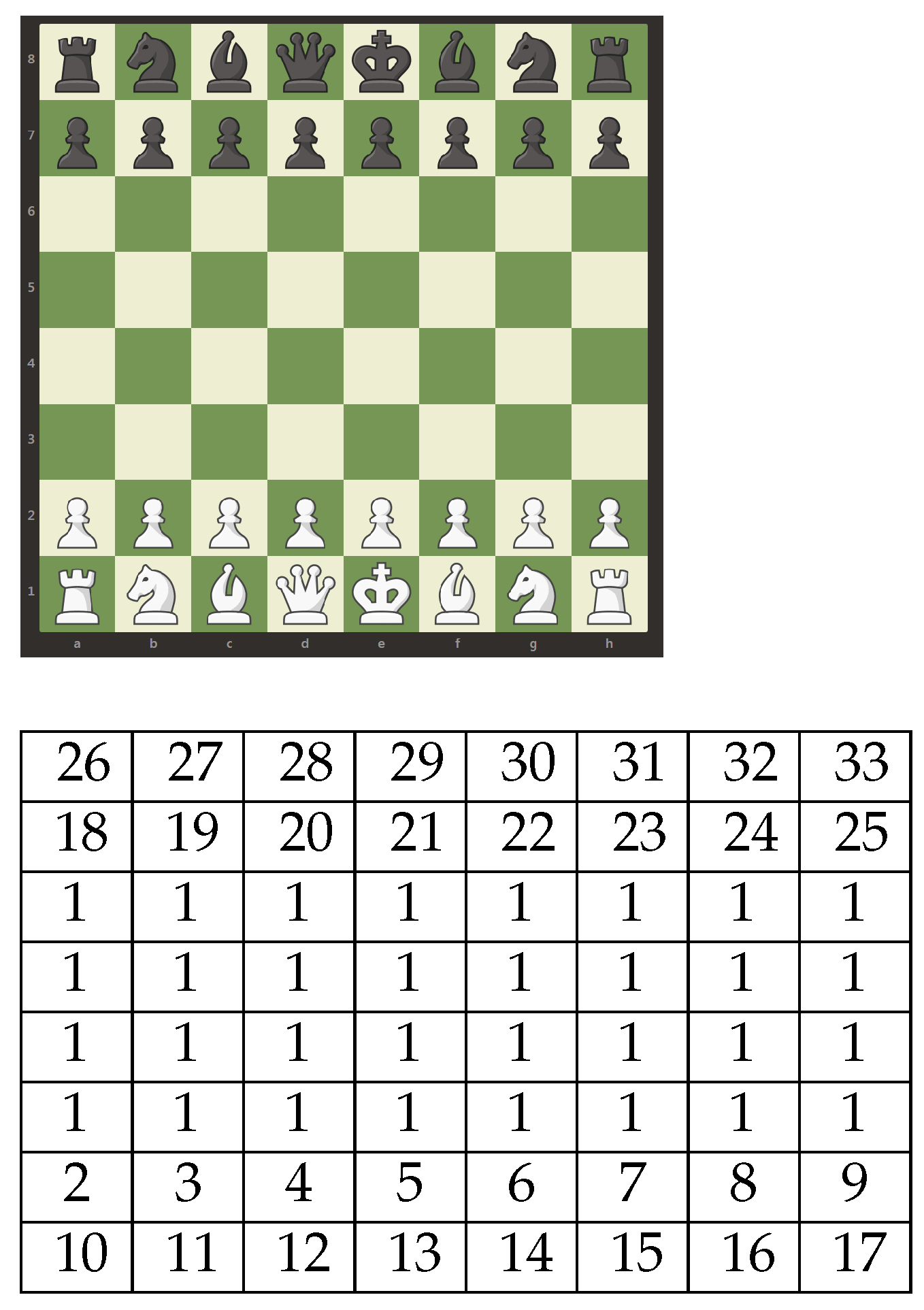
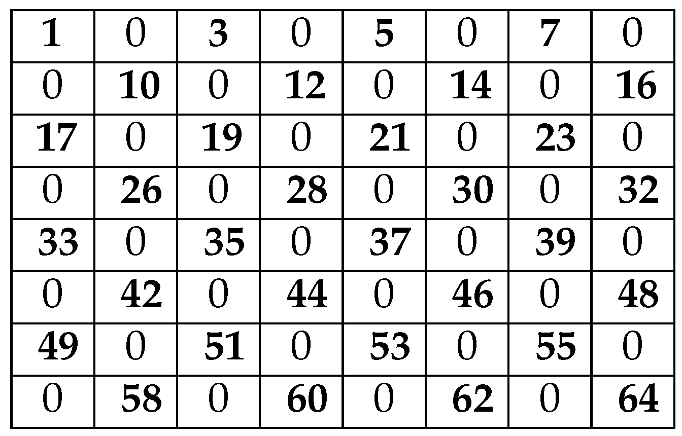
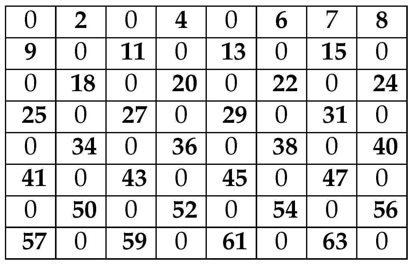
Figure 1 shows the starting board of any chess game. It consists of 64 cells where each of the two players (the white and the black), has 16 pieces. We encode this board as G-number b of 64 numbers, each of which encodes the contents of the corresponding cell. This number b can, when convenient for visualization, be construed as a matrix shown below the board picture in Figure 1.

An empty cell is encoded as 1. A white piece on the starting board is encoded as a number from 2 up to 17. Thus, west to east, the white pawns are encoded as 2, 3, 4, 5, 6, 7, 8, 9, the white rooks as 10 (west) and 17 (east), the white knights as 11 (west) and 16 (east), the white bishops as 12 (west or dark-colored) and 15 (east or light-colored), the white queen as 13, and the white king as 14.

A black piece on the starting board is encoded as a number from 18 up to 33. Thus, west to east, the black pawns are encoded as 18, 19, 20, 21, 22, 23, 24, 25, the black rooks as 26 (west) and 33 (east), the black knights as 27 (west) and 32 (east), the black bishops as 28 (west or light-colored) and 31 (east or dark-colored), the black queen as 29, and the black king as 30.

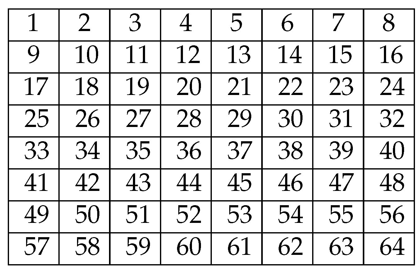
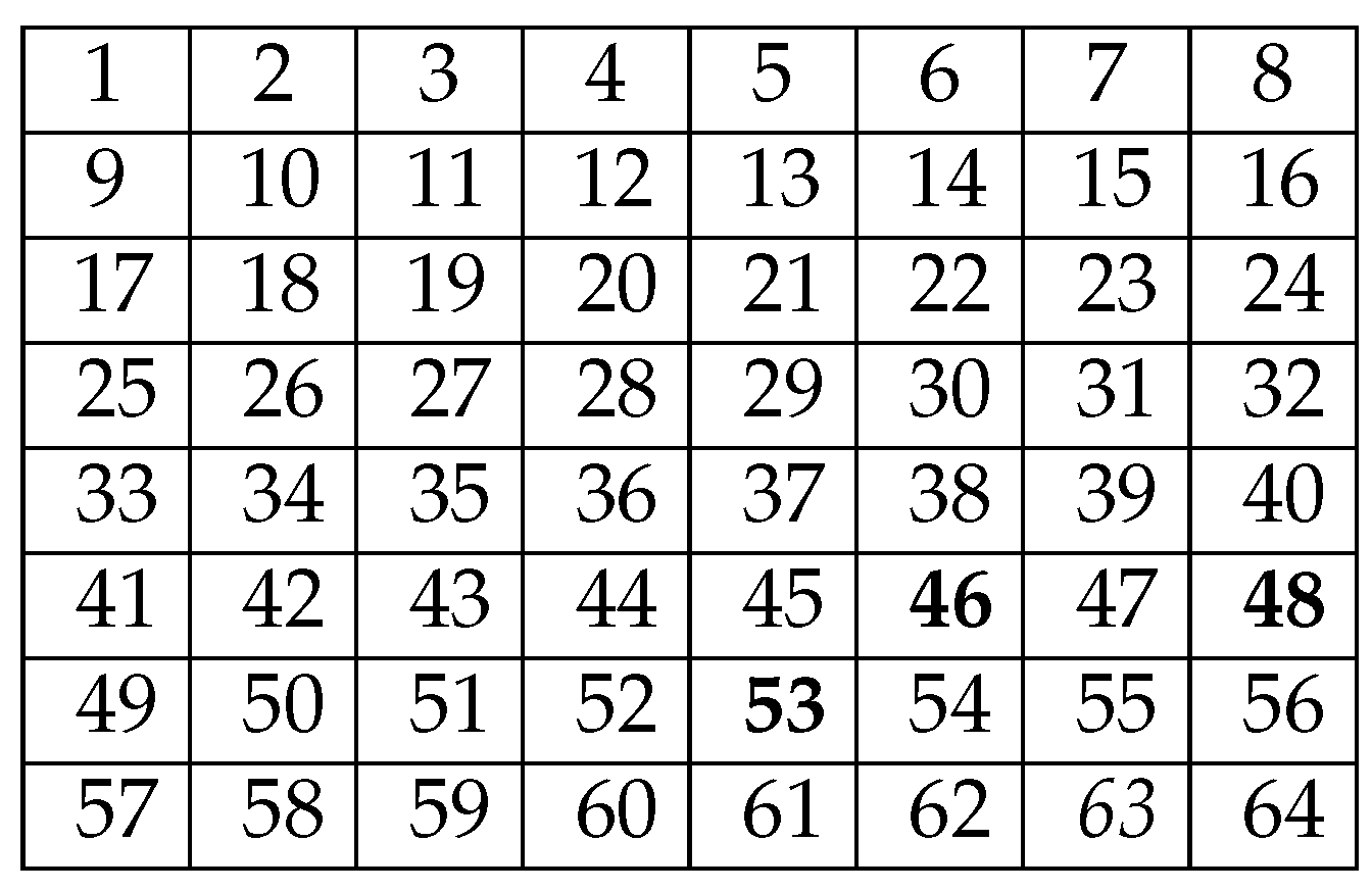
Each cell on board b has a unique position shown in Figure 2. Let

$$\begin{array}{ccc}{\zeta }_{ps}\hfill & =\hfill & \mathtt{g}\mathtt{g}\mathtt{n}(1,64,1)\hfill \end{array}$$

(32)

denote the G-number of all positions from 1 to 64. A position k is a valid position if $k\in {\zeta }_{ps}$. Thus, if b is the board in Figure 1, then

$$\begin{array}{ccc}{\left(b\right)}_1\hfill & =\hfill & 26;\hfill \\ {\left(b\right)}_2\hfill & =\hfill & 27;\hfill \\ {\left(b\right)}_{63}\hfill & =\hfill & 16;\hfill \\ {\left(b\right)}_{64}\hfill & =\hfill & 17;\hfill \\ {\left(b\right)}_i\hfill & =\hfill & 0,i<1\mathrm{or}i>64;\hfill \end{array}$$

and

$$(\forall i\in \mathtt{g}\mathtt{g}\mathtt{n}(17,48))\{{\left(b\right)}_i=1\}.$$

Since there are exactly 32 empty cells, we have

$$\mathtt{c}\mathtt{n}\mathtt{t}(1,b)=32.$$

The position of the black and white kings on any valid board b (valid boards are defined below) are

$$\begin{array}{ccc}& {\left(\mathtt{p}\mathtt{s}\mathtt{n}(14,b)\right)}_1;\hfill & \\ & {\left(\mathtt{p}\mathtt{s}\mathtt{n}(30,b)\right)}_1.\hfill & \end{array}$$

Thus, for b in Figure 1, we have

$$\begin{array}{ccc}& {\left(\mathtt{p}\mathtt{s}\mathtt{n}(14,b)\right)}_1=61;\hfill & \\ & {\left(\mathtt{p}\mathtt{s}\mathtt{n}(30,b)\right)}_1=5.\hfill & \end{array}$$

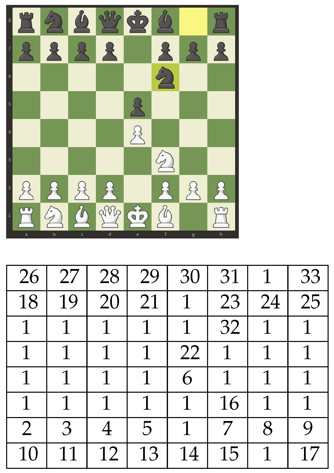
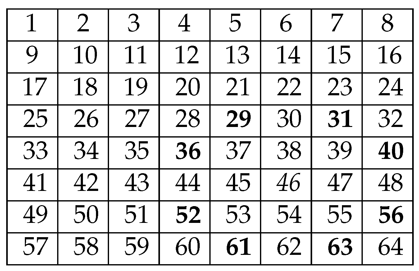
Figure 3 shows board $b^{\prime }$ that is the result of two moves made by each player on b in Figure 1. Thus, the following predicates are true:

$$\begin{array}{ccccccc}{\left(b\right)}_{53}=6\hfill & \wedge \hfill & {\left(b\right)}_{37}=1\hfill & \wedge \hfill & {\left(b^{\prime }\right)}_{53}=1\hfill & \wedge \hfill & {\left(b^{\prime }\right)}_{37}=6;\hfill \\ {\left(b\right)}_{63}=16\hfill & \wedge \hfill & {\left(b\right)}_{46}=1\hfill & \wedge \hfill & {\left(b^{\prime }\right)}_{63}=1\hfill & \wedge \hfill & {\left(b^{\prime }\right)}_{46}=16;\hfill \\ {\left(b\right)}_{13}=22\hfill & \wedge \hfill & {\left(b\right)}_{29}=1\hfill & \wedge \hfill & {\left(b^{\prime }\right)}_{13}=1\hfill & \wedge \hfill & {\left(b^{\prime }\right)}_{29}=22;\hfill \\ {\left(b\right)}_7=32\hfill & \wedge \hfill & {\left(b\right)}_{22}=1\hfill & \wedge \hfill & {\left(b^{\prime }\right)}_7=1\hfill & \wedge \hfill & {\left(b^{\prime }\right)}_{22}=32.\hfill \end{array}$$

4.2. Pawn Metamorphosis

If a pawn reaches the first row on the opposite side of the board, it transforms into a queen, a rook, a bishop, or a king of the same color. We call these positions metamorphic positions and give them in

Table 1. Metamorphic positions for the white and black pawns encoded as G-numbers and the symbols that denote the G-numbers.

Pawn	Metamorphic Positions
2	[1, 2, 3, 4, 5, 6, 7]
3	[1, 2, 3, 4, 5, 6, 7, 8]
4	[1, 2, 3, 4, 5, 6, 7, 8]
5	[1, 2, 3, 4, 5, 6, 7, 8]
6	[1, 2, 3, 4, 5, 6, 7, 8]
7	[1, 2, 3, 4, 5, 6, 7, 8]
8	[1, 2, 3, 4, 5, 6, 7, 8]
9	[2, 3, 4, 5, 6, 7, 8]
18	[57, 58, 59, 60, 61, 62, 63]
19	[57, 58, 59, 60, 61, 62, 63, 64]
20	[57, 58, 59, 60, 61, 62, 63, 64]
21	[57, 58, 59, 60, 61, 62, 63, 64]
22	[57, 58, 59, 60, 61, 62, 63, 64]
23	[57, 58, 59, 60, 61, 62, 63, 64]
24	[57, 58, 59, 60, 61, 62, 63, 64]
25	[58, 59, 60, 61, 62, 63, 64]

.

Let $2\le j\le 8$ be a white pawn and let k be one of its metamorphic positions. If j becomes a queen, the new white queen is encoded as $\langle \langle j,k\rangle ,37\rangle$; if j becomes a rook, the new white rook is encoded as $\langle \langle j,k\rangle ,41\rangle$; if j becomes a bishop, the new white bishop is encoded as $\langle \langle j,k\rangle ,43\rangle$; if j becomes a knight, the new white knight is encoded as $\langle \langle j,k\rangle ,47\rangle$.

Let $18\le j\le 25$ be a black pawn and let k be one of its metamorphic positions. If j becomes a queen, the new black queen is encoded as $\langle \langle j,k\rangle ,53\rangle$; if j becomes a rook, the new black rook is encoded as $\langle \langle j,k\rangle ,59\rangle$; if j becomes a bishop, the new black bishop is encoded as $\langle \langle j,k\rangle ,61\rangle$; if j becomes a knight, the new black knight is encoded as $\langle \langle j,k\rangle ,67\rangle$.

Thus, if white pawn 2 becomes a queen at position 7, the new white queen is $\langle \langle 2,7\rangle ,37\rangle$; if 2 becomes a rook at position 7, the new white rook is $\langle \langle 2,7\rangle ,41\rangle$; if 2 becomes a bishop at position 7, the new white bishop is $\langle \langle 2,7\rangle ,43\rangle$; if 2 becomes a knight, the new white knight is $\langle \langle 2,7\rangle ,47\rangle$.

Similarly, if black pawn 19 becomes a queen at position 59, the new black queen is $\langle \langle 19,59\rangle ,53\rangle$; if 19 becomes a rook at position 59, the new black rook is $\langle \langle 19,59\rangle ,59\rangle$; if 19 becomes a bishop at position 59, the new black bishop is $\langle \langle 19,59\rangle ,61\rangle$; if 19 becomes a knight at position 59, the new black knight is $\langle \langle 19,59\rangle ,67\rangle$.

Since for any z, $z=\langle x,y\rangle$, where x and y are unique (See Equation (5)), this encoding scheme for pawn metamorphosis ensures that every new piece is encoded as a unique number. Each player can obtain at most eight new pieces through pawn metamorphosis. The supplementary materials contain the encoding tables for all pieces that can be obtained through pawn metamorphosis.

We call the pieces into which the pawns transform at the metamorphic positions metamorphic pieces and refer to the pieces on the original board as regular pieces. Formally, j is a regular white piece if $j\in \mathtt{g}\mathtt{g}\mathtt{n}(2,17,1)$, is a regular black piece if $j\in \mathtt{g}\mathtt{g}\mathtt{n}(18,33,1)$, and is a regular piece if j is a regular white or black piece.

Tables S1 and S2 in the Supplementary Materials contain all unique numbers of the white and black pieces under this encoding scheme that can be obtained through pawn metamorphosis with the primitive recursive pairing function. Let

$$\begin{array}{ccc}\hfill & {\zeta }_{\mu }^w=[\langle \langle 2,1\rangle ,37\rangle ,\dots ,\langle \langle 9,8\rangle ,47\rangle ];\hfill & \\ \\ \hfill & {\zeta }_{\mu }^b=[\langle \langle 18,57\rangle ,53\rangle ,\dots ,\langle \langle 25,64\rangle ,67\rangle ]\hfill & \\ \end{array}$$

(33)

be the G-numbers of the white, black, and all metamorphic pieces.

4.3. Valid Pieces and Boards

Let the primitive recursive predicates

$$\begin{array}{ccc}\mathtt{w}\mathtt{p}\left(j\right)\hfill & \equiv \hfill & \{2\le j\le 17\}\vee \{j\in {\zeta }_{\mu }^w\};\hfill \\ \\ \mathtt{b}\mathtt{p}\left(j\right)\hfill & \equiv \hfill & \{18\le j\le 33\}\vee \{j\in {\zeta }_{\mu }^b\}\hfill \end{array}$$

(34)

hold when j is a valid white or black piece, respectively. A chess piece j is valid if and only if the primitive recursive predicate

$$\mathtt{v}\mathtt{l}\mathtt{p}\left(j\right)\equiv \mathtt{w}\mathtt{p}\left(j\right)\vee \mathtt{b}\mathtt{p}\left(j\right).$$

holds (i.e., $\mathtt{v}\mathtt{l}\mathtt{p}\left(j\right)=1$). Let

$$\begin{array}{ccc}{\zeta }_{wp}\hfill & =\hfill & \mathtt{g}\mathtt{g}\mathtt{n}(2,17,1){\otimes }_r{\zeta }_{\mu }^w;\hfill \\ {\zeta }_{bp}\hfill & =\hfill & \mathtt{g}\mathtt{g}\mathtt{n}(18,33,1){\otimes }_r{\zeta }_{\mu }^b;\hfill \\ {\zeta }_{cp}\hfill & =\hfill & {\zeta }_{wp}{\otimes }_r{\zeta }_{bp}\hfill \end{array}$$

(35)

denote the G-numbers of the white pieces (${\zeta }_{wp}$), the black pieces (${\zeta }_{bp}$), and all chess pieces (${\zeta }_{cp}$).

Let us consider if the valid chess board characteristic is pr-decidable. If b is a valid chess board, it must contain exactly one white king (14) and exactly one black king (30). The primitive recursive predicate

$$P_1\left(b\right)\equiv \mathtt{c}\mathtt{n}\mathtt{t}(14,b)=\mathtt{c}\mathtt{n}\mathtt{t}(30,b)=1$$

holds when b has this characteristic.

Board b is valid if the number of occurrences of each regular or metamorphic piece on b, with the exception of the two kings, is 0 (if the piece is captured) or exactly 1 (if the piece is not captured). The primitive recursive predicate

$$\begin{array}{ccccc}{P}_2\left(b\right)\hfill & \equiv \hfill & (\forall i\in {\zeta }_{cp})\{\{i=14\vee i=30\}\vee \mathtt{c}\mathtt{n}\mathtt{t}(i,b)\le 1\}\hfill & & \end{array}$$

ensures that the number of occurrences for each piece on b, regular or metamorphic, so long as that piece is not a king, is 0 or 1.

If b is valid, then the count of the empty cells on it is at least 32 (i.e., b is the starting board) and at most 62 (i.e., when only the kings are present). The primitive recursive predicate

$$\begin{array}{ccccc}{P}_3\left(b\right)\hfill & \equiv \hfill & 32\le \mathtt{c}\mathtt{n}\mathtt{t}(1,b)\le 62\hfill & & \end{array}$$

holds when the count of the empty cells on b is between 32 and 62.

If board b is valid, then the regular and metamorphic black and white bishops, when present on b, must be in the appropriate light-colored and dark-colored positions. Tables S3–S6 in the Supplementary Materials contain the encoding tables for all metamorphic light-colored and dark-colored bishops.

Let ${\zeta }_{\mu }^{lc,wb}$ denote the G-number of the numbers of the metamorphic light-colored white bishops in Table S3, ${\zeta }_{\mu }^{dc,wb}$—the G-number of the numbers of the metamorphic dark-colored white bishops in Table S4, ${\zeta }_{\mu }^{lc,bb}$—the G-number of the numbers of the metamorphic light-colored black bishops in Table S5, ${\zeta }_{\mu }^{dc,bb}$—the G-number of the numbers of the metamorphic dark-colored black bishops in Table S6. Let

$$\begin{array}{ccc}{\zeta }_{\mu }^{lcb}\hfill & =\hfill & {\zeta }_{\mu }^{lc,wb}{\oplus }_r{\zeta }_{\mu }^{lc,bb};\hfill \\ \\ {\zeta }_{\mu }^{dcb}\hfill & =\hfill & {\zeta }_{\mu }^{dc,wb}{\oplus }_r{\zeta }_{\mu }^{dc,bb}\hfill \end{array}$$

(36)

be the G-numbers of the light-colored and dark-colored metamorphic bishops.

The primitive recursive predicates

$$\begin{array}{ccc}{\mathtt{w}\mathtt{k}}_{\mu }\left(j\right)\hfill & \equiv \hfill & j\in {\zeta }_{\mu }^w\wedge r\left(j\right)=47;\hfill \\ \\ {\mathtt{b}\mathtt{k}}_{\mu }\left(j\right)\hfill & \equiv \hfill & j\in {\zeta }_{\mu }^b\wedge r\left(j\right)=67\hfill \end{array}$$

(37)

hold if j is a metamorphic white or black knight, respectively. The primitive recursive predicates

$$\begin{array}{ccc}{\mathtt{w}\mathtt{l}\mathtt{b}}_{\mu }\left(j\right)\hfill & \equiv \hfill & j\in {\zeta }_{\mu }^{lcb}\wedge r\left(j\right)=43;\hfill \\ \\ {\mathtt{b}\mathtt{l}\mathtt{b}}_{\mu }\left(j\right)\hfill & \equiv \hfill & j\in {\zeta }_{\mu }^{lcb}\wedge r\left(j\right)=61\hfill \end{array}$$

(38)

hold if j is a metamorphic white or black light-colored bishop, respectively. The primitive recursive predicates

$$\begin{array}{ccc}{\mathtt{w}\mathtt{d}\mathtt{b}}_{\mu }\left(j\right)\hfill & \equiv \hfill & j\in {\zeta }_{\mu }^{dcb}\wedge r\left(j\right)=43;\hfill \\ \\ {\mathtt{b}\mathtt{d}\mathtt{b}}_{\mu }\left(j\right)\hfill & \equiv \hfill & j\in {\zeta }_{\mu }^{dcb}\wedge r\left(j\right)=61;\hfill \end{array}$$

(39)

hold if j is a metamorphic white or black dark-colored knight, respectively. The primitive recursive predicates

$$\begin{array}{ccc}{\mathtt{k}\mathtt{n}}_{\mu }\left(j\right)\hfill & \equiv \hfill & {\mathtt{w}\mathtt{k}}_{\mu }\left(j\right)\vee {\mathtt{b}\mathtt{k}}_{\mu }\left(j\right);\hfill \\ \\ {\mathtt{b}\mathtt{h}}_{\mu }\left(j\right)\hfill & \equiv \hfill & {\mathtt{w}\mathtt{d}\mathtt{b}}_{\mu }\left(j\right)\vee {\mathtt{b}\mathtt{d}\mathtt{b}}_{\mu }\left(j\right)\hfill \end{array}$$

(40)

hold if j is a metamorphic knight or bishop, respectively.

If board b is valid, then the regular light-colored bishops 15 and 28 and any metamorphic light-colored bishops, when present, must be located on the light-colored positions and the regular dark-color bishops 12 and 31 and any metamorphic dark-colored bishops, when present, must be located on the dark-colored positions. Let

$$\begin{array}{c}{\zeta }_{lps}=[1,3,5,7,10,12,14,16,17,19,21,23,26,28,30,32,33,\hfill \\ 35,37,39,42,44,46,48,49,51,53,55,58,60,62,64]\hfill \end{array}$$

(41)

be the G-number of all light-colored positions on b (See Figure 4) and let

$$\begin{array}{c}{\zeta }_{dps}=[2,4,6,8,9,11,13,15,18,20,22,24,25,27,29,31,34,\hfill \\ 36,38,40,41,43,45,47,50,52,54,56,57,59,61,63]\hfill \end{array}$$

(42)

be the G-number of all dark-colored positions on b (See Figure 5). The primitive recursive predicate

$$\begin{array}{ccccc}{P}_4\left(b\right)\hfill & \equiv \hfill & \{(\forall j\in [15,28]{\oplus }_r{\zeta }_{\mu }^{lcb})\{j\notin b\vee {\left(\mathtt{p}\mathtt{s}\mathtt{n}(j,b)\right)}_1\in {\zeta }_{lps}\}\wedge \hfill & & \\ & & \{(\forall j\in [12,31]{\oplus }_r{\zeta }_{\mu }^{dcb})\{j\notin b\vee {\left(\mathtt{p}\mathtt{s}\mathtt{n}(j,b)\right)}_1\in {\zeta }_{dps}\}\hfill & & \end{array}$$

holds of b when all bishops, if present, are in the positions of the appropriate color.

If b is valid, then the regular white pawns 2–9 or the regular black pawns 18–25 cannot be in the metamorphic positions 1–8 and 57–64 (See Figure 1 and Figure 2). Let

$$\begin{array}{ccc}{\rho }_{\mu }\hfill & =\hfill & \mathtt{g}\mathtt{g}\mathtt{n}(1,8,1){\otimes }_r\mathtt{g}\mathtt{g}\mathtt{n}(57,64,1)\hfill \end{array}$$

be the G-number of positions 1–8 and 57–64. The primitive recursive predicate

$$\begin{array}{cc}{P}_5\left(b\right)\equiv \hfill & \{(\forall j\in \mathtt{g}\mathtt{g}\mathtt{n}(2,9,1))\{j\notin b\vee {\left(\mathtt{p}\mathtt{s}\mathtt{n}(j,b)\right)}_1\notin {\rho }_{\mu }\}\wedge \hfill \\ \hfill & \left\{(\forall j\in \mathtt{g}\mathtt{g}\mathtt{n}(18,25,1))\{j\notin b\vee {\left(\mathtt{p}\mathtt{s}\mathtt{n}(j,b)\right)}_1\notin {\rho }_{\mu }\}\right\}\hfill \end{array}$$

holds of b when the regular white and black pawns do not occupy the positions they cannot occupy either because they cannot move backward to reach those positions or because they undergo metamorphosis on those positions. In summary, the primitive recursive predicate

$$\mathtt{v}\mathtt{l}\mathtt{d}\left(b\right)\equiv \mathtt{L}\mathtt{t}\left(b\right)=64\wedge P_1\left(b\right)\wedge P_2\left(b\right)\wedge P_3\left(b\right)\wedge P_4\left(b\right)\wedge P_5\left(b\right)$$

(43)

holds if b is a valid 64-cell chess board. Thus, if $b_1$ and $b_2$ are the boards in Figure 1 and Figure 3, respectively, then $\mathtt{v}\mathtt{l}\mathtt{d}\left(b_1\right)=\mathtt{v}\mathtt{l}\mathtt{d}\left(b_2\right)=1$.

4.4. Diagonals, Rows, Columns

A position $1\le k\le 64$ on valid b is a member of at most two diagonals. Let $k^{\prime }\in \{1,2\}$ and $d_{k,k^{\prime }}$ be the diagonals (if $k^{\prime }=2$) or the diagonal that include k. For example, $k=62$ is a member of two diagonals: $d_{62,1}=[48,55,62]$ and $d_{62,2}=[17,26,35,44,53,62]$ (See Figure 2); and $k=1$ is a member of the diagonal $d_{1,1}=[1,10,19,28,37,46,55,64]$ (i.e., the first main diagonal).

Let

$$D=[\langle 1,\left[d_{1,1}\right]\rangle ,\langle 2,[d_{2,1},d_{2,2}]\rangle ,\langle 3,[d_{3,1},d_{3,2}],\rangle ,\dots ,\langle 64,\left[d_{64,1}\right]\rangle ]$$

be the G-number that pairs each position k with the diagonals that contain it.

Since each position is a member of exactly one row and exactly one column, we define G-numbers R and C to pack all rows and columns. For example, 7 is in the row $[1,2,3,4,5,6,7,8]$ and the column $[7,15,23,31,39,47,55,63]$.

Let

$$\begin{array}{ccc}{F}_8\left(0\right)\hfill & =\hfill & 1\hfill \\ F_8(t+1)\hfill & =\hfill & F_8\left(t\right)+8\hfill \end{array}$$

and

$$F_9\left(r\right)=\left\{\begin{array}{cc}\mathtt{g}\mathtt{g}\mathtt{n}(F_8(r\dot{-}1),F_8(r\dot{-}1)+7,1)\hfill & \mathrm{if}1\le r\le 8,\hfill \\ 0\hfill & \mathrm{otherwise}.\hfill \end{array}\right.$$

Since $F_8(·)$ is primitive recursive by definition, $F_9(·)$ is primitive recursive by the DCT. Thus,

$$\begin{array}{ccc}{F}_9\left(1\right)\hfill & =\hfill & \mathtt{g}\mathtt{g}\mathtt{n}(F_8\left(0\right),F_8\left(0\right)+7,1)=\prod _{j=1}^8\pi {\left(j\right)}^j;\hfill \\ \\ F_9\left(2\right)\hfill & =\hfill & \mathtt{g}\mathtt{g}\mathtt{n}(F_8\left(1\right),F_8\left(1\right)+7,1)=\prod _{j=9}^{16}\pi {\left(j\right)}^j;\hfill \\ \\ F_9\left(8\right)\hfill & =\hfill & \mathtt{g}\mathtt{g}\mathtt{n}(F_8\left(7\right),F_8\left(7\right)+7,1)=\prod _{j=57}^{64}\pi {\left(j\right)}^j.\hfill \end{array}$$

We place all row numbers on valid b into G-number R to pair each row number with the G-number of all positions in that row:

$$\begin{array}{ccc}R\hfill & =\hfill & \prod _{r=1}^8\langle r,F_9\left(r\right)\rangle .\hfill \end{array}$$

For each $1\le i\le 8$, we define eight primitive recursive functions (one for each column)

$$\begin{array}{ccc}{\kappa }_i\left(0\right)\hfill & =\hfill & i,\hfill \\ {\kappa }_i(t+1)\hfill & =\hfill & {\kappa }_i\left(t\right)+8\hfill \end{array}$$

and let

$$c_i=\prod _{j={\kappa }_i\left(0\right)}^{{\kappa }_i\left(7\right)}\pi {\left(j\right)}^j.$$

We place all column numbers into the G-number C that pairs each column number with the G-number of all positions in the column:

$$\begin{array}{ccc}C\hfill & =\hfill & \prod _{i=1}^8\langle i,c_i\rangle .\hfill \end{array}$$

The primitive recursive functions in (44)–(46) return the G-number of the diagonals, rows, and columns, respectively, for a valid position k on b.

$$\mathtt{d}\mathtt{g}\mathtt{s}\left(k\right)=r\left({\left(D\right)}_{\mathtt{a}\mathtt{s}\mathtt{c}(k,D)}\right)$$

(44)

$$\mathtt{r}\mathtt{w}\mathtt{s}\left(k\right)=r\left({\left(R\right)}_{\mathtt{a}\mathtt{s}\mathtt{c}(k,R)}\right)$$

(45)

$$\mathtt{c}\mathtt{l}\mathtt{s}\left(k\right)=r\left({\left(C\right)}_{\mathtt{a}\mathtt{s}\mathtt{c}(k,C)}\right)$$

(46)

Thus,

$$\begin{array}{ccccc}\mathtt{d}\mathtt{g}\mathtt{s}\left(62\right)\hfill & =\hfill & [d_{62,1},d_{62,2}]\hfill & & \\ & =\hfill & \left[\right[48,55,62],[17,26,35,44,53,62\left]\right];\hfill & & \\ {\left(\mathtt{d}\mathtt{g}\mathtt{s}\left(62\right)\right)}_1\hfill & =\hfill & d_{62,1};\hfill & & \\ {\left(\mathtt{d}\mathtt{g}\mathtt{s}\left(62\right)\right)}_2\hfill & =\hfill & d_{62,2};\hfill & & \\ \mathtt{r}\mathtt{w}\mathtt{s}\left(62\right)\hfill & =\hfill & [57,58,59,60,61,62,63,64];\hfill & & \\ \mathtt{c}\mathtt{l}\mathtt{s}\left(62\right)\hfill & =\hfill & [6,14,22,30,38,46,54,62].\hfill & & \end{array}$$

Given positions $k_1$ and $k_2$, let

$$z_d=\mathtt{d}\mathtt{g}\mathtt{s}\left(k_1\right){\otimes }_r\mathtt{d}\mathtt{g}\mathtt{s}\left(k_2\right)$$

and

$$F_{10}(k_1,k_2)={\displaystyle \underset{t\le Lt\left(z_d\right)}{\min }}\{k_1\in {\left(z_d\right)}_t\wedge k_2\in {\left(z_d\right)}_t\}.$$

  The primitive recursive function $\mathtt{d}\mathtt{g}(k_1,k_2)$ returns diagonal d that contains both $k_1$ and $k_2$ if d exists.

$$\mathtt{d}\mathtt{g}(k_1,k_2)={\left(z_d\right)}_{F_{10}(k_1,k_2)}$$

(47)

Let $z_r=\left[\mathtt{r}\mathtt{w}\mathtt{s}\left(k_1\right)\right]{\otimes }_r[\mathtt{r}\mathtt{w}\mathtt{s}\left(k_2\right)$] and

$$F_{11}(k_1,k_2)={\displaystyle \underset{t\le Lt\left(z_r\right)}{\min }}\{k_1\in {\left(z_r\right)}_t\wedge k_2\in {\left(z_r\right)}_t\}.$$

  The primitive recursive function $\mathtt{r}\mathtt{w}(k_1,k_2)$ returns row r that contains both $k_1$ and $k_2$ if r exists.

$$\mathtt{r}\mathtt{w}(k_1,k_2)={\left(z_r\right)}_{F_{11}(k_1,k_2)}$$

(48)

Let $z_c=\left[\mathtt{c}\mathtt{l}\mathtt{s}\left(k_1\right)\right]{\otimes }_r[\mathtt{c}\mathtt{l}\mathtt{s}\left(k_2\right)$] and

$$F_{12}(k_1,k_2)={\displaystyle \underset{t\le Lt\left(z_c\right)}{\min }}\{k_1\in {\left(z_c\right)}_t\wedge k_2\in {\left(z_c\right)}_t\}.$$

  The primitive recursive function $\mathtt{c}\mathtt{l}(k_1,k_2)$ returns column c that contains both $k_1$ and $k_2$ if c exists.

$$\mathtt{c}\mathtt{l}(k_1,k_2)={\left(z_c\right)}_{F_{12}(k_1,k_2)}$$

(49)

4.5. Potentially Reachable Positions

The primitive recursive predicate

$$\mathtt{o}\mathtt{c}(x,y)\equiv \left\{\mathtt{w}\mathtt{p}\right(x)\wedge \mathtt{b}\mathtt{p}(y\left)\right\}\vee \left\{\mathtt{w}\mathtt{p}\right(y)\wedge \mathtt{b}\mathtt{p}(x\left)\right\}$$

(50)

holds for valid pieces x and y of the opposite colors.

Let j, k, and b denote a valid piece, a valid position, and a valid board, respectively. Position $k^{\prime }\ne k$ on b is potentially reachable for j from k if j can move from k to $k^{\prime }$ on b. Position $k^{\prime }$ can be empty or occupied by a different piece.

Let $L_j^k$ be the G-number of the positions potentially reachable by j from k on b. For example, $L_{15}^1$ is the G-number of the positions potentially reachable by bishop 15 from position 1. The G-numbers $L_{15}^k$, $k\in [10,19,28,37,46,55,64]$, denote the positions potentially reachable by 15 from the other positions of the first main diagonal. We note that $L_j^k$ is defined regardless of any b in the sense that whether $k^{\prime }$ is potentially reachable for j from k depends only on the move rules for j and not on the positions of the other pieces on b.

Thus, for bishop 15 positioned anywhere on the first main diagonal, we have

$$\begin{array}{c}{L}_{15}^1=\langle 1,[10,19,28,37,46,55,64]\rangle ;\hfill \\ L_{15}^{10}=\langle 10,[1,3,17,19,28,37,46,55,64]\rangle ;\hfill \\ L_{15}^{19}=\langle 19,[1,10,5,12,26,33,28,37,46,55,64]\rangle ;\hfill \\ L_{15}^{28}=\langle 28,[1,10,19,7,14,21,35,42,49,37,46,55,64]\rangle ;\hfill \\ L_{15}^{37}=\langle 37,[1,10,19,28,16,23,30,44,51,58,46,55,64]\rangle ;\hfill \\ L_{15}^{46}=\langle 46,[1,10,19,28,37,32,39,53,60,55,64]\rangle ;\hfill \\ L_{15}^{55}=\langle 55,[1,10,19,28,37,46,48,62,64]\rangle ;\hfill \\ L_{15}^{64}=\langle 64,[1,10,19,28,37,46,55]\rangle .\hfill \end{array}$$

We recall that ${\zeta }_{lps}$ in (41) is the G-number of the light-colored positions on b. Since 15 is light-colored, the G-number

$$L_{15}={\otimes }_r{|}_{k\in {\zeta }_{lps}}\left[L_{15}^k\right]$$

contains all positions potentially reachable by 15. We observe that if j is another real or metamorphic light-colored black bishop (e.g., $j=28$), then

$$L_j=L_{15}.$$

For the dark-colored real bishops 12 and 31 (or any dark-colored metamorphic bishop j), we can analogously define $L_{12}=L_{31}=L_j$ using ${\zeta }_d$ in (42) (i.e., the G-number of the dark-colored positions on valid b).

In general, for each valid piece j we define the G-number of all potentially reachable positions on b and place all such G-numbers into L in (51) of the pairs $\langle j,L_j\rangle$, where $L_j$ is the G-number of all reachable positions for j on b.

$$L=\left({\otimes }_r{|}_{j=2}^{33}\left[\langle j,L_j\rangle \right]\right){\otimes }_r\left({\otimes }_r{|}_{j\in {\zeta }_{\mu }^w{\otimes }_r{\zeta }_{\mu }^b}\left[\langle j,L_j\rangle \right]\right)$$

(51)

The function

$$\mathtt{r}\mathtt{p}(j,k,b)=\left\{\begin{array}{cc}r\left(\mathtt{a}\mathtt{s}\mathtt{c}\right(k,r\left(\mathtt{a}\mathtt{s}\mathtt{c}\right(j,L\left)\right)\left)\right)\hfill & \mathrm{if}\mathtt{v}\mathtt{l}\mathtt{p}\left(j\right)\wedge \mathtt{v}\mathtt{l}\mathtt{d}\left(b\right)\hfill \\ 0\hfill & \mathrm{otherwise}\hfill \end{array}\right.$$

(52)

returns the G-number of all potentially reachable positions for j from k on b. The function $\mathtt{r}\mathtt{p}(·)$ is primitive recursive by the DCT.

Thus, if b and $b^{\prime }$ are boards in Figure 1 and Figure 3, respectively, then (See Figure 6 and Figure 7)

$$\begin{array}{ccc}\mathtt{r}\mathtt{p}(16,63,b)\hfill & =\hfill & [53,46,48];\hfill \\ \\ \mathtt{r}\mathtt{p}(16,46,b^{\prime })\hfill & =\hfill & [61,52,36,29,31,40,56,63].\hfill \end{array}$$

4.6. Actual Reachability for Bishop 15

If $k^{\prime }\in \mathtt{r}\mathtt{p}(j,k,b)$, it may be occupied by $j^{\prime }\ne j$ of the same color. For example, although $52\in \mathtt{r}\mathtt{p}(16,46,b^{\prime })$, ${\left(b^{\prime }\right)}_{52}=5\ne 1$, i.e., it is occupied by pawn 5 of the same color as knight 16 and, consequently, 16 cannot move from 46 to 52 on $b^{\prime }$. To put it differently, 52 is not actually reachable for 16 from 46 on $b^{\prime }$.

The characteristics of potential reachability and actual reachability, while conceptually related by the rules of chess, are different in that the potential reachability of $k^{\prime }$ for j from k holds on any valid b whereas the actual reachability of $k^{\prime }$ for j from k depends not only on whether $k^{\prime }\in \mathtt{r}\mathtt{p}(j,k,b)$ but also on ${\left(b\right)}_{k^{\prime }}$.

As an extended example, let us consider the characteristic of actual reachability for bishop 15 to determine if this characteristic is pr-computable. For any valid position k of 15 on b, the positions in the G-number of actually reachable positions for 15 from k depend on the light-colored bishop move rules and require us to take into account the positions of the other pieces of the same color on b.

Let the primitive recursive function

$$\mathtt{c}\mathtt{p}\mathtt{s}\mathtt{n}(j,b)=\left\{\begin{array}{cc}{\left(\mathtt{p}\mathtt{s}\mathtt{n}(j,b)\right)}_1\hfill & \mathrm{if}\mathtt{v}\mathtt{l}\mathtt{p}\left(j\right)\wedge \mathtt{v}\mathtt{l}\mathtt{d}\left(b\right),\hfill \\ 0\hfill & \mathrm{otherwise}\hfill \end{array}\right.$$

(53)

return the current position of valid piece j on valid board b so that if $j\in b$, then

$${\left(b\right)}_{\mathtt{c}\mathtt{p}\mathtt{s}\mathtt{n}(j,b)}=j.$$

Let $\mathtt{c}\mathtt{p}\mathtt{s}\mathtt{n}(15,b)=k_{15}$. We seek to compute the G-number of actually reachable positions for 15 from $k_{15}$ on b. Let $k\ne k_{15}$ be a valid position. Then $\mathtt{d}\mathtt{g}(k_{15},k)$ in (49) returns diagonal d that contains both $k_{15}$ and k. If d does not exist (i.e., $d=0$), then k is not actually reachable for 15 from $k_{15}$ on b. If d exists, we need to ensure that either k is empty on b (i.e., ${\left(b\right)}_k=1$) or is occupied by a piece of the opposite color $\mathtt{o}\mathtt{c}({\left(b\right)}_k,15)=1$ and 15 can capture ${\left(b\right)}_k$. Furthermore, if d exists, we need to ensure that there is no piece either of the same or opposite color between $k_{15}$ and k on d. The primitive recursive predicate

$$\begin{array}{ccc}{P}_6(k,k_{15},b)\hfill & \equiv \hfill & \mathtt{v}\mathtt{l}\mathtt{d}\left(b\right)\hfill \\ \hfill & \wedge \hfill & k\ne k_{15}\hfill \\ \hfill & \wedge \hfill & k\in \mathtt{r}\mathtt{p}(15,k_{15},b)\hfill \\ \hfill & \wedge \hfill & \mathtt{d}\mathtt{g}(k_{15},k)\ne 0\hfill \\ \hfill & \wedge \hfill & (\forall k^{\prime }\in \mathtt{d}\mathtt{g}(k_{15},k))\{\hfill \\ \hfill & \hfill & \{k^{\prime }=k\vee k^{\prime }=k_{15}\}\vee {\left(b\right)}_{k^{\prime }}=1\}\hfill \\ \hfill & \wedge \hfill & \{{\left(b\right)}_k=1\vee \mathtt{o}\mathtt{c}(15,{\left(b\right)}_k)\}\hfill \end{array}$$

holds on b if k is potentially reachable for 15 from $k_{15}$ and is on the same diagonal with $k_{15}$ and every position $k^{\prime }$ between k and $k_{15}$ on the diagonal is empty and k itself is either empty or occupied by a black piece. The primitive recursive predicate

$${\mathtt{a}\mathtt{r}\mathtt{p}}_{15}(k,k_{15},b)\equiv P_6(k,k_{15},b)$$

holds when k is actually reachable for 15 from $k_{15}$ on valid b.

Let $b^{\prime }$ be the board in Figure 3. Then

$${\mathtt{a}\mathtt{r}\mathtt{p}}_{15}(48,62,b^{\prime })=0,$$

because $\mathtt{d}\mathtt{g}(62,48)=d_{62,1}=[48,55,62]$, but pawn 8 in position 55 is of the same color with 15, which makes $P_6(48,62,b^{\prime })$ false. On the other hand,

$${\mathtt{a}\mathtt{r}\mathtt{p}}_{15}(k,62,b^{\prime })=1,$$

for any $k\in \{17,26,35,44,53\}$. Let b be a board and let

$${\mathtt{a}\mathtt{r}\mathtt{p}}_{15}^{\prime }\left(k\right)\equiv {\mathtt{a}\mathtt{r}\mathtt{p}}_{15}(k,k_{15},b).$$

Then for any $k_{15}$ on b,

$${\mathtt{m}\mathtt{a}\mathtt{p}}_{{\mathtt{a}\mathtt{r}\mathtt{p}}_{15}^{\prime }\left(k\right)}\left({\zeta }_{lps}\right)$$

computes in a primitive recursive fashion the G-number of all positions actually reachable for 15 from $k_{15}$ on b (See Equation (41) for ${\zeta }_{lps}$), which furnishes us the following lemma.

Lemma 1.

Actual reachability for bishop 15 is pr-decidable and pr-computable.

4.7. Actual Reachability

Let j be a valid piece on valid b. Let $j={\left(b\right)}_{k_j}$, where

$$k_j=\mathtt{c}\mathtt{p}\mathtt{s}\mathtt{n}(j,b)$$

(54)

is the pr-computable position of j on b. Thus, $k_{30}$ is the position of the black king on b and $k_{14}$ is the position of the white king on b.

Let $k\in \mathtt{r}\mathtt{p}(j,k_j,b)$. By the rules of chess, j can actually reach finitely many positions from $k_j$. Consequently, whether k is actually reachable for j from $k_j$ on b can be decided in a primitive recursive fashion with the functions and predicates in Section 2 and Section 3 and $\mathtt{o}\mathtt{c}(·)$, $\mathtt{v}\mathtt{l}\mathtt{d}(·)$, $\mathtt{d}\mathtt{g}(·)$, $\mathtt{r}\mathtt{w}(·)$, $\mathtt{c}\mathtt{l}(·)$, $\mathtt{p}\mathtt{s}\mathtt{n}(·)$, $\mathtt{r}\mathtt{p}(\dot{)}$ through appropriate Boolean combinations of primitive recursive predicates and applications of the DCT in the way similar to the one constructed for bishop 15 in the previous section. Hence, we have the following lemma.

Lemma 2.

Let $\mathtt{v}\mathtt{l}\mathtt{p}\left(j\right)=\mathtt{v}\mathtt{l}\mathtt{d}\left(b\right)=1$ and $k\in \mathtt{r}\mathtt{p}(j,k_j,b)$. Then ${\mathtt{a}\mathtt{r}\mathtt{p}}_j(k,k_j,b)$ is primitive recursive.

Since there are finitely many regular and metamorphic pieces, there are finitely many predicates ${\mathtt{a}\mathtt{r}\mathtt{p}}_j(·)$. Let $z=\mathtt{r}\mathtt{p}(j,k_j,b)$. The function

$$\begin{array}{ccc}\mathtt{a}\mathtt{r}\mathtt{x}(z,j,k_j,b,0)\hfill & =\hfill & \left[\right],\hfill \\ \mathtt{a}\mathtt{r}\mathtt{x}(z,j,k_j,b,t+1)\hfill & =\hfill & F_{13}(z,j,k_j,b,\hfill \\ \hfill & \hfill & \mathtt{a}\mathtt{r}\mathtt{x}(z,j,k_j,b,t),\hfill \\ \hfill & \hfill & s\left(t\right)),\hfill \end{array}$$

where

$$F_{13}(z,j,k_j,b,y,i)=\left\{\begin{array}{cc}y\hfill & \mathrm{if}{\left(z\right)}_i\notin {\mathtt{a}\mathtt{r}\mathtt{p}}_j(j,k_j,b),\hfill \\ \left[{\left(z\right)}_i\right]{\otimes }_{l}y\hfill & \mathrm{if}{\left(z\right)}_i\in {\mathtt{a}\mathtt{r}\mathtt{p}}_j(j,k_j,b)\hfill \end{array}\right.$$

returns the G-number of all positions in z that are actually reachable for j from $k_j$ on b. The function $F_{13}(·)$ is primitive recursive by Lemma 1 and the DCT, which makes $\mathtt{a}\mathtt{r}\mathtt{x}(·)$ also primitive recursive.

The function $\mathtt{a}\mathtt{r}\mathtt{p}\mathtt{s}(·)$ in (55) returns the G-number of actually reachable positions for j from $k_j$ on b. This function is primitive recursive, because it is composed from primitive recursive functions.

$$\begin{array}{c}\mathtt{a}\mathtt{r}\mathtt{p}\mathtt{s}(j,k_j,b)=\mathtt{a}\mathtt{r}\mathtt{x}(\mathtt{r}\mathtt{p}(j,k_j,b),j,k_j,b,\mathtt{L}\mathtt{t}\left(\mathtt{r}\mathtt{p}(j,k_j,b)\right))\hfill \end{array}$$

(55)

Thus, if b and $b^{\prime }$ are the boards in Figure 1 and Figure 3, respectively, then

$$\begin{array}{c}\mathtt{a}\mathtt{r}\mathtt{p}\mathtt{s}(15,62,b)=\left[\right];\hfill \\ \mathtt{a}\mathtt{r}\mathtt{p}\mathtt{s}(16,63,b)=[46,48];\hfill \\ \mathtt{a}\mathtt{r}\mathtt{p}\mathtt{s}(15,62,b^{\prime })=[17,26,35,44,53];\hfill \\ \mathtt{a}\mathtt{r}\mathtt{p}\mathtt{s}(16,46,b^{\prime })=[29,31,36,40,63].\hfill \end{array}$$

We have the following lemma.

Lemma 3.

Actual reachability for valid piece j on valid board b is pr-decidable and pr-computable.

4.8. Checks, Mates, and Stalemates

Black king 30 on valid b is checked when there is a white piece $j\ne 14$ (i.e., different from white king 14), for which $k_{30}$ (See Equation  (54)) is actually reachable. The primitive recursive predicate

$$\begin{array}{ccc}\mathtt{b}\mathtt{k}\mathtt{c}\left(b\right)\hfill & \equiv \hfill & (\exists j\in {\zeta }_{wp})\{j\ne 14\wedge k_{30}\in \mathtt{a}\mathtt{r}\mathtt{p}\mathtt{s}(j,k_j,b)\}\hfill \end{array}$$

(56)

holds of b when king 30 is checked on it (See Equation (35) for ${\zeta }_{wp}$). King 30 is mated if, when checked, it cannot move to any position that is not actually reachable by some white piece j from the latter’s current position. The primitive recursive predicate

$$\mathtt{b}\mathtt{k}\mathtt{m}\left(b\right)\equiv \mathtt{b}\mathtt{k}\mathtt{c}\left(b\right)\wedge (\forall k\in {\zeta }_{ps})\{k\notin \mathtt{a}\mathtt{r}\mathtt{p}\mathtt{s}(30,k,b)\vee (\exists j\in {\zeta }_{wp})\{k\in \mathtt{a}\mathtt{r}\mathtt{p}\mathtt{s}(j,k_j,b)\}\}$$

(57)

holds of b when king 30 is mated on it (See Equation (32) for ${\zeta }_{ps}$). The primitive recursive predicate

$$\mathtt{w}\mathtt{k}\mathtt{c}\left(b\right)\equiv (\exists j\in {\zeta }_{bp})\{j\ne 30\wedge k_{14}\in \mathtt{a}\mathtt{r}\mathtt{p}\mathtt{s}(j,k_j,b)\}$$

(58)

holds of b when white king 14 is checked on it (See Equation (35) for ${\zeta }_{wp}$); and the primitive recursive predicate

$$\mathtt{w}\mathtt{k}\mathtt{m}\left(b\right)\equiv \mathtt{w}\mathtt{k}\mathtt{c}\left(b\right)\wedge (\forall k\in {\zeta }_{ps})\{k\notin \mathtt{a}\mathtt{r}\mathtt{p}\mathtt{s}(14,k,b)\vee (\exists j\in {\zeta }_{bp})\{k\in \mathtt{a}\mathtt{r}\mathtt{p}\mathtt{s}(j,k_j,b)\}\}$$

(59)

holds of b when 14 is mated on it.

A stalemate occurs when the player whose turn it is to make a move on b is not in check, yet has no legal move to make. In other words, all the player’s pieces have no actually reachable positions. The primitive recursive predicate

$$\mathtt{b}\mathtt{s}\mathtt{m}\left(b\right)\equiv \neg \mathtt{b}\mathtt{c}\mathtt{k}\left(b\right)\wedge (\forall j\in {\zeta }_{bp})\{\mathtt{L}\mathtt{t}\left(\mathtt{a}\mathtt{r}\mathtt{p}\mathtt{s}(j,k_j,b)\right)=0\}$$

(60)

holds if b is the black stalemate; and the primitive recursive predicate

$$\mathtt{w}\mathtt{s}\mathtt{m}\left(b\right)\equiv \neg \mathtt{w}\mathtt{c}\mathtt{k}\left(b\right)\wedge (\forall j\in {\zeta }_{wp})\{\mathtt{L}\mathtt{t}\left(\mathtt{a}\mathtt{r}\mathtt{p}\mathtt{s}(j,k_j,b)\right)=0\}$$

(61)

holds if b is the white stalemate.

4.9. Dead Position

The dead position rule (DPR) holds for valid b when neither player can checkmate the opponent by any series of moves. The DPR can be broken into four cases: (1) b contains only 14 (white king) and 30 (black king); (2) b contains only 14, 30 and a bishop; (3) b contains only 14, 30 and a knight; (4) b contains only 14, 30, one white bishop, and one black bishop such that one bishop is light-colored and the other one-dark-colored.

The primitive recursive predicate

$${\mathtt{d}\mathtt{p}}_1\left(b\right)\equiv \mathtt{v}\mathtt{l}\mathtt{d}\left(b\right)\wedge (\forall j\in {\zeta }_{cp})\{j=14\vee j=30\vee j\notin b\}$$

(62)

holds for case 1.

We break case 2 into five sub-cases: (2a) b contains only 14, 30, 12; (2b) b contains only 14, 30, 15; (2c) b contains only 14, 30, 28; (2d) b contains only 14, 30, 31; (2e) b contains only 14, 30, and exactly one metamorphic bishop.

The primitive recursive predicate

$$\begin{array}{ccc}\mathtt{d}\mathtt{p}\mathtt{x}(b,j)\equiv \hfill & \left\{\mathtt{v}\mathtt{l}\mathtt{d}\right(b)\wedge j\in b\wedge j\ne 14\wedge j\ne 30\}\wedge \hfill & \\ \hfill & (\forall i\in {\zeta }_{cp})\{i=14\vee i=30\vee i=j\vee i\notin b\}\}\hfill & \end{array}$$

(63)

holds when b contains 14, 30, and exactly one other piece j. The primitive recursive predicate

$$\begin{array}{ccc}\hfill & {\mathtt{d}\mathtt{p}}_2\left(b\right)\equiv \mathtt{d}\mathtt{p}\mathtt{x}(b,12)\vee \mathtt{d}\mathtt{p}\mathtt{x}(b,15)\vee \hfill & \\ \hfill & \mathtt{d}\mathtt{p}\mathtt{x}(b,28)\vee \mathtt{d}\mathtt{p}\mathtt{x}(b,31)\vee \hfill & \\ \hfill & (\exists j\in {\zeta }_{cp})\{{\mathtt{b}\mathtt{h}}_{\mu }\left(j\right)\wedge \mathtt{d}\mathtt{p}\mathtt{x}(b,j)\}\hfill & \end{array}$$

(64)

holds for case 2 (See Equation (40) for ${\mathtt{b}\mathtt{h}}_{\mu }(·)$).

We break case 3 of the DPR into five sub-cases: (3) b contains only 14, 30, 11; (3b) b contains only 14, 30, 16; (3c) b contains only 14, 30, 27; (3d) b contains only 14, 30, 32. (3e) b contains only 14, 30, and exactly one metamorphic knight.

The primitive recursive predicate

$$\begin{array}{ccc}\hfill & {\mathtt{d}\mathtt{p}}_3\left(b\right)\equiv \mathtt{d}\mathtt{p}\mathtt{x}(b,11)\vee \mathtt{d}\mathtt{p}\mathtt{x}(b,16)\vee \hfill & \\ \hfill & \mathtt{d}\mathtt{p}\mathtt{x}(b,27)\vee \mathtt{d}\mathtt{p}\mathtt{x}(b,32)\vee \hfill & \\ \hfill & (\exists j\in {\zeta }_{cp})\{{\mathtt{k}\mathtt{n}}_{\mu }\left(j\right)\wedge \mathtt{d}\mathtt{p}\mathtt{x}(b,j)\}\hfill & \end{array}$$

(65)

holds for case 3.

We break case 4 of the DPR into three sub-cases: (4a) b contains 14, 30, 15, 31; (4b) b contains 14, 30, 12, 28; (4c) b contains 14, 30, and two metamorphic bishops one of which is light-colored and the other dark-colored. Let the primitive recursive predicate

$$\begin{array}{ccc}\hfill & \mathtt{d}\mathtt{p}\mathtt{x}\mathtt{x}(b,j^{\prime },j^{\prime \prime })\equiv \{\mathtt{v}\mathtt{l}\mathtt{d}\left(b\right)\wedge \hfill & \\ \hfill & j^{\prime }\in b\wedge j^{\prime \prime }\in b\wedge j^{\prime }\ne j^{\prime \prime }\wedge \hfill & \\ \hfill & j^{\prime }\ne 14\wedge j^{\prime }\ne 30\wedge \hfill & \\ \hfill & j^{\prime \prime }\ne 14\wedge j^{\prime \prime }\ne 30\wedge \hfill & \\ \hfill & (\forall i\in {\zeta }_{cp})\{\{i=14\vee i=30\vee i=j^{\prime }\vee i=j^{\prime \prime }\}\vee i\notin b\}\}\hfill & \end{array}$$

(66)

hold of two different pieces $j^{\prime }$ and $j^{\prime \prime }$ on valid b that are the only two pieces on b different from 14 and 30. The primitive recursive predicate

$${\mathtt{d}\mathtt{p}}_4\left(b\right)\equiv \mathtt{d}\mathtt{p}\mathtt{x}\mathtt{x}(b,15,31)\vee \mathtt{d}\mathtt{p}\mathtt{x}\mathtt{x}(b,12,28)\vee (\exists j^{\prime }\in {\zeta }_{\mu }^{lcb})(\exists j^{\prime \prime }\in {\zeta }_{\mu }^{dcb})\left\{\mathtt{d}\mathtt{p}\mathtt{x}\mathtt{x}(b,j^{\prime },j^{\prime \prime })\right\}$$

(67)

holds for case 4. The primitive recursive predicate

$$\mathtt{d}\mathtt{p}\left(b\right)={\mathtt{d}\mathtt{p}}_1\left(b\right)\vee {\mathtt{d}\mathtt{p}}_2\left(b\right)\vee {\mathtt{d}\mathtt{p}}_3\left(b\right)\vee {\mathtt{d}\mathtt{p}}_4\left(b\right)$$

(68)

holds if b is a valid dead position board.

There are two more types of draw in chess: repetition and the 50-move rule. A draw by repetition is achieved when the same position occurs three times in a row with the same player to move. The 50-move rule states that a game is a draw when the last 50 moves contain no capture or pawn move. We will consider these types of draw after we formalize the concept of game history.

4.10. Moves

Let the primitive recursive predicate

$$\begin{array}{ccc}\hfill & P_7^{\prime }(j,k,b)\equiv \mathtt{v}\mathtt{l}\mathtt{d}\left(b\right)\wedge j\in b\wedge k\in \mathtt{a}\mathtt{r}\mathtt{p}\mathtt{s}(j,k_j,b)\wedge \neg \mathtt{w}\mathtt{k}\mathtt{m}\left(b\right)\wedge \neg \mathtt{b}\mathtt{k}\mathtt{m}\left(b\right)\wedge \hfill & \\ \hfill & \neg \mathtt{w}\mathtt{s}\mathtt{m}\left(b\right)\wedge \neg \mathtt{b}\mathtt{s}\mathtt{m}\left(b\right)\wedge \neg \mathtt{d}\mathtt{p}\left(b\right)\hfill \end{array}$$

hold when position k is actually reachable for piece j on valid b from $k_j$ (as defined in (54)) and b is not a mate, a stalemate, or a draw. Let

$${\begin{array}{|c|}\hline b\\ \hline\end{array}}_k^j=\mathtt{s}\mathtt{e}\mathtt{t}(\mathtt{s}\mathtt{e}\mathtt{t}(b,k,j),k_j,1).$$

(69)

The above equation defines a primitive recursive function that calculates the board obtained from b after j is placed in position k and position $k_j$ is set to 1. Thus, if $b_0$ is the starting board in Figure 1, then

$${\begin{array}{|c|}\hline b\\ \hline\end{array}}_{37}^6=\mathtt{s}\mathtt{e}\mathtt{t}(\mathtt{s}\mathtt{e}\mathtt{t}(b_0,37,6),53,1)$$

is the board after the white player moves pawn 6 from position 53 to position 37.

Let the primitive recursive predicate

$$P_7^{\prime \prime }(j,k,b)\equiv \neg \left\{j\in {\zeta }_{wp}\wedge \mathtt{w}\mathtt{k}\mathtt{c}\left({\begin{array}{|c|}\hline b\\ \hline\end{array}}_k^j\right)\right\}\wedge \neg \left\{j\in {\zeta }_{bp}\wedge \mathtt{b}\mathtt{k}\mathtt{c}\left({\begin{array}{|c|}\hline b\\ \hline\end{array}}_k^j\right)\right\}$$

hold if the move of j into k from $k_j$ does not result a board where the king of the same color with j is checked, because such moves are not allowed by the rules of chess.

Let

$$P_7(j,k,b)\equiv P_7^{\prime }(j,k,b)\wedge P_7^{\prime \prime }(j,k,b)$$

and

$${\left\{b\right\}}_k^j=\left\{\begin{array}{cc}{\begin{array}{|c|}\hline b\\ \hline\end{array}}_k^j\hfill & \mathrm{if}{P}_7(j,k,b)\hfill \\ \\ 0\hfill & \mathrm{otherwise}.\hfill \end{array}\right.$$

(70)

The function defined in (70) is primitive recursive by the DCT. Thus, if $b_0$ is the board in Figure 1, then the board in Figure 3 is

$${\left\{{\left\{{\left\{{\left\{b_0\right\}}_{37}^6\right\}}_{29}^{22}\right\}}_{46}^{16}\right\}}_{22}^{32}={\begin{array}{|c|}\hline {\begin{array}{|c|}\hline {\begin{array}{|c|}\hline {\begin{array}{|c|}\hline b_0\\ \hline\end{array}}_{37}^6\\ \hline\end{array}}_{29}^{22}\\ \hline\end{array}}_{46}^{16}\\ \hline\end{array}}_{22}^{32}.$$

The right-hand side of the above equality denotes the board obtained from $b_0$ with four moves: (1) white pawn 6 to position 37; (2) black pawn 22 to position 29; (3) white knight 16 to position 46; and (4) black knight 32 to position 22; or (1) e4 e5; (2) Kf3 Kf6 in standard chess notation.

We will denote the white player by 1 and the black player by 2. If x is a player, then $\overline{x}$ denotes the player’s opponent. Thus, if $x=1$, then $\overline{x}=2$; if $x=2$, then $\overline{x}=1$. Let

$$〈〈〈b,{\left\{b\right\}}_k^j〉,x〉,〈j,〈k_j,k〉〉〉$$

(71)

denote the move of piece j by player x from $k_j$ to k on b that results in ${\left\{b\right\}}_k^j$. Thus,

$$〈〈〈b_0,{\left\{b_0\right\}}_{37}^6〉,1〉,〈6,〈53,37〉〉〉$$

is the move of pawn 6 from 53 to 37 by player 1 on $b_0$ that results in

$${\left\{b_0\right\}}_{37}^6={\begin{array}{|c|}\hline b_0\\ \hline\end{array}}_{37}^6.$$

The primitive recursive function $\mathtt{m}\mathtt{v}\mathtt{p}(·)$ in (72) constructs the required move number for valid b, x, j, k.

$$\mathtt{m}\mathtt{v}\mathtt{p}(b,x,j,k)=〈〈〈b,{\left\{b\right\}}_k^j〉,x〉,〈j,〈k_j,k〉〉〉$$

(72)

Let

$$z=\mathtt{m}\mathtt{v}\mathtt{p}(b,x,j,k)$$

be a move constructed from valid b, x, j, and k. Then the primitive recursive functions $\mathtt{p}\mathtt{c}\mathtt{b}(·)$, $\mathtt{s}\mathtt{c}\mathtt{b}(·)$, $\mathtt{p}\mathtt{l}\mathtt{r}(·)$, and $\mathtt{m}\mathtt{v}\mathtt{i}(·)$ in (73) return the predecessor board, the successor board, the player, the piece and the piece’s positions of move z, respectively.

$$\begin{array}{ccc}\hfill & \mathtt{p}\mathtt{c}\mathtt{b}\left(z\right)=l\left(l\right(l\left(z\right)\left)\right)\hfill & \\ \\ \hfill & \mathtt{s}\mathtt{c}\mathtt{b}\left(z\right)=r\left(l\right(l\left(z\right)\left)\right)\hfill & \\ \\ \hfill & \mathtt{p}\mathtt{l}\mathtt{r}\left(z\right)=r\left(l\right(z\left)\right)\hfill \\ \\ \hfill & \mathtt{m}\mathtt{v}\mathtt{i}\left(z\right)=r\left(z\right)\hfill \end{array}$$

(73)

Thus, if $b_0$ be the board in Figure 1, the G-number

$$\begin{array}{cc}[\hfill & \\ \mathtt{m}\mathtt{v}\mathtt{p}(b_0,1,6,37),\mathtt{m}\mathtt{v}\mathtt{p}(\mathtt{s}\mathtt{c}\mathtt{b}\left(\mathtt{m}\mathtt{v}\mathtt{p}(b_0,1,6,37)\right),2,22,29),\hfill & \\ \mathtt{m}\mathtt{v}\mathtt{p}(\mathtt{s}\mathtt{c}\mathtt{b}\left(\mathtt{m}\mathtt{v}\mathtt{p}(\mathtt{s}\mathtt{c}\mathtt{b}\left(\mathtt{m}\mathtt{v}\mathtt{p}(b_0,1,6,37)\right),2,22,29)\right),1,16,46),\hfill & \\ \mathtt{m}\mathtt{v}\mathtt{p}(\mathtt{s}\mathtt{c}\mathtt{b}\left(\mathtt{m}\mathtt{v}\mathtt{p}(\mathtt{s}\mathtt{c}\mathtt{b}\left(\mathtt{m}\mathtt{v}\mathtt{p}(\mathtt{s}\mathtt{c}\mathtt{b}\left(\mathtt{m}\mathtt{v}\mathtt{p}(b_0,1,6,37)\right),2,22,29)\right),1,16,46)\right),2,32,22)\hfill & \\ ]\hfill & \end{array}$$

contains a sequence of moves from $b_0$ in Figure 1 to the board

$${\begin{array}{|c|}\hline {\begin{array}{|c|}\hline {\begin{array}{|c|}\hline {\begin{array}{|c|}\hline b_0\\ \hline\end{array}}_{37}^6\\ \hline\end{array}}_{29}^{22}\\ \hline\end{array}}_{46}^{16}\\ \hline\end{array}}_{22}^{32}$$

in Figure 3.

Let $M_b^x$ be the G-number of all possible moves that player x can do on b if it is x’s turn to play. Equations (74) and show us how $M_b^1$ and $M_b^2$ are pr-computable.

$$\begin{array}{ccc}{M}_b^1={\otimes }_r{|}_{j\in {\zeta }_{wp}}{\otimes }_r{|}_{k\in \mathtt{a}\mathtt{r}\mathtt{p}\mathtt{s}(j,k_j,b)}\left[\mathtt{m}\mathtt{v}\mathtt{p}(b,1,j,k)\right]\hfill & \hfill & \\ \\ M_b^2={\otimes }_r{|}_{j\in {\zeta }_{bp}}{\otimes }_r{|}_{k\in \mathtt{a}\mathtt{r}\mathtt{p}\mathtt{s}(j,k_j,b)}\left[\mathtt{m}\mathtt{v}\mathtt{p}(b,2,j,k)\right]\hfill & \hfill & \end{array}$$

(74)

Let the primitive recursive predicate

$$P_8\left(b\right)\equiv \mathtt{v}\mathtt{l}\mathtt{d}\left(b\right)\wedge \neg \mathtt{w}\mathtt{k}\mathtt{m}\left(b\right)\wedge \neg \mathtt{b}\mathtt{k}\mathtt{m}\left(b\right)\wedge \neg \mathtt{w}\mathtt{s}\mathtt{m}\left(b\right)\wedge \neg \mathtt{b}\mathtt{s}\mathtt{m}\left(b\right)\wedge \neg \mathtt{d}\mathtt{p}\left(b\right)$$

hold when b is not a mate, a stalemate, or a dead position. The function $\mathtt{m}\mathtt{v}\mathtt{s}(·)$ in (75), which is primitive recursive by the DCT, maps board b to the G-number of all possible moves obtained from it by exactly one move of player x.

$$\mathtt{m}\mathtt{v}\mathtt{s}(x,b)=\left\{\begin{array}{cc}\mathtt{r}\mathtt{m}(0,M_b^1)\hfill & \mathrm{if}x=1\wedge P_8\left(b\right),\hfill \\ \mathtt{r}\mathtt{m}(0,M_b^2)\hfill & \mathrm{if}x=2\wedge P_8\left(b\right),\hfill \\ 0\hfill & \mathrm{otherwise}.\hfill \end{array}\right.$$

(75)

4.11. History

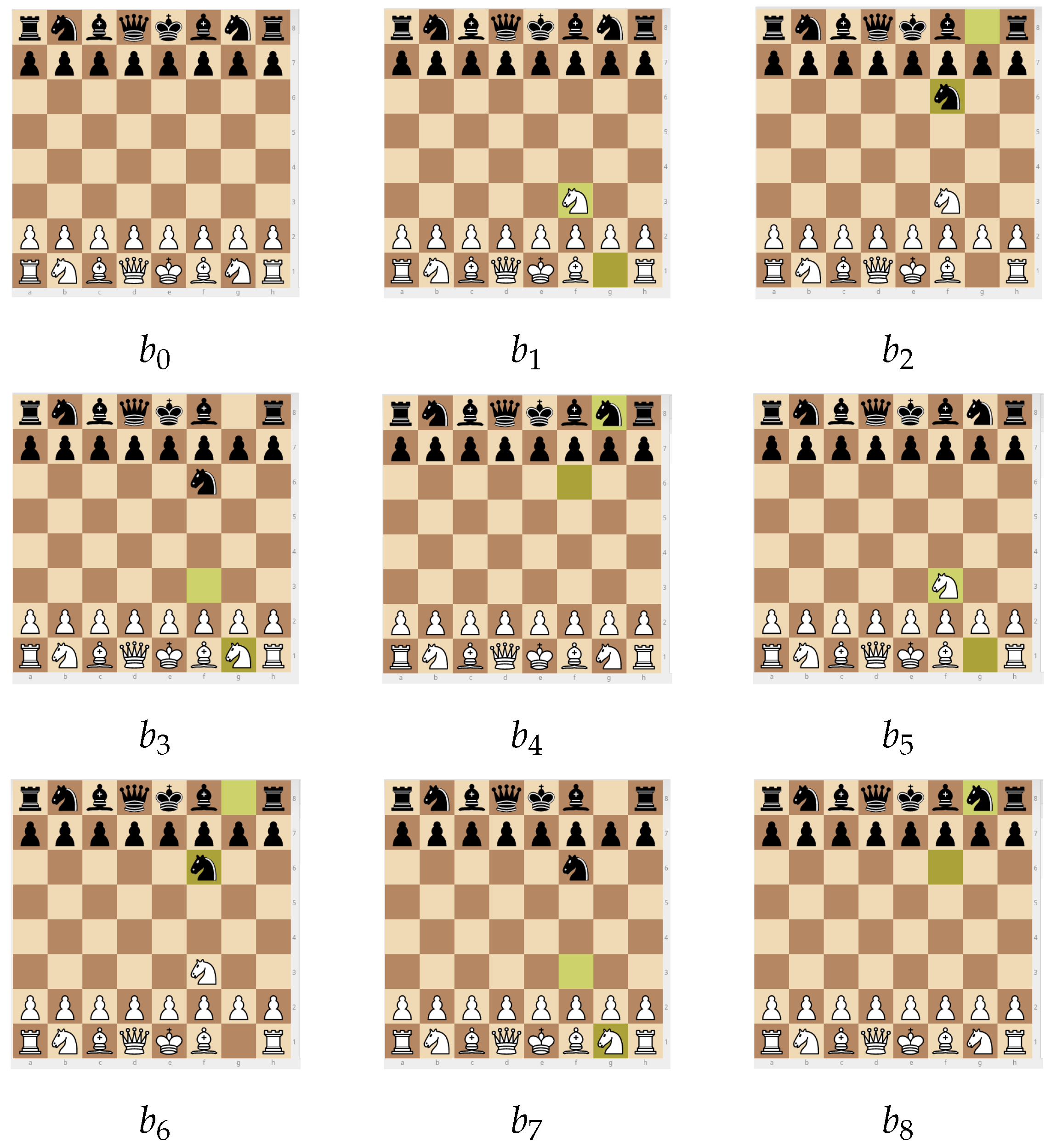
An epoch of a D2PBG is the G-number of all possible valid boards that can be obtained from each board in the previous epoch with exactly one move by the player whose turn it is to play on the boards of the previous epoch. The history of a D2PBG is the G-number of finitely many epochs.

Let $b_0$ be the initial board in Figure 1. Let the history of chess start at epoch

$$E_0=\langle E{M}_0,1\rangle ,$$

(76)

where

$$E{M}_0=\left[\langle \langle \langle 0,b_0\rangle ,0\rangle ,\langle 0,\langle 0,0\rangle \rangle \rangle \right].$$

We observe that

$$\mathtt{s}\mathtt{c}\mathtt{b}\left({\left(l\left(E_0\right)\right)}_1\right)=\mathtt{s}\mathtt{c}\mathtt{b}\left({\left(E{M}_0\right)}_1\right)=b_0$$

and $r\left(E_0\right)=1$ denotes player 1 whose turn it is to play on $\mathtt{s}\mathtt{c}\mathtt{b}\left({\left(l\left(E_0\right)\right)}_1\right)$.

Epoch $E_t$, $t>0$, is

$$E_t=\langle E{M}_t,x\rangle ,$$

(77)

where $E{M}_t$ is pr-computable from $E_{t-1}$ as

$$E{M}_t={\otimes }_r{|}_{m\in l\left(E_{t-1}\right)}\mathtt{m}\mathtt{v}\mathtt{s}(\mathtt{r}\left(E_{t-1}\right),\mathtt{s}\mathtt{c}\mathtt{b}\left(m\right)).$$

(78)

Thus, epoch $E_1$, is pr-computable from $E_0$ as

$$E_1=\langle E{M}_1,2\rangle ,$$

where

$$E{M}_1={\otimes }_r{|}_{m\in l\left(E_0\right)}\mathtt{m}\mathtt{v}\mathtt{s}(1,\mathtt{s}\mathtt{c}\mathtt{b}\left(m\right)).$$

Epoch $E_2$ is pr-computable from $E_1$ as

$$E_2=\langle E{M}_2,1\rangle ,$$

where

$$E{M}_2={\otimes }_r{|}_{m\in l\left(E_1\right)}\mathtt{m}\mathtt{v}\mathtt{s}(2,\mathtt{s}\mathtt{c}\mathtt{b}\left(m\right)).$$

To generalize, we let

$$F_{14}(E_t,t)=\left\{\begin{array}{cc}\langle E{M}_{s\left(t\right)},1\rangle \hfill & \mathrm{if}2\left|s\right(t),\hfill \\ \langle E{M}_{s\left(t\right)},2\rangle \hfill & \mathrm{if}2\nmid s\left(t\right),\hfill \end{array}\right.$$

and define epoch $E_t$ as a primitive recursive function in (79).

$$\begin{array}{ccc}{E}_0\hfill & =\hfill & \langle E{M}_0,1\rangle ,\hfill \\ E_{t+1}\hfill & =\hfill & F_{14}(E_t,t).\hfill \end{array}$$

(79)

Thus,

$$\begin{array}{ccc}& E_0=\langle E{M}_0,1\rangle ;\hfill & \\ & E_1=F_{14}(E_0,0)=\langle E{M}_1,2\rangle ;\hfill & \\ & E_2=F_{14}(E_1,1)=\langle E{M}_2,1\rangle ;\hfill & \\ & E_3=F_{14}(E_2,2)=\langle E{M}_3,2\rangle ;\hfill & \\ & E_4=F_{14}(E_3,3)=\langle E{M}_4,1\rangle ;\hfill & \\ & E_5=F_{14}(E_4,4)=\langle E{M}_5,2\rangle ;\hfill & \\ & \dots \hfill & \end{array}$$

Given an epoch number t, the history of chess, ${\mathbb{H}}_t$, is pr-computable as

$${\mathbb{H}}_t={\otimes }_r{|}_{k=0}^t\left[E_i\right]=[E_0,E_1,\dots ,E_{t-1},E_t].$$

(80)

Thus, for $t>2$.

$$\begin{array}{ccc}{\mathbb{H}}_0\hfill & =\hfill & \left[E_0\right];\hfill \\ {\mathbb{H}}_1\hfill & =\hfill & [E_0,E_1];\hfill \\ {\mathbb{H}}_2\hfill & =\hfill & [E_0,E_1,E_2];\hfill \\ & \dots \hfill & \\ {\mathbb{H}}_t\hfill & =\hfill & [E_0,E_1,E_2,\dots ,E_t].\hfill \end{array}$$

4.12. Games

We define the primitive recursive predicate

$$\mathtt{e}\mathtt{b}(b,t)\equiv (\exists m\in M_t)\{\mathtt{s}\mathtt{c}\mathtt{b}\left(m\right)=b\}$$

(81)

to hold when b is a successor of some move in $M_t$, $t\ge 0$. We will refer to b as an epoch t board. Let the primitive recursive predicate

$$\begin{array}{ccc}\hfill & \mathtt{s}\mathtt{c}\mathtt{r}(b,b^{\prime },t)\equiv \{t>0\wedge \mathtt{e}\mathtt{b}(b,t-1)\wedge \mathtt{e}\mathtt{b}(b^{\prime },t)\wedge \hfill & \\ \hfill & (\exists m\in M_t)\{\mathtt{p}\mathtt{c}\mathtt{b}\left(m\right)=b\wedge \mathtt{s}\mathtt{c}\mathtt{b}\left(m\right)=b^{\prime }\}\}\hfill \end{array}$$

(82)

hold between boards b and $b^{\prime }$ if for some move $m\in M_t$ such that b is the move’s predecessor and $b^{\prime }$ is its successor. In other words, epoch t board $b^{\prime }$ can be obtained from epoch $t-1$ board b in exactly one move by the player whose turn it is to play on b.

Let $z=[b_{i_1},\dots ,b_{i_k}]$, $k\ge 2$, be a sequence of boards and let $b_0$ be the starting board. The primitive recursive predicate

$$\mathtt{h}\mathtt{g}\mathtt{m}\left(z\right)\equiv \mathtt{L}\mathtt{t}\left(z\right)\ge 2\wedge {\left(z\right)}_1=b_0\wedge (\forall t\in \mathtt{g}\mathtt{g}\mathtt{n}(2,\mathtt{L}\mathtt{t}\left(z\right),1))\left\{\mathtt{s}\mathtt{c}\mathtt{r}({\left(z\right)}_{t-1},{\left(z\right)}_t,t)\right\}$$

(83)

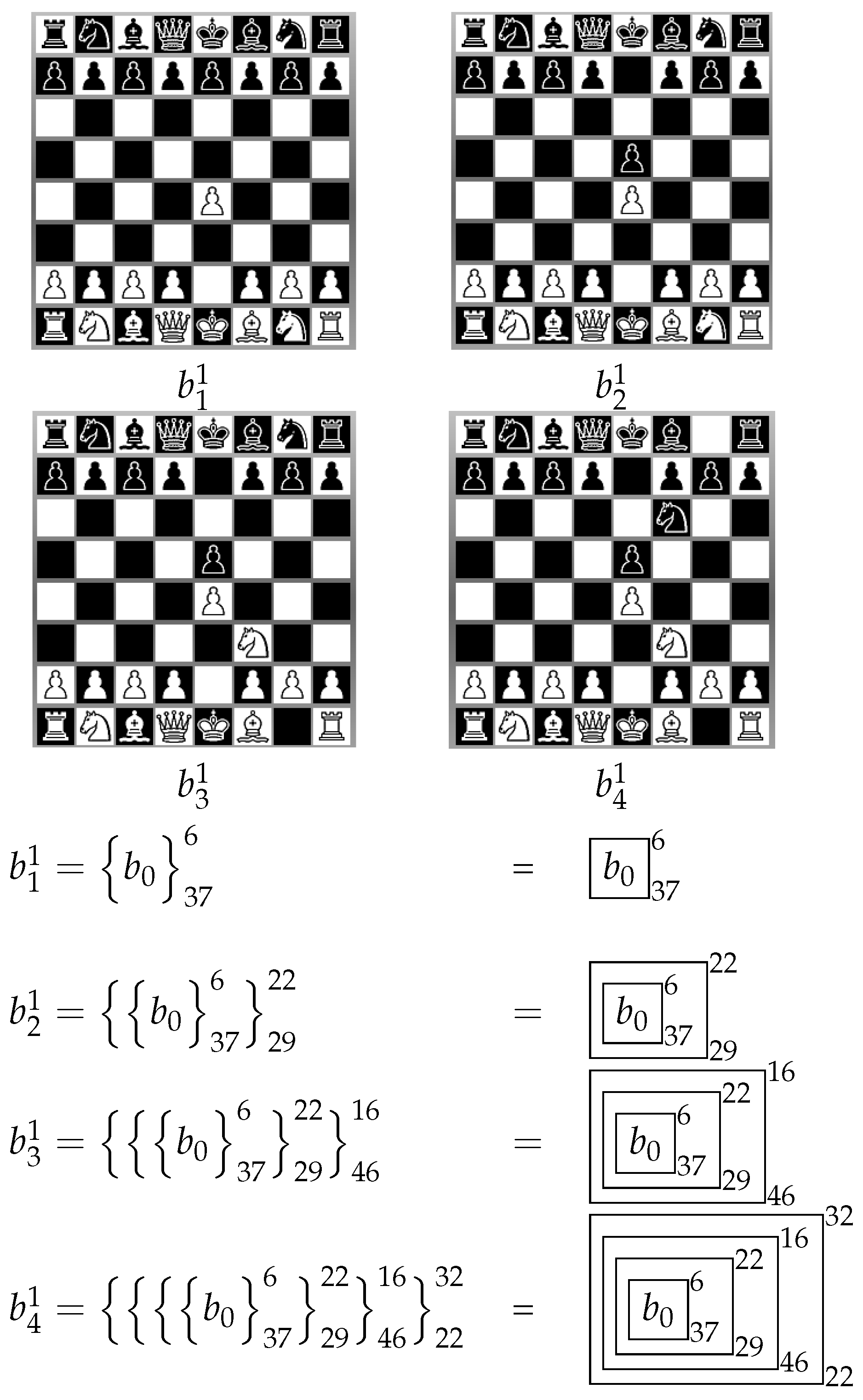
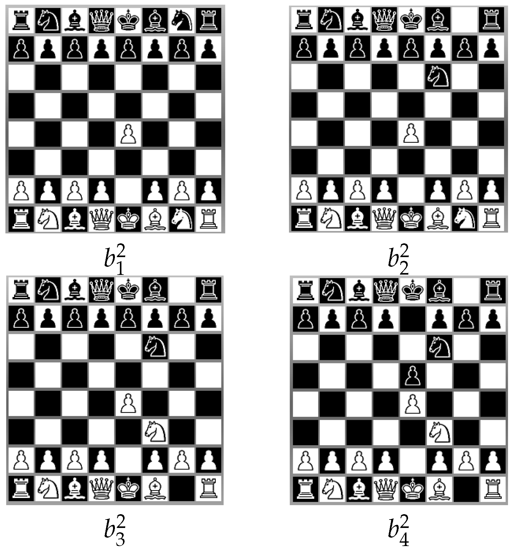
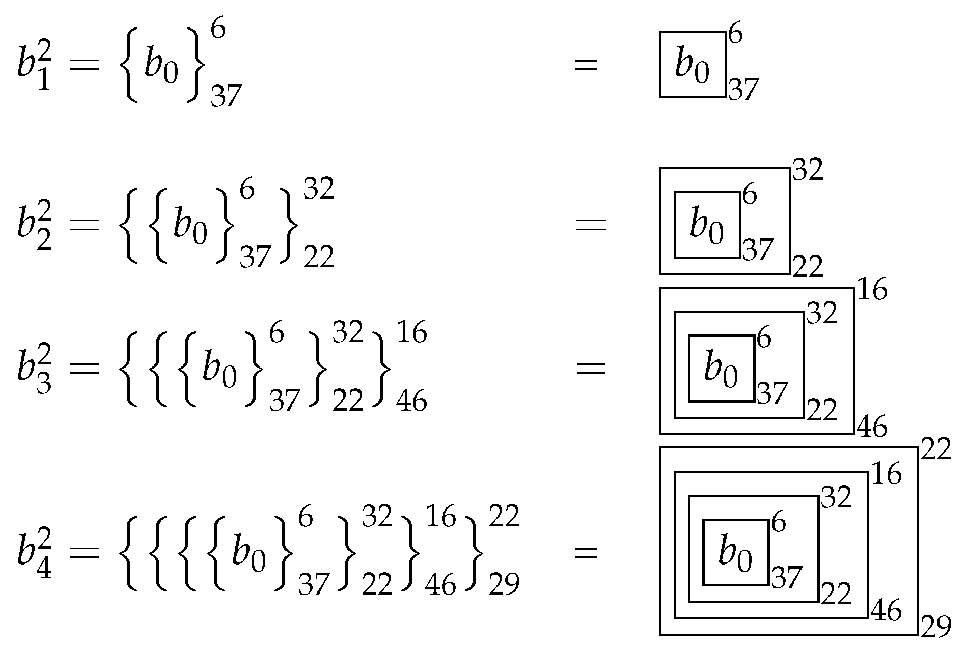
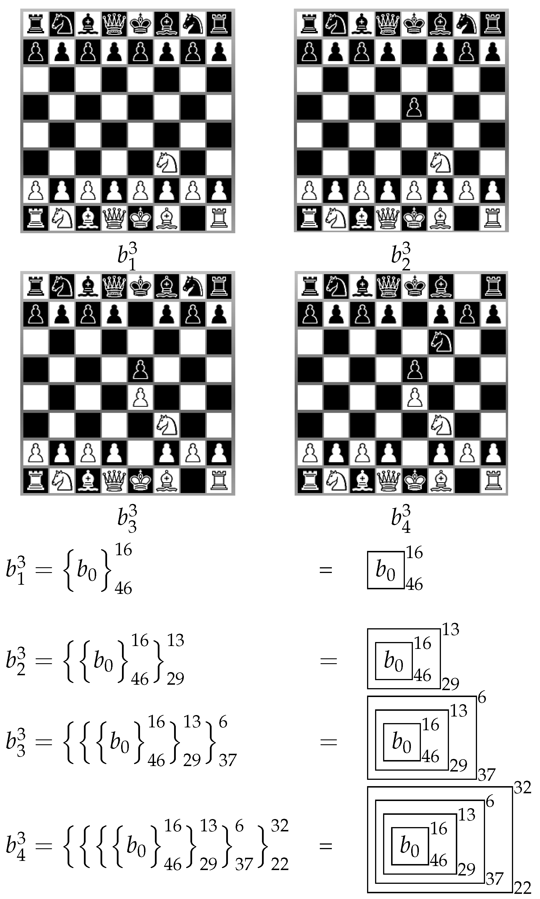
holds of z when it has at least two boards, its first board is $b_0$, and the predicate $\mathtt{s}\mathtt{c}\mathtt{r}(·)$ in (82) holds of every two consecutive boards in z. If $\mathtt{h}\mathtt{g}\mathtt{m}\left(z\right)=1$ for some sequence of boards z, we refer to z as chess game $G_z$ or simply as game $G_z$.

Consider the board sequences in Figure 8, Figure 9, Figure 10 and Figure 11 and let

$$\begin{array}{ccc}& z_1=\left[b_0\right]{\otimes }_r{z}_1^{\prime }=[b_0,b_1^1,b_2^1,b_3^1,b_4^1];\hfill & \\ & z_2=\left[b_0\right]{\otimes }_r{z}_2^{\prime }=[b_0,b_1^2,b_2^2,b_3^2,b_4^2];\hfill & \\ & z_3=\left[b_0\right]{\otimes }_r{z}_3^{\prime }=[b_0,b_1^3,b_2^3,b_3^3,b_4^3];\hfill & \\ & z_3=\left[b_0\right]{\otimes }_r{z}_4^{\prime }=[b_0,b_1^4,b_2^4,b_3^4,b_4^4].\hfill & \end{array}$$

Then, since

$$\mathtt{h}\mathtt{g}\mathtt{m}\left(z_1\right)=\mathtt{h}\mathtt{g}\mathtt{m}\left(z_2\right)=\mathtt{h}\mathtt{g}\mathtt{m}\left(z_3\right)=\mathtt{h}\mathtt{g}\mathtt{m}\left(z_4\right)=1,$$

$G_{z_1}$, $G_{z_2}$, $G_{z_3}$, and $G_{z_4}$ are games.

Let z be a G-number of boards. The primitive recursive function

$$\mathtt{t}\mathtt{l}\mathtt{b}\left(z\right)={\left(z\right)}_{\mathtt{L}\mathtt{t}\left(z\right)}$$

(84)

computes the last board of z. If $G_z$ is a game, we will refer to the last board of $G_z$ (i.e., $\mathtt{t}\mathtt{l}\mathtt{b}\left(G_z\right)$) as the tail board or the tail of $G_z$.

The primitive recursive function $J(·)$ computes the G-number of all games up to epoch $t>0$.

$$\begin{array}{ccc}J\left(0\right)\hfill & =\hfill & \left[\left[b_0\right]\right],\hfill \\ J(t+1)\hfill & =\hfill & F_{15}(J\left(t\right),t),\hfill \end{array}$$

(85)

where

$$F_{15}(Z,t)={\otimes }_r{|}_{z\in Z}{F}_{16}(z,E{M}_{t+1}),$$

(86)

where

$$\begin{array}{ccc}{F}_{16}(z,EM)\hfill & =\hfill & F_{17}(z,{\mathtt{m}\mathtt{a}\mathtt{p}}_{\mathtt{p}\mathtt{c}\mathtt{b}\left(m\right)=\mathtt{t}\mathtt{l}\mathtt{b}\left(z\right)}\left(EM\right),\hfill \\ \hfill & \hfill & \mathtt{L}\mathtt{t}\left({\mathtt{m}\mathtt{a}\mathtt{p}}_{\mathtt{p}\mathtt{c}\mathtt{b}\left(m\right)=\mathtt{t}\mathtt{l}\mathtt{b}\left(z\right)}\left(EM\right)\right)),\hfill \end{array}$$

(87)

where

$$\begin{array}{ccc}{F}_{17}(z,EM,0)\hfill & =\hfill & \left[\right],\hfill \\ F_{17}(z,EM,t+1)\hfill & =\hfill & F_{18}(z,EM,F_{17}(z,EM,t),t),\hfill \end{array}$$

(88)

where

$$F_{18}(z,EM,Z,t)=Z{\otimes }_r\left[z{\otimes }_r\left[\mathtt{s}\mathtt{c}\mathtt{b}\left({\left(EM\right)}_{s\left(t\right)}\right)\right]\right].$$

(89)

The primitive recursive function $F_{18}(·)$ in (89) takes a game $G_z$, a G-number $EM$ of moves such that $(\forall m\in EM)\left\{\mathtt{p}\mathtt{c}\mathtt{b}\right(m)=\mathtt{t}\mathtt{l}\mathtt{b}(z\left)\right\}$, a G-number Z of games and a number t. This function computes the continuation $[z{\otimes }_r\left[\mathtt{s}\mathtt{c}\mathtt{b}\left({\left(EM\right)}_{s\left(t\right)}\right)\right]$ of $G_z$ and appends it at the right of the games Z computed thus far.

The primitive recursive function $F_{17}(·)$ in (88) takes a game $G_z$, a G-number M of moves such that $(\forall m\in EM)\left\{\mathtt{p}\mathtt{c}\mathtt{b}\right(m)=\mathtt{t}\mathtt{l}\mathtt{b}(z\left)\right\}$ and returns the G-number of games each of which is a continuation of $G_z$ with each successor board of the moves $EM$.

The primitive recursive function $F_{16}(·)$ in (87) takes a game $G_z$ and the G-number $EM$ of moves of epoch $t>0$ and computes the G-number of all games that extend $G_z$ with the appropriate successor boards in $EM$ (i.e., with the successor board of each move $m\in EM$ such that $\mathtt{p}\mathtt{c}\mathtt{b}\left(m\right)=\mathtt{t}\mathtt{l}\mathtt{b}\left(z\right)$).

The primitive recursive function $F_{15}(·)$ in (86) takes a G-number of games Z and $t\ge 1$ and computes the G-number of games by extending every game in Z with all appropriate successor boards in $E{M}_{t+1}$. If $t>0$, then

$${\mathbb{G}}_t={\otimes }_r{|}_{i=1}^t\left[J\left(i\right)\right]$$

(90)

is the G-number of all games up to epoch t. All games in ${\mathbb{G}}_t$ are historical in the sense that they are based on the moves in each epoch $E_t$ of ${\mathbb{H}}_t$ in (80). All games in ${\mathbb{G}}_t$ are legal, because they are obtained by legal moves from the initial board $b_0$. We have the following lemma.

Lemma 4.

Let $G_z\in {\mathbb{G}}_t$, $t>0$, and $b=\mathtt{t}\mathtt{l}\mathtt{b}\left(G_z\right)$. Then $\mathtt{L}\mathtt{t}\left(z\right)=t+1$ and if t is even, then player 1 is to play on b; if t is odd, player 2 is to play on b.

Let

$$P_{\mathsf{\Gamma }}\left(z\right)\equiv \mathtt{h}\mathtt{g}\mathtt{m}\left(z\right)\wedge G_z\in {\mathbb{G}}_{\mathtt{L}\mathtt{t}\left(z\right)-1}$$

(91)

be a primitive recursive predicate that holds of z if $G_z$ is a chess game and let

$$\mathsf{\Gamma }=\{z\in \mathbb{N}|P_{\mathsf{\Gamma }}\left(z\right)\}$$

(92)

be the set of numbers for which $P_{\mathsf{\Gamma }}(·)$ holds. Since every primitive recursive function is computable (See Chapter 3 in [5]), we have the following lemma.

Lemma 5.

The set of chess games Γ is recursive.

Lemma 5 shows that the characteristic of chess game historicity or, equivalently, chess game legality is pr-decidable.

Let $G_z$ be a game and let $z^{\prime }$ be a sequence of boards such that $\mathtt{L}\mathtt{t}\left(z^{\prime }\right)>1$. We say that $z^{\prime }$ is a subgame of $G_z$ if the primitive recursive predicate $\mathtt{s}\mathtt{b}\mathtt{g}(·)$ in (93) holds of $G_z$ and $z^{\prime }$.

$$\begin{array}{ccc}\mathtt{s}\mathtt{b}\mathtt{g}(z^{\prime },G_z)\equiv \hfill & \hfill & \\ \{1<\mathtt{L}\mathtt{t}\left(z^{\prime }\right)\le \mathtt{L}\mathtt{t}\left(z\right)\wedge \hfill & \hfill & \\ (\exists i\in \mathtt{g}\mathtt{g}\mathtt{n}(1,\mathtt{L}\mathtt{t}\left(z\right)\dot{-}1,1\left)\right)\{\hfill \\ (\forall k\in \mathtt{g}\mathtt{g}\mathtt{n}(1,\mathtt{L}\mathtt{t}\left(z^{\prime }\right),1))\{{\left(z^{\prime }\right)}_k={\left(z\right)}_{i+k-1}\}\left\}\right\}\hfill \end{array}$$

(93)

In other words, $z^{\prime }$ must have at least 2 boards but no more boards than z and be a sub-sequence of z that starts at some position i between 1 and $\mathtt{L}\mathtt{t}\left(z^{\prime }\right)\dot{-}$1. Consider Figure 10. If

$$z_3=[b_0,b_1^3,b_2^3,b_3^3,b_4^3],$$

then

$$\begin{array}{ccc}\mathtt{s}\mathtt{b}\mathtt{g}([b_0,b_1^3],G_{z_3})\hfill & =\hfill & 1;\hfill \\ \mathtt{s}\mathtt{b}\mathtt{g}([b_1^3,b_2^3,b_3^3],G_{z_3})\hfill & =\hfill & 1;\hfill \\ \mathtt{s}\mathtt{b}\mathtt{g}([b_1^3,b_3^3,b_4^3],G_{z_3})\hfill & =\hfill & 0;\hfill \\ \mathtt{s}\mathtt{b}\mathtt{g}([b_2^3,b_4^3],G_{z_3})\hfill & =\hfill & 0.\hfill \end{array}$$

We define the primitive recursive predicate ${\mathtt{s}\mathtt{b}\mathtt{g}}_2(·)$ to hold when $z^{\prime }$ starts at a specific board i in $G_z$.

$$\begin{array}{cc}{\mathtt{s}\mathtt{b}\mathtt{g}}_2(z^{\prime },G_z,i)\equiv \hfill & \\ \{1<\mathtt{L}\mathtt{t}\left(z^{\prime }\right)\le \mathtt{L}\mathtt{t}\left(z\right)\wedge \{0<i\wedge \hfill \\ (\forall k\in \mathtt{g}\mathtt{g}\mathtt{n}(1,\mathtt{L}\mathtt{t}\left(z^{\prime }\right),1))\{{\left(z^{\prime }\right)}_k={\left(z\right)}_{i+k-1}\}\left\}\right\}\hfill \end{array}$$

(94)

Thus,

$${\mathtt{s}\mathtt{b}\mathtt{g}}_2([b_0,b_1^3],G_{z_3},1)={\mathtt{s}\mathtt{b}\mathtt{g}}_2([b_2^3,b_3^3,b_4^3],G_{z_3},3)=1.$$

4.13. Repetition and 50-Move Rule

We now return to the remaining two types of draw: draw by repetition and the 50-move rule, which we promised to consider at the end of Section 4.9. We recall that a draw by repetition is achieved when the same board position occurs three times in a row with the same player to move. Consider the sequence of boards in Figure 12. Board $b_0$ occurs three times in this sequence (i.e., $b_0=b_4=b_8$) with player 1 to move.

Let $z^{\prime }$ be a subgame with player x to play on ${\left(z^{\prime }\right)}_1$. The same board occurs in a row at ${\left(z^{\prime }\right)}_5$ since x and $\overline{x}$ must make one move each and then reverse that move. Player x then plays on ${\left(z^{\prime }\right)}_5$ and the same board occurs in a row at ${\left(z^{\prime }\right)}_9$, since x and $\overline{x}$ make one move each again and reverse it. Thus, $z^{\prime }$ is a draw by repetition if it has 9 boards such that ${\left(z^{\prime }\right)}_1={\left(z^{\prime }\right)}_5={\left(z^{\prime }\right)}_9$. In other words, if

$$\mathtt{L}\mathtt{t}\left(z^{\prime }\right)=9\wedge {\left(z^{\prime }\right)}_1={\left(z^{\prime }\right)}_5={\left(z^{\prime }\right)}_9.$$

Let $G_z\in {\mathbb{G}}_t$, $t>0$, then $G_z$ is a draw by repetition if

$$\mathtt{d}\mathtt{r}\mathtt{p}\left(G_z\right)\equiv \{\mathtt{L}\mathtt{t}\left(z\right)\ge 9\wedge \mathtt{t}\mathtt{l}\mathtt{b}\left(z\right)={\left(z\right)}_{\mathtt{L}\mathtt{t}\left(z\right)\dot{-}8}={\left(z\right)}_{\mathtt{L}\mathtt{t}\left(z\right)\dot{-}4}\}$$

(95)

The 50-move rule states that a game is a draw when the last 50 moves contain no capture or pawn move. If a game $G_z$ is a draw by the 50-move rule, then $G_z\in {\mathbb{G}}_t$, $t\ge 49$. Let $z^{\prime }$ be a subgame of $G_z$ that has 50 boards (i.e., $\mathtt{L}\mathtt{t}\left(z^{\prime }\right)=50$). Then $G_z$ is a 50-move rule draw if for all boards in $z^{\prime }$ the pawn positions are same and the counts of all white and black pieces remain constant.

We define several auxiliary primitive recursive predicates to compose them into a primitive recursive predicate that holds of $G_z$ if the latter is a draw by the 50-move rule. Let

$$\begin{array}{ccc}& {\zeta }_{\mathtt{w}\mathtt{p}\mathtt{n}}=\mathtt{g}\mathtt{g}\mathtt{n}(2,9,1);\hfill & \\ & {\zeta }_{\mathtt{b}\mathtt{p}\mathtt{n}}=\mathtt{g}\mathtt{g}\mathtt{n}(18,25,1)\hfill & \end{array}$$

be the G-numbers of the white and black pawns, respectively. The primitive recursive predicates $\mathtt{w}\mathtt{p}\mathtt{x}\mathtt{50}(·)$ and $\mathtt{b}\mathtt{p}\mathtt{x}\mathtt{50}(·)$ below hold if every white and black pawn is present or abscent on both boards (i.e., $b_1$ and $b_2$) and, if any white or black pawn is present on both boards, its position is the same on both.

$$\begin{array}{ccc}\hfill & \mathtt{w}\mathtt{p}\mathtt{x}\mathtt{50}(b_1,b_2)\equiv \hfill & \\ \hfill & \left\{(\forall i\in {\zeta }_{\mathtt{w}\mathtt{p}\mathtt{n}})\{\{i\in b_1\wedge i\in b_2\}\vee \{i\notin b_1\wedge i\notin b_2\}\}\right\}\wedge \hfill & \\ \hfill & \left\{(\forall i\in {\zeta }_{\mathtt{w}\mathtt{p}\mathtt{n}})\{\{i\notin b_1\vee i\notin b_2\}\vee \mathtt{c}\mathtt{p}\mathtt{s}\mathtt{n}(i,b_1)=\mathtt{c}\mathtt{p}\mathtt{s}\mathtt{n}(i,b_2)\}\right\}\hfill \end{array}$$

(96)

$$\begin{array}{ccc}\hfill & \mathtt{b}\mathtt{p}\mathtt{x}\mathtt{50}(b_1,b_2)\equiv \hfill & \\ \hfill & \left\{(\forall i\in {\zeta }_{\mathtt{b}\mathtt{p}\mathtt{n}})\{\{i\in b_1\wedge i\in b_2\}\vee \{i\notin b_1\wedge i\notin b_2\}\}\right\}\wedge \hfill & \\ \hfill & \left\{(\forall i\in {\zeta }_{\mathtt{b}\mathtt{p}\mathtt{n}})\{\{i\notin b_1\vee i\notin b_2\}\vee \mathtt{c}\mathtt{p}\mathtt{s}\mathtt{n}(i,b_1)=\mathtt{c}\mathtt{p}\mathtt{s}\mathtt{n}(i,b_2)\}\right\}\hfill \end{array}$$

(97)

We recall that ${\zeta }_{cp}$ in (41) defines the G-number of all the white and black pieces. The primitive recursive predicate

$$\mathtt{c}\mathtt{n}\mathtt{t}\mathtt{x}\mathtt{50}(b_1,b_2)\equiv (\forall j\in {\zeta }_{\mathtt{c}\mathtt{p}})\{\mathtt{c}\mathtt{n}\mathtt{t}(j,b_1)=\mathtt{c}\mathtt{n}\mathtt{t}(j,b_2)\}$$

holds if the counts of all pieces on the boards $b_1$ and $b_2$ are equal.

Let z be a sequence of boards. The primitive recursive predicate

$$\mathtt{w}\mathtt{b}\mathtt{p}\mathtt{50}\left(z\right)\equiv (\forall t\in \mathtt{g}\mathtt{g}\mathtt{n}(1,\mathtt{L}\mathtt{t}\left(z\right)\dot{-}1,1\left)\right)\left\{\mathtt{w}\mathtt{p}\mathtt{x}\mathtt{50}\right({\left(z\right)}_t,{\left(z\right)}_{t+1})\wedge \mathtt{b}\mathtt{p}\mathtt{x}\mathtt{50}({\left(z\right)}_t,{\left(z\right)}_{t+1}\left)\right\}$$

holds if the predicates $\mathtt{w}\mathtt{p}\mathtt{x}\mathtt{50}(·)$ and $\mathtt{b}\mathtt{p}\mathtt{x}\mathtt{50}(·)$ hold for every pair of consecutive boards in z. The primitive recursive predicate

$$\mathtt{c}\mathtt{n}\mathtt{t}\mathtt{50}\left(z\right)\equiv (\forall t\in \mathtt{g}\mathtt{g}\mathtt{n}(1,\mathtt{L}\mathtt{t}\left(z\right)\dot{-}1,1\left)\right)\left\{\mathtt{c}\mathtt{n}\mathtt{t}\mathtt{x}\mathtt{50}\right({\left(z\right)}_t,{\left(z\right)}_{t+1}\left)\right\}$$

holds if the counts of all pieces on all boards in z are equal. The primitive recursive predicate

$$\mathtt{d}\mathtt{r}\mathtt{x}\mathtt{50}\left(z\right)\equiv \mathtt{w}\mathtt{b}\mathtt{p}\mathtt{50}\left(z\right)\wedge \mathtt{c}\mathtt{n}\mathtt{t}\mathtt{50}\left(z\right)$$

holds if the boards in z have no pawn moves or piece captures.

The game $G_z$ is a draw by the 50-move rule if there is a position i in z that starts a subgame of length 50 for which $\mathtt{d}\mathtt{r}\mathtt{x}\mathtt{50}(·)$ holds. The primitive recursive predicate

$$\mathtt{d}\mathtt{r}\mathtt{50}\left(G_z\right)\equiv \mathtt{L}\mathtt{t}\left(z\right)\ge 50\wedge (\exists t\in \mathtt{g}\mathtt{g}\mathtt{n}(1,\mathtt{L}\mathtt{t}\left(z\right)\dot{-}49,1\left)\right)\left\{\mathtt{d}\mathtt{r}\mathtt{x}\mathtt{50}\right(\mathtt{s}\mathtt{s}\mathtt{q}(z,t,t+49)\}$$

(98)

holds if $G_z$ is a draw by the 50-move rule.

4.14. Classification of Games

We define the primitive recursive predicate

$$\mathtt{d}\mathtt{r}\mathtt{g}\left(G_z\right)\equiv \mathtt{d}\mathtt{r}\mathtt{p}\left(G_z\right)\vee \mathtt{d}\mathtt{r}\mathtt{50}\left(G_z\right)\vee \mathtt{b}\mathtt{s}\mathtt{m}\left(\mathtt{t}\mathtt{l}\mathtt{b}\left(G_z\right)\right)\vee \mathtt{w}\mathtt{s}\mathtt{m}\left(\mathtt{t}\mathtt{l}\mathtt{b}\left(G_z\right)\right)\vee \mathtt{d}\mathtt{p}\left(\mathtt{t}\mathtt{l}\mathtt{b}\left(G_z\right)\right)$$

(99)

to hold when $G_z$ is a draw game by repetition, the 50-move rule, stalemate, or dead position. The primitive recursive predicate

$$\mathtt{w}\mathtt{n}\mathtt{g}(G_z,x)\equiv \left\{\begin{array}{cc}\mathtt{b}\mathtt{k}\mathtt{m}\left(\mathtt{t}\mathtt{l}\mathtt{b}\left(G_z\right)\right)\hfill & \mathrm{if}x=1,\hfill \\ \mathtt{w}\mathtt{k}\mathtt{m}\left(\mathtt{t}\mathtt{l}\mathtt{b}\left(G_z\right)\right)\hfill & \mathrm{if}x=2,\hfill \\ 0\hfill & \mathrm{otherwise}\hfill \end{array}\right.$$

(100)

holds when $G_z$ ends in a mate for $\overline{x}$. The primitive recursive predicate

$$\mathtt{u}\mathtt{f}\mathtt{g}(G_z,x)\equiv \neg \mathtt{d}\mathtt{r}\mathtt{g}\left(G_z\right)\wedge \neg \mathtt{w}\mathtt{n}\mathtt{g}(G_z,x)$$

(101)

holds when $G_z$ is unfinished for x (i.e., it is neither a draw nor a win for x).

By Lemma 4, player 1 can win only those games in ${\mathbb{G}}_t$ if t is odd and player 2 can win only games in ${\mathbb{G}}_t$ if t is even. Let $G_z\in {\mathbb{G}}_t$, $t>0$, and let x be the player to play at t. If $G_z$ is not a win for $\overline{x}$, then x can win in 1, 3, 5, …, $2k+1$ moves. Let n be an odd number of moves into the future. We inquire if it is possible to find games $G_y\in {\mathbb{G}}_{t+n}$ that are continuations of $G_z$ and are wins for x in a primitive recursive fashion. The primitive recursive predicate

$$\mathtt{c}\mathtt{n}\mathtt{g}(y,z)\equiv z=\mathtt{s}\mathtt{s}\mathtt{q}(y,1,\mathtt{L}\mathtt{t}\left(z\right))\wedge P_{\mathsf{\Gamma }}\left(y\right)$$

(102)

determines if $G_y$ is a continuation of $G_z$. For any $G_z$, we let the primitive recursive predicate

$$\mathtt{w}\mathtt{c}\mathtt{n}\mathtt{g}(y,x)\equiv \mathtt{c}\mathtt{n}\mathtt{g}(y,z)\wedge \mathtt{w}\mathtt{n}\mathtt{g}(G_y,x)$$

hold when $G_y$ is a continuation of $G_z$ that is a win for x. Let $\mathtt{w}\mathtt{n}\mathtt{x}\left(y\right)\equiv \mathtt{w}\mathtt{c}\mathtt{n}\mathtt{g}(y,1)$ and $\mathtt{b}\mathtt{n}\mathtt{x}\left(y\right)\equiv \mathtt{w}\mathtt{c}\mathtt{n}\mathtt{g}(y,2)$. If $G_z\in {\mathbb{G}}_t$, $t>0$, then the primitive recursive function

$$\mathtt{w}\mathtt{n}\mathtt{g}\mathtt{s}(G_z,x,t,n)=\left\{\begin{array}{cc}{\mathtt{m}\mathtt{a}\mathtt{p}}_{\mathtt{w}\mathtt{n}\mathtt{x}}\left({\mathbb{G}}_{t+n}\right)\hfill & \mathrm{if}2\nmid n\wedge x=1,\hfill \\ {\mathtt{m}\mathtt{a}\mathtt{p}}_{\mathtt{b}\mathtt{n}\mathtt{x}}\left({\mathbb{G}}_{t+n}\right)\hfill & \mathrm{if}2\nmid n\wedge x=2,\hfill \\ 0\hfill & \mathrm{otherwise}\hfill \end{array}\right.$$

(103)

returns the G-number of all continuations of $G_z$ in ${\mathbb{G}}_{t+n}$ that are wins for x whose turn it is to play on the tail of $G_z$. The primitive recursive predicate

$$\mathtt{d}\mathtt{c}\mathtt{n}\mathtt{g}\left(y\right)\equiv \mathtt{c}\mathtt{n}\mathtt{g}(y,z)\wedge \mathtt{d}\mathtt{r}\mathtt{g}\left(G_y\right)$$

holds when $G_y$ is a continuation of $G_z$ that is a draw. If $G_z\in {\mathbb{G}}_t$, $t>0$, then the primitive recursive function

$$\mathtt{d}\mathtt{r}\mathtt{g}\mathtt{s}(G_z,t,n)=\left\{\begin{array}{cc}{\mathtt{m}\mathtt{a}\mathtt{p}}_{\mathtt{d}\mathtt{c}\mathtt{n}\mathtt{g}}\left({\mathbb{G}}_{t+n}\right)\hfill & \mathrm{if}2\nmid n,\hfill \\ 0\hfill & \mathrm{otherwise}\hfill \end{array}\right.$$

(104)

returns the G-number of all continuations of $G_z$ in ${\mathbb{G}}_{t+n}$ that are draws for x whose turn it is to play on the last board of $G_z$. The primitive recursive predicate

$$\mathtt{u}\mathtt{c}\mathtt{n}\mathtt{g}(y,x)\equiv \mathtt{c}\mathtt{n}\mathtt{g}(y,z)\wedge \mathtt{u}\mathtt{f}\mathtt{g}(G_y,x)$$

holds when $G_y$ is a continuation of $G_z$ that is unfinished for x. Let $\mathtt{w}\mathtt{u}\mathtt{x}\left(y\right)\equiv \mathtt{u}\mathtt{c}\mathtt{n}\mathtt{g}(y,1)$ and $\mathtt{b}\mathtt{u}\mathtt{x}\left(y\right)\equiv \mathtt{u}\mathtt{c}\mathtt{n}\mathtt{g}(y,2)$. If $G_z\in {\mathbb{G}}_t$, $t>0$, then the primitive recursive function

$$\mathtt{u}\mathtt{f}\mathtt{g}\mathtt{s}(G_z,x,t,n)=\left\{\begin{array}{cc}{\mathtt{m}\mathtt{a}\mathtt{p}}_{\mathtt{w}\mathtt{u}\mathtt{x}}\left({\mathbb{G}}_{t+n}\right)\hfill & \mathrm{if}2\nmid n\wedge x=1,\hfill \\ {\mathtt{m}\mathtt{a}\mathtt{p}}_{\mathtt{b}\mathtt{u}\mathtt{x}}\left({\mathbb{G}}_{t+n}\right)\hfill & \mathrm{if}2\nmid n\wedge x=2,\hfill \\ 0\hfill & \mathrm{otherwise}\hfill \end{array}\right.$$

(105)

returns the G-number of all continuations of $G_z$ in ${\mathbb{G}}_{t+n}$ that are unfinished for x whose turn it is to play on the tail of $G_z$.

Let $G_z\in {\mathbb{G}}_t$, $t>0$, and let x be the player whose turn it is to play on the tail of $G_z$. We will further assume that $G_z$ is unfinished (i.e., $\mathtt{u}\mathtt{f}\mathtt{g}(G_z,x)=1$) for x. We call $G_z$winnable for x in n moves if $\mathtt{w}\mathtt{n}\mathtt{g}\mathtt{s}(G_z,x,t,n)\ne 0$, drawable for x in n moves if $\mathtt{d}\mathtt{r}\mathtt{g}\mathtt{s}(G_z,t,n)\ne 0$, and unfinishable for x in n moves if $\mathtt{u}\mathtt{f}\mathtt{g}\mathtt{s}(G_z,x,t,n)\ne 0$. We will call unfinishable games hangs. If a player makes a move that results in a hang, we will say that the player hangs the game or that the game is hung. We have the following lemma.

Lemma 6.

Let $G_z\in {\mathbb{G}}_t$, $t>0$, be a hang and x be the player whose turn it is to play on $b=\mathtt{t}\mathtt{l}\mathtt{b}\left(z\right)$. If n is an odd positive integer, then it is pr-decidable whether $G_z$ is is winnable for x within n moves, is drawable for x within n moves, or is a hang for x within n moves.

Of course, if a game is winnable, drawable, or unfinishable for x, x may still lose it within n moves, because there may be a sequence of at most n moves from the tail of $G_z$ that allows $\overline{x}$ to win.

We pose the question if it is pr-decidable to whether $G_z$ is absolutely winnable for x within n moves when x is to play on the tail of $G_z$. $G_z$ is absolutely winnable for x if any continuation of $G_z$ of less than or equal to n boards results in a win for x and is not winnable or drawable for $\overline{x}$.

Let us assume that $G_z\in {\mathbb{G}}_t$, $t>0$, and x is the player whose turn it is to play on the tail of $G_z$ and $G_z$ is unfinished (i.e., $\mathtt{u}\mathtt{f}\mathtt{g}(G_z,x)=0$). Let

$$\begin{array}{ccc}\hfill & g_1=\mathtt{g}\mathtt{g}\mathtt{n}(t+1,t+n,2)\hfill & \\ \hfill & g_2=\mathtt{g}\mathtt{g}\mathtt{n}(t+2,t+n,2)\hfill & \end{array}$$

(106)

be the G-numbers of game epochs strictly between t and $t+n$, where $g_1=[(t+1),(t+1)+2,\dots ,(t+1)+2j]$, and $g_2=[t+2,t+2·2,\dots ,t+2k]$, where $(t+1)+2j$ and $t+2k$ are the largest numbers less than $t+n$ obtained in even increments from $(t+1)$ and $(t+2)$, respectively. G-number $g_1$ contains the numbers of epochs, where $\overline{x}$ plays and x can win, draw, or hang, and $g_2$ contains the numbers of epochs where x plays and $\overline{x}$ can win, draw, or hang.

The primitive recursive predicate

$${\mathtt{a}\mathtt{w}\mathtt{g}}_1(G_z,x,n)\equiv (\forall t\in g_1)(\forall y\in {\mathbb{G}}_t)\{\neg \mathtt{c}\mathtt{n}\mathtt{g}(y,z)\vee \mathtt{w}\mathtt{c}\mathtt{n}\mathtt{g}(y,x)\}$$

holds if x wins every continuation $G_y$ of $G_z$ within n moves and the primitive recursive predicate

$${\mathtt{a}\mathtt{w}\mathtt{g}}_2(G_z,x,n)\equiv (\forall t\in g_2)(\forall y\in {\mathbb{G}}_t)\{\neg \mathtt{c}\mathtt{n}\mathtt{g}(y,z)\vee \mathtt{u}\mathtt{c}\mathtt{n}\mathtt{g}(y,\overline{x})\}$$

holds if every continuation $G_y$ of $G_z$ within n moves is a hang for $\overline{x}$.

The primitive recursive predicate

$$\mathtt{a}\mathtt{w}\mathtt{g}(G_z,x,n)\equiv {\mathtt{a}\mathtt{w}\mathtt{g}}_1(G_z,x,n)\wedge {\mathtt{a}\mathtt{w}\mathtt{g}}_2(G_z,x,n)$$

(107)

holds if $G_z$ is absolutely winnable for x within n moves.

Is it pr-decidable if x can win or draw $G_z$ from its tail within the next n moves while $\overline{x}$ cannot win under any sequence of moves less than or equal to n? If $G_z$ is such a game, we call it favorable for x.

We define the primitive recursive predicate

$${\mathtt{f}\mathtt{v}\mathtt{g}}_1(G_z,x,n)\equiv (\forall t\in g_1)(\forall y\in {\mathbb{G}}_t)\{\neg \mathtt{c}\mathtt{n}\mathtt{g}(y,z)\vee \{\mathtt{d}\mathtt{c}\mathtt{n}\mathtt{g}\left(y\right)\vee \mathtt{w}\mathtt{c}\mathtt{n}\mathtt{g}(y,x)\}\}$$

to hold if x wins or draws in every continuation $G_y$ of $G_z$ within n moves and define the primitive recursive predicate

$${\mathtt{f}\mathtt{v}\mathtt{g}}_2(G_z,x,n)\equiv (\forall t\in g_2)(\forall y\in {\mathbb{G}}_t)\{\neg \mathtt{c}\mathtt{n}\mathtt{g}(y,z)\vee \mathtt{u}\mathtt{c}\mathtt{n}\mathtt{g}(y,\overline{x})\}$$

to hold if every continuation $G_y$ of $G_z$ within n moves is a hang for $\overline{x}$.

The primitive recursive predicate

$$\mathtt{f}\mathtt{v}\mathtt{g}(G_z,x,n)\equiv {\mathtt{f}\mathtt{v}\mathtt{g}}_1(G_z,x,n)\wedge {\mathtt{f}\mathtt{v}\mathtt{g}}_2(G_z,x,n)$$

(108)

holds if $G_z$ is favorable for x within n moves in that in any continuation $G_y$ of $G_z$ within the next n moves x wins or draws whereas $\overline{x}$ hangs.

Is it pr-decidable whether neither x nor $\overline{x}$ can win or draw $G_z$ within the next n moves from the tail of $G_z$? In other words, is any continuation of $G_z$ within the next n moves from its tail is a hang? If that it the case, let us refer to $G_z$ as an absolute hang or absolutely unfinishable.

The primitive recursive predicate

$${\mathtt{a}\mathtt{h}\mathtt{g}}_1(G_z,x,n)\equiv (\forall t\in g_1)(\forall y\in {\mathbb{G}}_t)\{\neg \mathtt{c}\mathtt{n}\mathtt{g}(y,z)\vee \mathtt{u}\mathtt{c}\mathtt{n}\mathtt{g}(y,x)\}$$

holds if x hangs in every continuation $G_y$ of $G_z$ within n moves, and the primitive recursive predicate

$${\mathtt{a}\mathtt{h}\mathtt{g}}_2(G_z,x,n)\equiv (\forall t\in g_2)(\forall y\in {\mathbb{G}}_t)\{\neg \mathtt{c}\mathtt{n}\mathtt{g}(y,z)\vee \mathtt{u}\mathtt{c}\mathtt{n}\mathtt{g}(y,\overline{x})\}$$

holds if every continuation $G_y$ of $G_z$ within n moves is a hang for $\overline{x}$.

The primitive recursive predicate

$$\mathtt{a}\mathtt{h}\mathtt{g}(G_z,x,n)\equiv {\mathtt{a}\mathtt{h}\mathtt{g}}_1(G_z,x,n)\wedge {\mathtt{a}\mathtt{h}\mathtt{g}}_2(G_z,x,n)$$

(109)

holds if $G_z$ is unfinishable for x and $\overline{x}$ within n moves.

We summarize the above arguments in the following lemma.

Lemma 7.

Let $G_z\in {\mathbb{G}}_t$, $t>0$, be a hang and x be the player whose turn it is to play on $b=\mathtt{t}\mathtt{l}\mathtt{b}\left(z\right)$. If n be an odd positive integer, then it is pr-decidable whether $G_z$ is absolutely winnable for x within n moves, is favorable for x within n moves, or is an absolute hang for x (and $\overline{x}$) within n moves.

Before we leave this section, we summarize our findings in the following lemma.

Lemma 8.

The following characteristics of chess are pr-decidable: board validity, checkmate, stalemate, draw, potential and actual reachability, game winnability, drawability, and unfinishability within the next n moves, absolute game winnability and unfinishability within the next n moves and game favorability within the next n moves, where n is a positive odd integer.

5. Procedures

Suppose $G_z\in {\mathbb{G}}_t$, $t>0$, and the player x is to play on the tail of $G_z$. Is an optimal continuation of $G_z$ for x within n moves pr-computable for some positive odd n? An optimal continuation may be the continuation of 0 moves (i.e., resignation), which is the only rational decision in the absence of any wins or draws. Lemma 8 suggests a host of primitive recursive procedures for x to find an optimal continuation including the resignation. If $\mathtt{a}\mathtt{w}\mathtt{g}(G_z,x,n)$ is true, then let

$$Z_a=\mathtt{w}\mathtt{n}\mathtt{g}\mathtt{s}(G_z,x,t,n)$$

be the pr-computable G-number of winnable games for x within n moves, which, since $G_z$ is absolutely winnable, includes all continuations of $G_z$ within n moves. The next move from ${\left(Z_a\right)}_1$ can be arbitrarily chosen for x to play (e.g., ${\left({\left(Z_a\right)}_1\right)}_{\mathtt{L}\mathtt{t}\left(z\right)+1})$. Alternatively, the minimalization can be used to find the index of $z^{\prime }\in Z_a$ such that

$$(\forall z^{\prime \prime }\in Z_a)\{z^{\prime }=z^{\prime \prime }\vee \mathtt{L}\mathtt{t}\left(z^{\prime }\right)\le \mathtt{L}\mathtt{t}\left(z^{\prime \prime }\right)\}.$$

Since the above predicate is primitive recursive, so is its minimalization. If $G_{z^{\prime }}$ is the shortest absolutely winnable game found through the minimalization of the above primitive recursive predicate, the next move is chosen as

$${\left(z^{\prime }\right)}_{\mathtt{L}\mathtt{t}\left(z\right)+1}.$$

If $\mathtt{a}\mathtt{w}\mathtt{g}(G_z,x,n)=0$ but $\mathtt{f}\mathtt{v}\mathtt{g}(G_z,x,n)=1$, then let

$$\begin{array}{ccc}{Z}_w\hfill & =\hfill & \mathtt{w}\mathtt{n}\mathtt{g}\mathtt{s}(G_z,x,t,n);\hfill \\ Z_d\hfill & =\hfill & \mathtt{d}\mathtt{r}\mathtt{g}\mathtt{s}(G_z,x,t,n).\hfill \end{array}$$

Since $G_z$ is favorable, all continuations of $G_z$ within the next n moves will be in $Z_w$ or $Z_d$. If $Z_w\ne 0$, x uses the minimalization to find the shortest continuation in $Z_w$ as outlined above and selects the next move from that continuation. If $Z_w=0$, then all continuations of $G_z$ are draws for x within the next n moves, and x can choose the next move from the shortest continuation in $Z_d$. If $\mathtt{a}\mathtt{w}\mathtt{g}(G_z,x,n)=\mathtt{f}\mathtt{v}\mathtt{g}(G_z,x,n)=0$ but $\mathtt{a}\mathtt{h}\mathtt{g}(G_z,x,n)=1$, then x chooses the next move from the shortest z in

$$Z_h=\mathtt{u}\mathtt{f}\mathtt{g}\mathtt{s}(G_z,x,t,n).$$

What if $Z_w=Z_d=Z_h=0$? In this case, $G_z$ is absolutely losable or an absolute loss for x within n moves. The primitive recursive predicate

$$\begin{array}{ccc}\mathtt{a}\mathtt{l}\mathtt{g}(G_z,x,n)\hfill & \equiv \hfill & \mathtt{w}\mathtt{n}\mathtt{g}\mathtt{s}(G_z,x,\mathtt{L}\mathtt{t}\left(z\right)+1,n)\hfill \\ \hfill & =\hfill & \mathtt{d}\mathtt{r}\mathtt{g}\mathtt{s}(G_z,x,\mathtt{L}\mathtt{t}\left(z\right)+1,n)\hfill \\ \hfill & =\hfill & \mathtt{u}\mathtt{f}\mathtt{g}\mathtt{s}(G_z,x,\mathtt{L}\mathtt{t}\left(z\right)+1,n)\hfill \\ \hfill & =\hfill & 0\hfill \end{array}$$

(110)

holds when $G_z$ is absolutely losable for x within the next n moves. In this case, the concept of lookahead (i.e., $n+m$ moves ahead for some positive even number m) can be applied and the above primitive recursive steps of computing $Z_w$, $Z_d$, and $Z_h$ repeated so long as $n+m\le K$, where K is some arbibrary large positive odd integer. Taking $M=399$ should suffice in light of the fact that the longest game so far in the history of chess took 269 moves to complete and lasted 20 h and 15 min [8]. If $G_z$ remains absolutely losable for x within the next K moves, x resigns.

What if $Z_h\ne 0$ (i.e., there are absolute hangs)? We can use the same incremental lookahead method to determine if any $G_{z^{\prime }}\in Z_h$ is absolutely winnable or favorable for x within the next K moves. If there is an absolutely winnable game, x plays the first move of that game. If there is a favorable game, x plays the first move of that game.

If there are no absolutely winnable or favorable games within the next K moves for any game in $Z_h$, it must be decided for x which unfinishable game in $Z_h$ to choose. One possible pr-computable procedure is to choose a continuation $G_{z^{\prime }}$ of $G_z$ in $Z_h$ for which the counts of the pieces for each board of $G_{z^{\prime }}$ are equal. If there is such a game, x plays its first move.

Another, more flexible, pr-computable procedure is to assign an arbitrary value (a positive integer) to each piece: 2 to a pawn, 3 to a knight and a bishop, 5 to a rook, 7 to a queen and compute the value of each board for player x as the sum of x’s pieces on the board. Then a continuation $G_{z^{\prime }}\in Z_h$ of $G_z$ is chosen where each board from the tail of $G_z$ to the tail of $G_{z^{\prime }}$ has the same value for x and $\overline{x}$ or the difference in the values does not exceed an arbitrarily chosen number. In general, any decision procedure or a utility function that is built from primitive recursive functions and predicates that compute properties of G-numbers will be primitive recursive.

The above discussion furnishes us with the following theorem and a corollary.

Theorem 1.

Let $G_z\in {\mathbb{G}}_t$, $t>0$, be a hang and x be the player whose turn it is to play on $b=\mathtt{t}\mathtt{l}\mathtt{b}\left(z\right)$ and let K be a large positive odd integer. Then there exist pr-computable procedures to compute optimal continuations of $G_z$ for x and to decide if $G_z$ is absolutely losable for x within the next M moves.

Corollary 1.

Absolute losability of a chess game is a pr-decidable characteristic.

6. Discussion

In the AI game playing literature (e.g., [9,10]), game engines are functions computed by programs that can play specific games by generating legal moves against humans or other programs with varying degrees of success. These programs almost never compute total functions, because they are based on search control heuristics (e.g., A*, minimax, alpha-beta pruning, etc.). Thus, even when their inputs and outputs can be represented as natural numbers with a rigorous Gödel numbering scheme, they can be construed only as partially computable functions. Furthermore, programs that play games with difficult combinatorics (chess, checkers, Go, etc.) break the fundamental tenet of classical computability in Rogers’ quote from [4] in Section 1, because, to be efficient, they must estimate, ahead of computation, how long the decision making process takes and heuristically prune continuations.

In the classification of Barr and Feigenbaum [9], D2PBGs are games that can be represented with AND/OR trees. Specifically, Barr and Feigenbaum write that

‘‘[a]t each turn, the rules define both what moves are legal

and the effect that each possible move will have; there is

no element of chance. In contrast to card games in which the

players’ hands are hidden, each player has complete information

about his opponent’s position, including the choices open to

him and the moves he has made. The game begins from a specified

state, often a configuration of men on a board. It ends in a

win for one player and a loss for the other, or possibly in

a draw.’’

Russell and Norvig [10] characterize chess as “a game of perfect information”, because “the agent can perceive everything there is to know about the environment”. In our opinion, Russell and Norvig’s definition is less precise than Barr and Feigenbaum’s, because it appears to separate computation and perception. If perception is not computation, then AI D2PBG engines fall outside of the scope of classical computability. If perception is computation, many such engines are partially computable functions, because they are not total due to heuristic pruning.

AND/OR game trees can be searched with minimax [9]. If in a chess engine both players use minimax on the complete AND/OR game tree, which is feasible only in theory, and if the board evaluation function applied to each tree node by each player is primitive recursive, then the engine is a primitive recursive function by Lemma 8 and the Section 5 theorem. However, if the board evaluation function in minimax is not primitive recursive (e.g., if it is computable but not primitive recursive or partially computable), then the engine is not primitive recursive.

What if we put aside heuristic search control (e.g., minimax) and consider a chess game engine that uses an artificial or convolutional neural network (ANN or ConvNet) (e.g., [11])? In this case, the chess engine computes a primitive recursive function if and only if the synapse weights are natural numbers, which is never the case in the state-of-the-art ANNs or ConvNets that play such games as chess and Go. They are deep multi-layer networks where each weight is a real number (typically, but not always, between 0 and 1). But, since there are uncountably many reals between 0 and 1 or in any interval defined by two distinct real numbers, it is impossible to generate network states with primitive recursion. Consequently, if the chess engine is a ANN/ConvNet, then the engine may be computable, but not primitive recursive. Of course, even the computability of the engine depends on whether, in addition to representing inputs and outputs as natural numbers, we are able to show that the engine computes a total function.

Any characteristic of a D2PBG game with a finite history (e.g., Tic Tac Toe) is pr-decidable and pr-computable in the sense that the entire game history is a G-number and an optimal sequence of moves for either player can be found using number-theoretic methods from an arbitrary board within that number.

A D2PBG all of whose boards can be calculated in a primitive recursive fashion within the next K moves for some arbitrarily large number K (with the magnitude of K dependent on the rules of the game) is pr-decidable for K in the sense that for either player it is possible to decide in a primitive recursive fashion whether an unfinished game is absolutely winnable, favorable, or absolutely losable within K moves. If a game is absolutely unfinishable within the next K moves, then there exist primitive recursive calculation procedures to choose the next move and in that sense (and that sense only) chess is pr-computable.

As we showed in this article, some characteristics of chess are pr-computable. Any characteristic of the chess board (and, in general, a board in a D2PBG) represented as a G-number that can be decided by a primitive recursive predicate through primitive recursive number-theoretic methods is pr-decidable. Since sequences of boards can be combined into G-numbers as games, any characteristic of the G-number of a game that can be calculated through primitive recursive number-theoretic methods is pr-computable and pr-decidable.

The following questions remain open with respect to chess as a D2PBG:

• Is chess a D2PBG with a finite history? In other words, is there $t>0$ such that $(\forall t^{\prime })\{t^{\prime }\le t\vee E_{t^{\prime }}=0\}$? (See Equation (79)).
• Are there computable decision procedures for player x that are not primitive recursive and that guarantee for x to win or draw an unfinished game if $\overline{x}$ uses only primitive recursive decision procedures?
• Are there games that x cannot lose when x uses only primitive recursive decision procedures while $\overline{x}$ uses computable decision procedures that are not primitive recursive?

7. Summary

We investigated several characteristics of chess with methods of computability and number theories. We showed that chess boards can be represented as Gödel numbers (G-numbers). The following characteristics were shown to be pr-decidable: board validity, position reachability, potential and actual position reachability, check, mate, stalemate, and draw.

We showed that it is pr-decidable whether an unfinished game is absolutely winnable, favorable (i.e., winnable or drawable), or absolutely losable within a specified number of moves for the player whose turn it is to play on the last board. We also showed that that there exist primitive recursive procedures to compute optimal continuations of an unfinished game and that the set of all chess games is recursive.