Article

Stochastic Bifurcations and Excitement in the ZS-Model of a Thermochemical Reaction

Institute of Natural Sciences and Mathematics, Ural Federal University, 620000 Ekaterinburg, Russia
*
Author to whom correspondence should be addressed.
Mathematics 2022, 10(6), 960; https://doi.org/10.3390/math10060960
Submission received: 14 February 2022 / Revised: 14 March 2022 / Accepted: 16 March 2022 / Published: 17 March 2022

Abstract

:
The Zeldovich–Semenov model of the continuous stirred tank reactor with parametric random disturbances in temperature is considered. We study a phenomenon of noise-induced transformation of the equilibrium mode into the mixed-mode oscillatory stochastic regime with alternations between small and large amplitudes. In the parametric analysis of the stochastic excitement, we use the analytical method of confidence domains based on the stochastic sensitivity technique. Analyzing a mutual arrangement of the confidence ellipses and separatrices, we estimate the critical intensity of the noise that causes the excitation. The phenomena of stochastic P-bifurcations and coherence resonances are discovered and studied by probability density functions and the statistics of interspike intervals.

1. Introduction

At present, mathematical modeling is widely used in studying the mechanisms of various complex combustion processes. The strong nonlinearity of the thermochemical models (see, e.g., [1,2,3]) gives rise to variability in the dynamic modes, both equilibrium and oscillatory. In these circumstances, a modern bifurcation theory of nonlinear dynamic systems is a basic tool of mathematical analysis. In these investigations, the Zeldovich–Semenov (ZS) model [4,5,6] of the continuous stirred tank reactor (CSTR) is actively used [1,7,8]. To date, the detailed parametric analysis of the deterministic ZS model has been carried out [9,10]. In real combustion processes, random disturbances are an inevitable attribute. So, an elaboration of methods of the analysis for stochastic thermochemical models is a challenging problem of applied nonlinear dynamics.
It is well-known that the noise in nonlinear systems can drastically change initial deterministic behaviors and cause various stochastic phenomena, e.g., stochastic bifurcations [11,12,13], noise-induced transitions [14,15,16], stochastic and coherence resonances [17,18,19], noise-induced phantom attractors [20,21], stochastic excitability [22,23,24], noise-induced chaos-order transformations [25,26,27], etc. In the parametric studies of these phenomena, methods of approximation of probabilistic distributions in randomly forced attractors are actively elaborated [28,29,30]. A useful tool here is the technique of stochastic sensitivity [31,32,33] and confidence regions [27,34,35]. This technique is successfully applied to the mathematical analysis of noise-induced phenomena in various fields of science [36,37,38].
This paper aims to study probabilistic mechanisms of stochastic phenomena in the Zeldovich–Semenov model with random multiplicative disturbances in the temperature of CSTR. While the deterministic variant of the model is well studied, our paper shows for the first time how, under the action of even small noise, equilibrium modes are deformed into oscillatory spiking regimes. We not only register this phenomenon of stochastic excitement but also suggest a mathematical method for its analysis using the author’s technique of stochastic sensitivity.
In Section 2, we briefly overview the bifurcations and attractors of the initial deterministic ZS model. Here, we emphasize peculiarities of the deterministic behavior (non-uniformity, pseudo-separatrices, transients) that are important for the analysis of stochastic excitability. Section 3 is devoted to the description and probabilistic analysis of stochastic effects in the ZS model with random parametric disturbances. Here, the phenomenon of a noise-induced transition from an equilibrium regime to mixed-mode oscillations is studied both numerically and theoretically. Our analysis is based on the confidence ellipses method. Amplitude changes in the generated spiking oscillations are investigated by probability densities. Here, stochastic P-bifurcations are discussed. We analyze the statistics of interspike intervals in the study of frequency changes for noise-induced mixed-mode oscillations. For the ZS model with parametric random disturbances, we first reveal the phenomenon of coherence resonance.

2. Deterministic Model

In this paper, as the initial deterministic skeleton, we use the mathematical Zeldovich–Semenov model of a thermochemical reaction [10]:
x ˙ = ( 1 x ) exp y 1 + β y x D γ y ˙ = ( 1 x ) exp y 1 + β y y S .
This system describes a dynamical interaction of two variables: the concentration x of the reagent and the temperature y in the reactor. Positive parameters β , γ , S , and D define the kinetics of the reaction. In our paper, following [10], we fix β = 0.05 , γ = 0.03 , S = 0.7 , and study the system (1) dynamics under variation of the parameter D.
The key regimes of the system behavior are presented in Figure 1, where the bifurcation diagram is shown. Here, extreme values of x- and y-coordinates of the system attractors are plotted by solid lines.
The system (1) has the equilibrium M ( x ¯ , y ¯ ) with coordinates satisfying the following system:
( S D y ) exp y 1 + β y = y , x = D S y .
Changes in the system dynamics are connected with three bifurcation points: D 1 = 0.104 , D 2 = 0.241 , and D 3 = 0.2471004 .
For D < D 1 , the equilibrium M is stable. As the parameter D passes the Andronov–Hopf supercritical bifurcation point D 1 , this equilibrium loses its stability, and the stable limit cycle Γ appears. This cycle is stable in the interval D 1 < D < D 3 and disappears at the saddle-node bifurcation point D 3 . The equilibrium M is unstable in the interval D 1 < D < D 2 (see red dashed line in Figure 1) and stable for D > D 2 . Here, D 2 is the point of the subcritical bifurcation. So, for D 2 < D < D 3 , the system (1) is bistable with coexisting equilibrium M and limit cycle Γ .
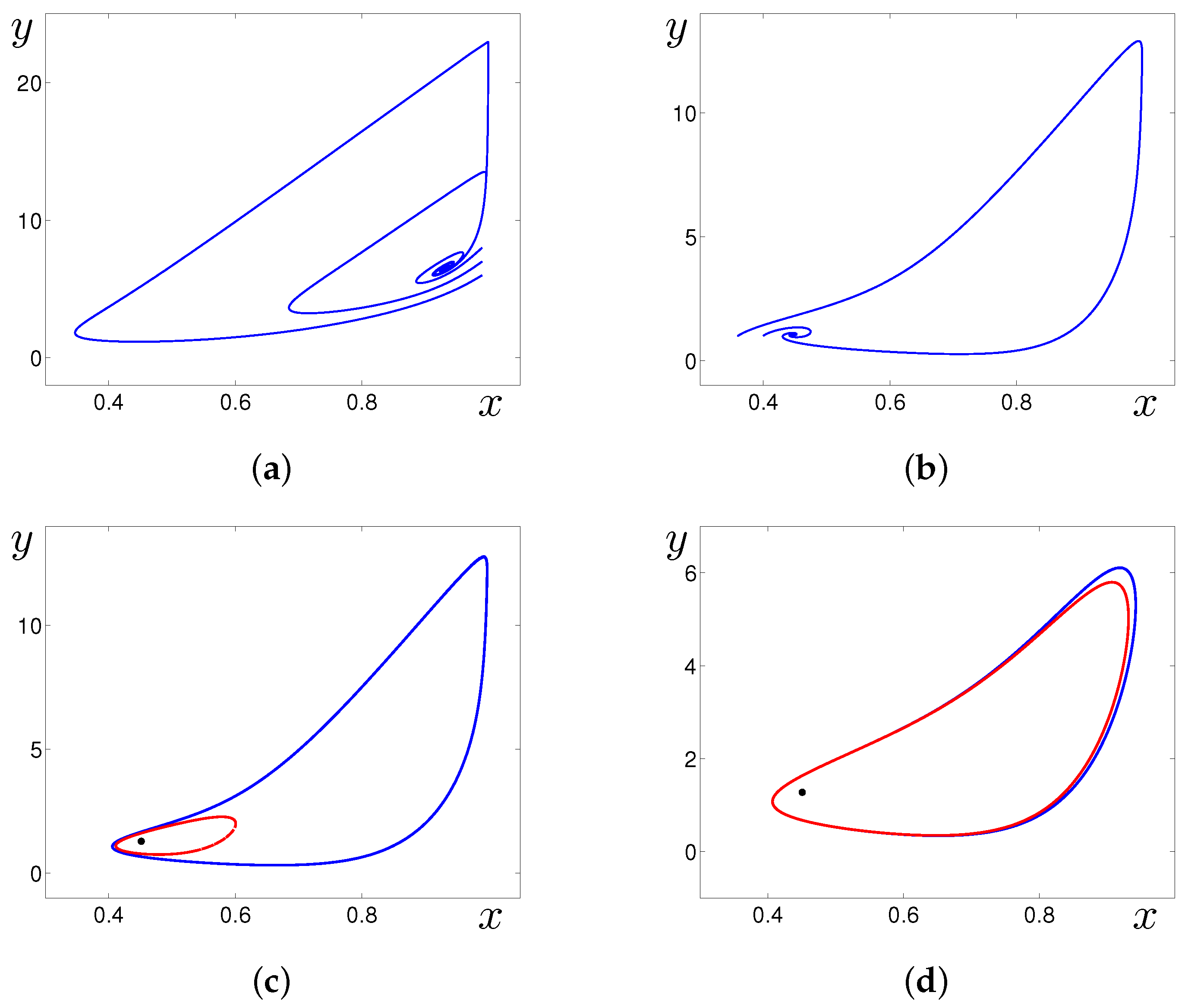
In Figure 2, phase portraits are shown for several values of the parameter D. In Figure 2a,b, we plot phase trajectories starting near the stable equilibrium M. Here, the high non-uniformity of transients should be mentioned. If the deviation of the initial state from the equilibrium is quite small, then the solution quickly approaches the equilibrium. If the deviation exceeds some threshold, the solution at first exhibits a transient large-amplitude loop before converging to the equilibrium.
In Figure 2c,d, the bistability zone is illustrated. Here, basins of the stable equilibrium M (black dot) and stable limit cycle Γ (blue curve) are separated by the orbit of the unstable cycle (red curve).
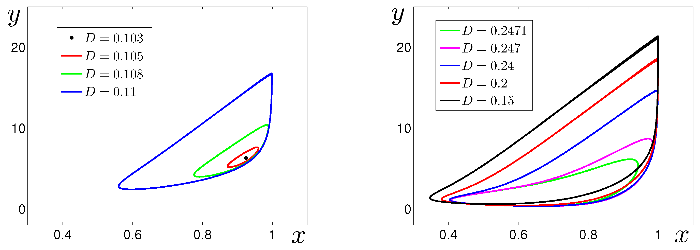
In Figure 3, it is shown how a form and size of limit cycles changes under variations in the parameter D. As the parameter D moves away from the bifurcation points, a size of limit cycle grows, and the shape becomes almost triangular.
So, the deterministic system (1) exhibits both equilibrium and oscillatory kinetic regimes in CSTR. In the following Section, we consider how the system dynamics changes under the random parametric disturbances.

3. Stochastic Model

In the present paper, we analyze impact of random parametric fluctuations in the temperature of the reactor:
x ˙ = ( 1 x ) exp y 1 + β y x D γ y ˙ = ( 1 x ) exp y 1 + β y y S + ε y ξ ( t ) .
Here, in the mathematical modeling of such fluctuations, we use the uncorrelated standard white Gaussian noise ξ ( t ) with parameters E ξ ( t ) = 0 , E ξ ( t ) ξ ( τ ) = δ ( t τ ) . In (2), the scalar parameter ε characterizes the noise intensity.

3.1. Stochastic Excitability

Our study focuses on the stochastic effects in the D-parameter zone D > D 3 adjacent to the saddle-node bifurcation point D 3 = 0.2471004 . In this zone, the equilibrium M is the only attractor of the system (1).
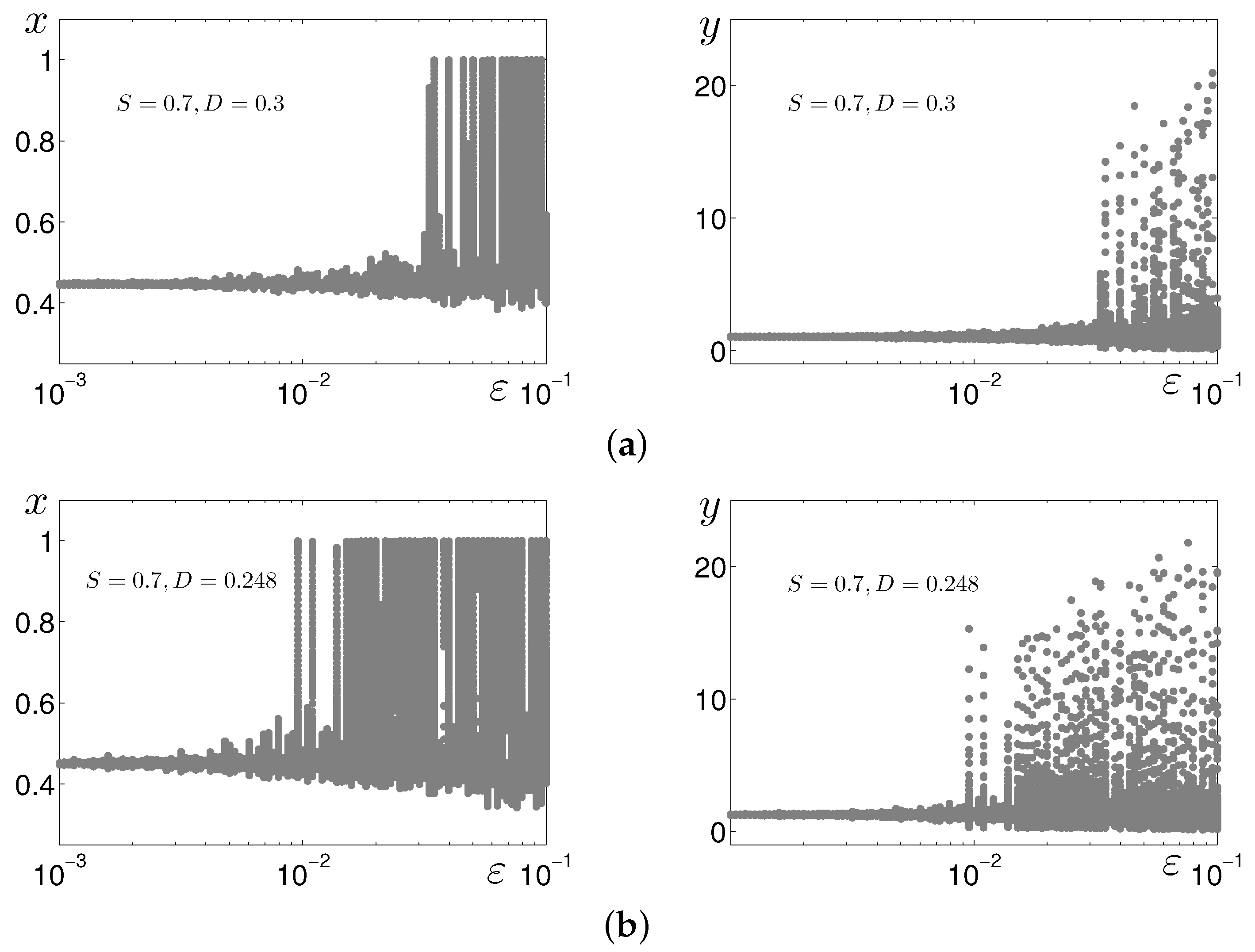
For weak noise, random solutions of the system (2) starting at the equilibrium M are located close to M, and corresponding time series exhibit small-amplitude stochastic oscillations. Under increasing noise intensity, the dispersion of random states around M naturally grows. However, in this growth, a sharp jump is observed: the stochastic system (2) begins to generate large-amplitude spike oscillations.
Such drastic changes in the system (2) dynamics are illustrated in Figure 4, where the x- and y-coordinates of random states are plotted versus the noise intensity ε for two values of the parameter D. These coordinates of random solutions of the system (2) in Poincaré sections with the time step T = 0.01 are plotted by dots. Here, it is clearly seen how small-amplitude oscillations transform into large-amplitude oscillations under increasing noise. This behavior is typical for so-called excitable systems [22]. It should be emphasized that the threshold noise intensity ε * corresponding to such stochastic excitement essentially depends on D: For D = 0.248 (see Figure 4b), the value ε * is smaller than for D = 0.3 (see Figure 4a).
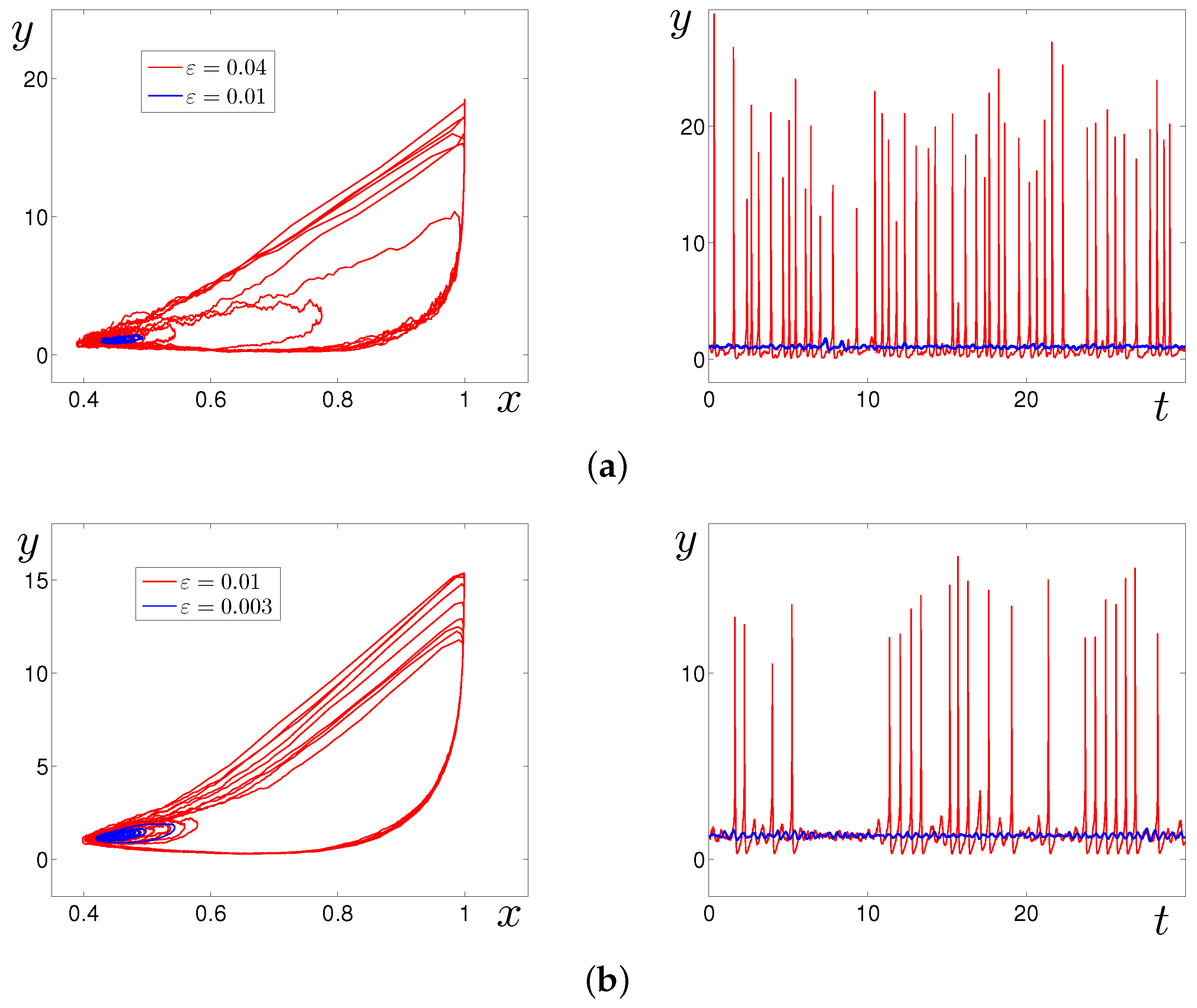
In Figure 5, additional details of the stochastic excitement are shown. It can be seen in the phase trajectories and time series that even with a small change in the noise intensity, small-amplitude stochastic fluctuations transform into mixed-mode ones with alternating noisy oscillations near the equilibrium and large-amplitude spikes. Note that the form of the phase trajectories of generated stochastic oscillations is close to the “triangle” form of the deterministic cycles shown in Figure 3.
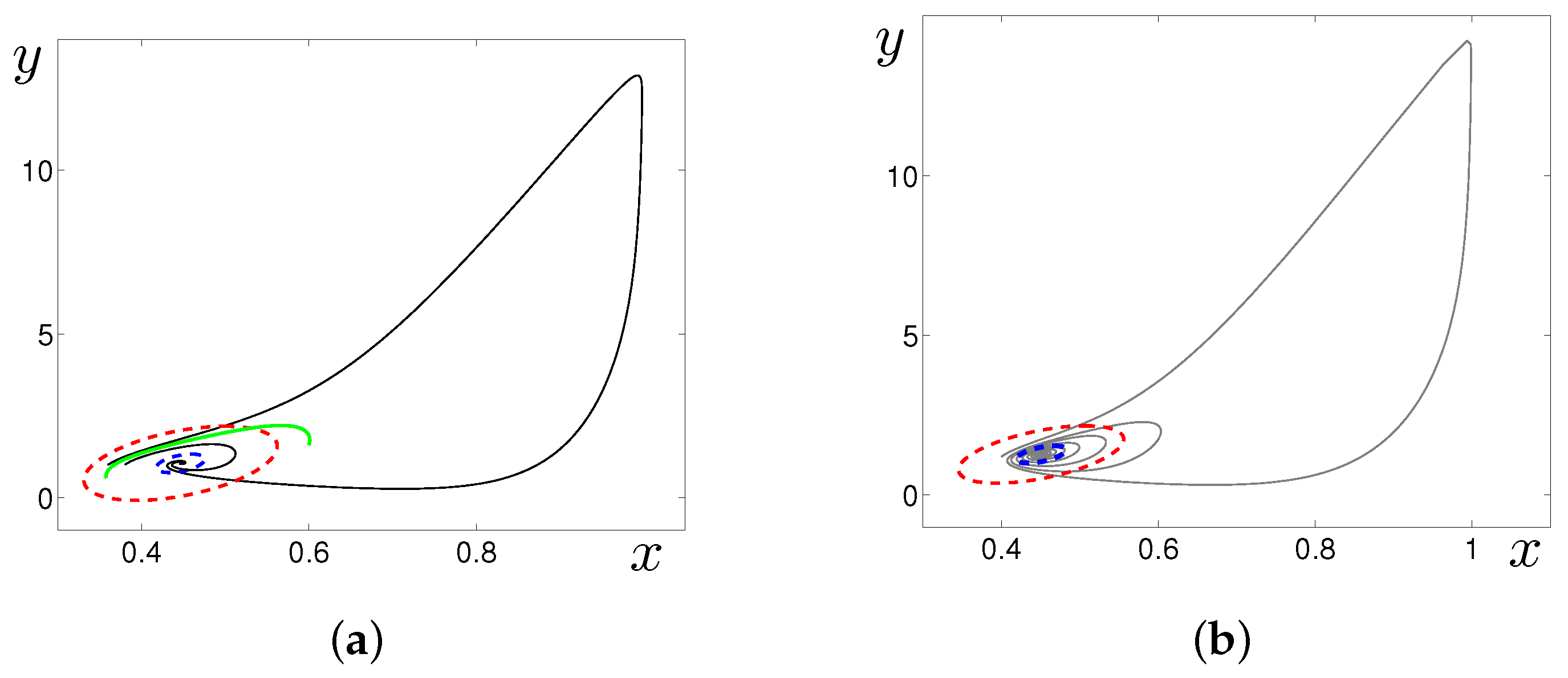
Consider how a mechanism of the noise-induced excitement relates to the peculiarities of the phase portraits of the deterministic system (1). In Figure 6a, one can see two phase trajectories (black) of the deterministic system (1) with D = 0.3 . These trajectories start rather close to the stable equilibrium M. One of the trajectories converges to M at once, whereas the other trajectory first moves away from M and starts approaching it only after passing through a large-amplitude loop. The first trajectory presents the subcritical regime, and the second trajectory corresponds to the supercritical regime. Such a dichotomy is typical for excitable systems.
In the phase plane, the sub- and supercritical zones are separated by a special curve (“pseudo-separatrix”). The “pseudo-separatrix” can be defined as a locally repelling fragment of some deterministic phase trajectory. In Figure 6a, such “pseudo-separatrix” is shown for D = 0.3 by green color. For weak noise, random trajectories do not cross the “pseudo-separatrix” and totally belong to the subcritical zone. As a result, the stochastic system exhibits small-amplitude fluctuations. Under increasing noise, random trajectories cross this “pseudo-separatrix”, fall into the supercritical zone, and exhibit spiking loops. So, to analyse the noise-induced generation of spiking oscillations, one has to take into account the location of the “pseudo-separatrix” and the arrangement of random states around M.
An exhaustive description of probability distributions is given by the Fokker–Planck–Kolmogorov equation. Due to technical difficulties that arise even in the two-dimensional case, various kinds of approximations are usually used [29]. When studying stochastic effects in the ZS model, we apply the constructive approximation method based on the stochastic sensitivity technique. Mathematical details of this approach are presented in the next section.

3.2. Stochastic Sensitivity and Confidence Domains

In this paper, for the description of probabilistic distributions, we will use confidence domains based on the quasipotential method [28] and the stochastic sensitivity function technique [31,32,38].
Let us shortly discuss our approach. Consider the following general nonlinear stochastic system:
x ˙ = f ( x ) + ε g ( x ) ξ ( t ) ,
where x is an n-vector, f ( x ) is an n-vector function, g ( x ) is an n × m -matrix function, ξ ( t ) is standard m-dimensional white Gaussian noise, and ε is a scalar parameter of noise intensity.
Suppose that the deterministic system (3) (with ε = 0 therein) has a stable equilibrium x ¯ . For small noise, an approximation of the density ρ ( x , ε ) of the stationary probabilistic distribution of random states around the equilibrium x ¯ is given by the following formula:
ρ ( x , ε ) K · exp v ( x ) ε 2 .
Here, the quasipotential v ( x ) is a solution of the Hamilton–Jacobi equation:
f ( x ) , v x + 1 2 v x , g ( x ) g ( x ) v x = 0
with the condition v | x ¯ = 0 , v | x x ¯ > 0 .
In a small neighborhood of the deterministic equilibrium x ¯ , one can use a quadratic approximation [39] of the quasipotential and construct an asymptotics of the stationary probabilistic distribution in the Gaussian form:
ρ ( x , ε ) K · exp ( x x ¯ , W 1 ( x x ¯ ) ) 2 ε 2 .
Here, the stochastic sensitivity matrix W is a unique solution of the matrix Lyapunov equation:
F W + W F = G , F = f x ( x ¯ ) , G = g ( x ¯ ) g ( x ¯ ) .
For the two-dimensional Zeldovich–Semenov model (2) with the equilibrium M ( x ¯ , y ¯ ) , we have:
F = e ( y ¯ ) 1 D ( 1 x ¯ ) ( 1 + β y ¯ ) 2 e ( y ¯ ) 1 γ e ( y ¯ ) ( 1 x ¯ ) γ ( 1 + β y ¯ ) 2 e ( y ¯ ) 1 γ S , e ( y ) = exp y 1 + β y , G = 0 0 0 y ¯ 2 γ 2 .
Using the stochastic sensitivity matrix W, one can construct the confidence ellipse:
z 1 2 λ 1 + z 2 2 λ 2 = 2 ε 2 ln ( 1 P ) .
Here, λ 1 and λ 2 are eigenvalues of the stochastic sensitivity matrix W; z 1 and z 2 are coordinates of this ellipse in the basis of eigenvectors v 1 and v 2 , respectively, with the equilibrium M as the origin; ε is the noise intensity; and P is the fiducial probability.
Now, consider how confidence ellipses work in the analysis of noise-induced excitement in the stochastic system (2). In Figure 6a, for D = 0.3 , confidence ellipses are plotted for ε = 0.01 (blue) and ε = 0.04 (red). As can be seen, the smaller ellipse corresponding to ε = 0.01 entirely belongs to the subthreshold zone (below green “pseudoseparatrix”). Such arrangement signals about the location of random states in a small vicinity of the equilibrium M, and therefore, about small-amplitude fluctuations near M.
For ε = 0.04 , the ellipse intersects the “pseudoseparatrix” and partially occupies the superthreshold zone. This means that random solutions can go to the large-amplitude excursions, so, the noise-induced excitement occurs. This prediction agrees well with the results of the direct numerical simulation presented in Figure 4a and Figure 5a.
In Figure 6b, we show how the confidence ellipses method predicts noise-induced excitement for D = 0.248 . Indeed, for ε = 0.003 , the confidence ellipse (blue) lies in the subthreshold zone, whereas the larger ellipse with ε = 0.01 exits to the superthreshold zone. As can be seen, in this case, such an arrangement of confidence ellipses gives a good prognosis of the noise-induced excitement (compare with Figure 4b and Figure 5b).
To summarize, the closer parameter D to the bifurcation point D 3 , the smaller noise intensity is needed for the onset of the stochastic excitement.

3.3. Stochastic P-Bifurcations

Consider how the noise-induced excitement causes qualitative changes in the probability density forms. Peaks of the probability density localize zones of the phase space where random solutions reside more probably. Changes in the location and especially in the number of peaks characterize abrupt transformations of the system dynamics. Changes in the modality of the probability density function are called the stochastic P-bifurcations [11].
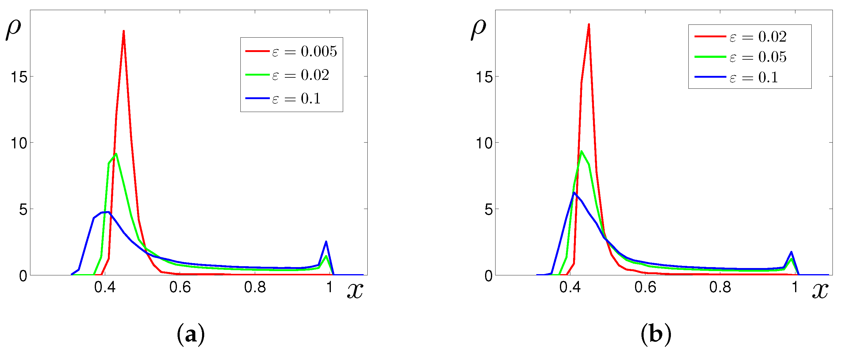
In Figure 7, we show plots of the stationary probability density function ρ ( x ) of the system (2) solutions for two values of D and several ε . In Figure 7a, for D = 0.248 , one can see that with increasing noise, the form of the probability density function ρ ( x ) transforms from one peak to two peaks. The one-peak form (red) for ε = 0.005 reflects the subcritical regime with small-amplitude stochastic oscillations near the equilibrium M. With enhancing noise, because of stochastic excitement, this peak of ρ ( x ) becomes lower and wider, and the second peak appears near x = 1 . Such change in the modality of the function ρ ( x ) can be interpreted as the stochastic P-bifurcation.
In Figure 7b, the stochastic P-bifurcation is shown for D = 0.3 . As can be seen, here, the P-bifurcation occurs for larger noise intensity. This fact agrees with the prognosis given by confidence ellipses in Figure 6.
Now, after studying the changes in the amplitude characteristics of the noise-induced oscillations, let us proceed to the analysis of their frequency properties in the following section.

3.4. Frequency Characteristics of Stochastic Oscillations

Consider how, with increasing noise, the frequency of spiking oscillations changes in the regime of stochastic excitement. In Figure 8, we show time series of the system (2) with D = 0.248 for different values of the noise intensity ε . As can be seen, for weak noise, these spikes are rare, and time intervals τ between successive spikes (interspike intervals, ISI) are quite large.
With the enhancing noise, the frequency of the spikes grows. For the quantitative description of frequency changes, we carry out the statistical analysis of interspike intervals. Here, we use their mean values m = E τ and coefficient of variation C V . In Figure 9a, plots of the function m ( ε ) are shown for three values of the parameter D. These plots allow one to trace how the frequency of spikes depends on the parameters D and ε . Indeed, for weak noise, mean values m are large. The ε -interval where the plot m ( ε ) sharply falls down localizes the threshold noise intensity corresponding to the onset of excitement. Here, it is clearly seen that the larger D is, the greater this threshold noise intensity. For all D, as ε increases, the mean values of ISI decrease, stabilize, and become almost the same.
The dispersion of ISI changes in a more complex way. In Figure 9b, a plot of C V ( ε ) is shown for D = 0.248 . As can be seen, the function C V ( ε ) is not monotonous and has a definite minimum. This means that in some ε -interval, noise-induced spiking oscillations become more coherent. Such a phenomenon is classified as coherence resonance [19,40,41]. For D = 0.248 , the coherence resonance occurs for ε = 0.05 .

4. Discussion and Conclusions

The present paper was devoted to the problem of mathematical modeling and analysis of stochastic generation of mixed-mode oscillations in thermochemical processes. Such complex oscillations take place in real thermochemical reactors [10]. The study of the causes of such oscillations is an important mathematical problem. In our paper, we used the Zeldovich–Semenov model of the continuous stirred tank reactor with random disturbances in temperature. The parametric analysis of the attractors and bifurcations in initial unforced deterministic model was carried out. We revealed a stochastic phenomenon of the noise-induced transformation of the equilibrium regime into mixed-mode oscillatory regime. An underlying mechanism of a such transformation was clarified by the detailed analysis of peculiarities of phase portraits and identifying sub- and superthreshold zones in the phase plane. In the parametric analysis of stochastic excitement, the analytical method of confidence domains was effectively used. Analyzing a mutual arrangement of the confidence ellipses and separatrices, we estimated the critical intensity of the noise that causes the excitation. Amplitude and frequency properties of spiking oscillations induced by multiplicative noise were investigated, and phenomena of stochastic P-bifurcations and coherence resonance were discovered and discussed.

Author Contributions

Conceptualization, I.B. and L.R.; methodology, L.R.; software, I.B.; writing, I.B. and L.R. All authors have read and agreed to the published version of the manuscript.

Funding

The work was supported by RFBR (20-01-00165).

Institutional Review Board Statement

Not applicable.

Informed Consent Statement

Not applicable.

Data Availability Statement

The data presented in this study are available on request from the corresponding author.

Conflicts of Interest

The authors declare no conflict of interest.

References

  1. Uppal, A.; Ray, W.H.; Poore, A.B. The classification of the dynamic behavior of continuous stirred tank reactors—Influence of reactor resident time. Chem. Eng. Sci. 1976, 31, 205–214. [Google Scholar] [CrossRef]
  2. Sheplev, V.S.; Treskov, S.A.; Volokitin, E.P. Dynamics of a stirred tank reactor with first-order reaction. Chem. Eng. Sci. 1998, 53, 3719–3728. [Google Scholar] [CrossRef]
  3. Kawczyński, A.L.; Nowakowski, B. Master equation simulations of a model of a thermochemical system. Phys. Rev. E 2003, 68, 036218. [Google Scholar] [CrossRef] [PubMed]
  4. Semenov, N.N. Theories of combustion processes. Z. Phys. Chem. 1928, 48, 571–582. [Google Scholar]
  5. Zeldovich, J.B.; Zysin, J.A. On the theory of heat stress. Exothermic reaction in the jet. Zhurnal Tekhnicheskoi Fiz. 1941, 11, 501–508. [Google Scholar]
  6. Frank-Kamenetskii, D.A. Diffusion and Heat Exchange in Chemical Kinetics; Princeton University Press: Princeton, NJ, USA, 1955. [Google Scholar]
  7. Vaganov, D.A.; Samoilenko, N.G.; Abramov, V.G. Periodic regimes of continuous stirred tank reactors. Chem. Eng. Sci. 1978, 33, 1131–1140. [Google Scholar] [CrossRef]
  8. Bykov, V.I.; Serafimov, L.A.; Tsybenova, S.B. Emergency starting regimes of a continuous stirred tank reactor. Theor. Found. Chem. Eng. 2015, 49, 361–369. [Google Scholar] [CrossRef]
  9. Bykov, V.I.; Tsybenova, S.B. Parametric analysis of the simplest model of the theory of thermal explosion–the Zel’dovich–Semenov model. Combust. Explos. Shock Waves 2001, 37, 523–534. [Google Scholar] [CrossRef]
  10. Bykov, V.I.; Tsybenova, S.B.; Yablonsky, G. Chemical Complexity via Simple Models; De Gruyter: Berlin, Germany, 2018. [Google Scholar]
  11. Arnold, L. Random Dynamical Systems; Springer: Berlin, Germany, 1998; p. 600. [Google Scholar]
  12. Bashkirtseva, I.; Ryazanova, T.; Ryashko, L. Stochastic bifurcations caused by multiplicative noise in systems with hard excitement of auto-oscillations. Phys. Rev. E 2015, 92, 042908. [Google Scholar] [CrossRef]
  13. Simpson, S.H.; Arita, Y.; Dholakia, K.; Zemánek, P. Stochastic Hopf bifurcations in vacuum optical tweezers. Phys. Rev. A 2021, 104, 043518. [Google Scholar] [CrossRef]
  14. Horsthemke, W.; Lefever, R. Noise-Induced Transitions; Springer: Berlin, Germany, 1984; p. 338. [Google Scholar]
  15. Bashkirtseva, I.; Chen, G.; Ryashko, L. Analysis of noise-induced transitions from regular to chaotic oscillations in the Chen system. Chaos 2012, 22, 033104. [Google Scholar] [CrossRef] [PubMed] [Green Version]
  16. Coti Zelati, M.; Hairer, M. A noise-induced transition in the Lorenz system. Commun. Math. Phys. 2021, 383, 2243–2274. [Google Scholar] [CrossRef]
  17. Anishchenko, V.S.; Astakhov, V.V.; Neiman, A.B.; Vadivasova, T.E.; Schimansky-Geier, L. Nonlinear Dynamics of Chaotic and Stochastic Systems. Tutorial and Modern Development; Springer: Berlin/Heidelberg, Germany, 2007; p. 535. [Google Scholar]
  18. McDonnell, M.D.; Stocks, N.G.; Pearce, C.E.M.; Abbott, D. Stochastic Resonance: From Suprathreshold Stochastic Resonance to Stochastic Signal Quantization; Cambridge University Press: Cambridge, UK, 2008; p. 446. [Google Scholar]
  19. Pikovsky, A.S.; Kurths, J. Coherence resonance in a noise-driven excitable system. Phys. Rev. Lett. 1997, 78, 775–778. [Google Scholar] [CrossRef] [Green Version]
  20. Bashkirtseva, I.; Ryashko, L. How additive noise generates a phantom attractor in a model with cubic nonlinearity. Phys. Lett. A 2016, 380, 3359–3365. [Google Scholar] [CrossRef]
  21. Ryashko, L.; Alexandrov, D.; Bashkirtseva, I. Analysis of stochastic generation and shifts of phantom attractors in a climate–vegetation dynamical model. Mathematics 2021, 9, 1329. [Google Scholar] [CrossRef]
  22. Lindner, B.; Garcia-Ojalvo, J.; Neiman, A.; Schimansky-Geier, L. Effects of noise in excitable systems. Phys. Rep. 2004, 392, 321–424. [Google Scholar] [CrossRef]
  23. Orcioni, S.; Paffi, A.; Apollonio, F.; Liberti, M. Revealing spectrum features of stochastic neuron spike trains. Mathematics 2020, 8, 1011. [Google Scholar] [CrossRef]
  24. Lima Dias Pinto, I.; Copelli, M. Oscillations and collective excitability in a model of stochastic neurons under excitatory and inhibitory coupling. Phys. Rev. E 2019, 100, 062416. [Google Scholar] [CrossRef]
  25. Gao, J.B.; Hwang, S.K.; Liu, J.M. When can noise induce chaos? Phys. Rev. Lett. 1999, 82, 1132–1135. [Google Scholar] [CrossRef] [Green Version]
  26. Lai, Y.C.; Tel, T. Transient Chaos. Complex Dynamics on Finite Time Scales; Springer: New York, NY, USA, 2011; p. 502. [Google Scholar]
  27. Bashkirtseva, I.; Ryashko, L.; Slepukhina, E. Noise-induced oscillation bistability and transition to chaos in FitzHugh-Nagumo model. Fluct. Noise Lett. 2014, 13, 1450004. [Google Scholar] [CrossRef]
  28. Freidlin, M.I.; Wentzell, A.D. Random Perturbations of Dynamical Systems; Springer: New York, NY, USA; Berlin, Germany, 1984. [Google Scholar]
  29. Gardiner, C.W. Handbook of Stochastic Methods for Physics, Chemistry and the Natural Sciences; Springer: Berlin, Germany, 1983. [Google Scholar]
  30. Dembo, M.; Zeitouni, O. Large Deviations Techniques and Applications; Jones and Bartlett Publishers: Boston, MA, USA, 1995; p. 396. [Google Scholar]
  31. Bashkirtseva, I.; Ryashko, L. Sensitivity analysis of stochastically forced Lorenz model cycles under period doubling bifurcations. Dyn. Syst. Appl. 2002, 11, 293–310. [Google Scholar]
  32. Bashkirtseva, I.; Chen, G.; Ryashko, L. Analysis of stochastic cycles in the Chen system. Int. J. Bifurc. Chaos 2010, 20, 1439–1450. [Google Scholar] [CrossRef]
  33. Danylenko, V.; Skurativskyi, S. Stationary and periodic regimes in relaxing media with fluctuations. Eur. Phys. J. B 2014, 87, 218. [Google Scholar] [CrossRef]
  34. Sun, Y.; Hong, L.; Jiang, J. Stochastic sensitivity analysis of nonautonomous nonlinear systems subjected to Poisson white noise. Chaos Solitons Fractals 2017, 104, 508–515. [Google Scholar] [CrossRef]
  35. Xu, C.; Yuan, S.; Zhang, T. Confidence domain in the stochastic competition chemostat model with feedback control. Appl. Math. J. Chin. Univ. 2018, 33, 379–389. [Google Scholar] [CrossRef]
  36. Xu, C.; Yuan, S.; Zhang, T. Sensitivity analysis and feedback control of noise-induced extinction for competition chemostat model with mutualism. Phys. A Stat. Mech. Its Appl. 2018, 505, 891–902. [Google Scholar] [CrossRef]
  37. Das, P.; Mukherjee, S.; Das, P.; Banerjee, S. Characterizing chaos and multifractality in noise-assisted tumor-immune interplay. Nonlinear Dyn. 2020, 101, 675–685. [Google Scholar] [CrossRef]
  38. Alexandrov, D.V.; Bashkirtseva, I.A.; Crucifix, M.; Ryashko, L.B. Nonlinear climate dynamics: From deterministic behaviour to stochastic excitability and chaos. Phys. Rep. 2021, 902, 1–60. [Google Scholar] [CrossRef]
  39. Mil’shtein, G.; Ryashko, L. A first approximation of the quasipotential in problems of the stability of systems with random non-degenerate perturbations. J. Appl. Math. Mech. 1995, 59, 47–56. [Google Scholar] [CrossRef]
  40. García-Vellisca, M.A.; Pisarchik, A.N.; Jaimes-Reátegui, R. Experimental evidence of deterministic coherence resonance in coupled chaotic systems with frequency mismatch. Phys. Rev. E 2016, 94, 012218. [Google Scholar] [CrossRef]
  41. Jaimes-Reátegui, R.; García-López, J.; Gallegos, A.; Huerta Cuellar, G.; Chholak, P.; Pisarchik, A. Deterministic coherence and anti-coherence resonances in networks of chaotic oscillators with frequency mismatch. Chaos Solitons Fractals 2021, 152, 111424. [Google Scholar] [CrossRef]
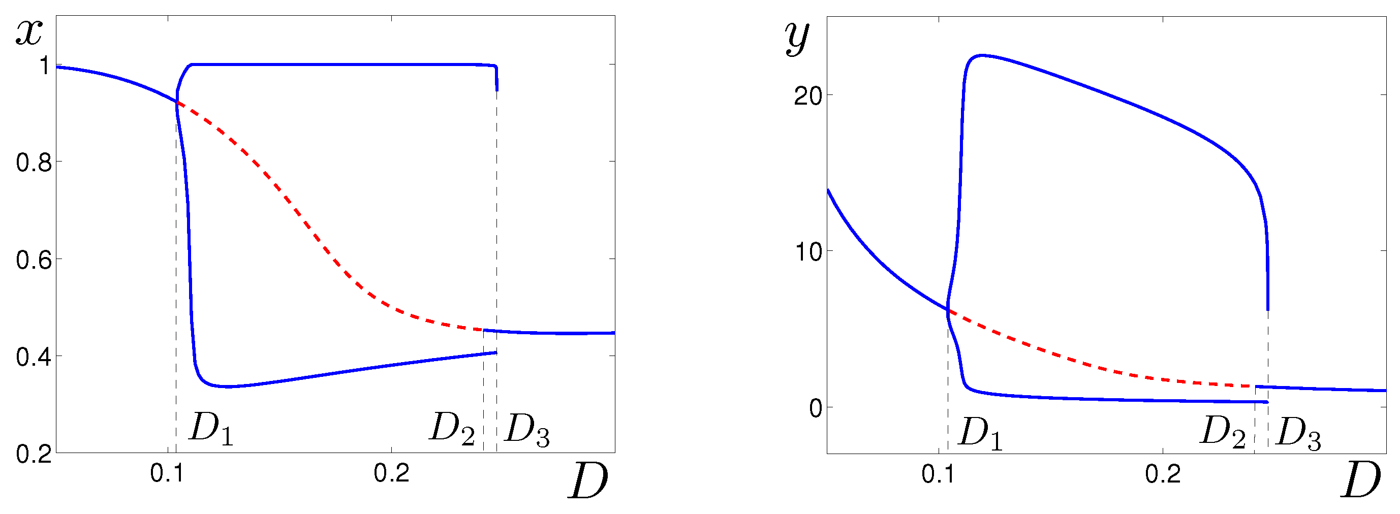
Figure 1. Bifurcation diagram for γ = 0.03 , S = 0.7 .
Mathematics 10 00960 g001
Figure 2. Phase portraits of the system (1) for (a) D = 0.1 , (b) D = 0.3 , (c) D = 0.245 , (d) D = 0.2471 .
Mathematics 10 00960 g002
Figure 3. Limit cycles of the system (1).
Mathematics 10 00960 g003
Figure 4. Random states of the system (2) for (a) D = 0.3 , (b) D = 0.248 .
Mathematics 10 00960 g004
Figure 5. Stochastic trajectories and time series of the system (2): (a) for D = 0.3 and noise intensities ε = 0.01 (blue), ε = 0.04 (red); (b) for D = 0.248 and noise intensities ε = 0.003 (blue), ε = 0.01 (red).
Mathematics 10 00960 g005
Figure 6. Confidence ellipses around the equilibrium M: (a) for D = 0.3 and noise intensities ε = 0.01 (blue), ε = 0.04 (red); (b) for D = 0.248 and noise intensities ε = 0.003 (blue), ε = 0.01 (red). Here, fiducial probability P = 0.99 .
Mathematics 10 00960 g006
Figure 7. Stochastic P-bifurcations in the system with (a) for D = 0.248 , (b) for D = 0.3 .
Mathematics 10 00960 g007
Figure 8. Noise-induced spiking oscillations in the system (2) with D = 0.248 for: (a) ε = 0.006 , (b) ε = 0.01 , (c) ε = 0.05 .
Mathematics 10 00960 g008
Figure 9. Frequency characteristics of oscillations in the stochastic system: (a) mean values m of interspike intervals, (b) coefficient of variation for D = 0.248 .
Mathematics 10 00960 g009
Publisher’s Note: MDPI stays neutral with regard to jurisdictional claims in published maps and institutional affiliations.