Abstract
Customers’ expectations of timely and accurate delivery and pickup of online purchases pose a new challenge to last-mile delivery. When the goods sent to customers are not received, they must be returned to the warehouse. This situation provides a high additional cost. Parcel locker systems and convenience stores have been launched to solve this problem and serve as pickup and payment stations. This research investigates a new last-mile distribution problem in the augmented system with three service modes: home delivery and pickup, parcel locker delivery and pickup, and home or parcel locker delivery and pickup. Previously, the simultaneous delivery and pickup problem with time windows (SDPPTW) only considered delivery and pickup to customers. The new problem proposed in this research addresses additional locker pickup and delivery options. The proposed problem is called the vehicle routing problem with simultaneous pickup and delivery and parcel lockers (VRPSPDPL). This research formulated a new mathematical model and developed two simulated annealing (SA) algorithms to solve the problem. The goal is to minimize the total traveling cost. Since there are no existing benchmark instances for the problem, we generate new instances based on SDPPTW benchmark instances. The experimental results show that the proposed algorithms are effective and efficient in solving VRPSPDPL.
1. Introduction
Logistics service and delivery accrue the highest cost in the E-Commerce industry and affect online purchases [1]. To respond to the challenges of last-mile delivery problems, companies must seek reliable distribution strategies for multiple dimensions, such as cost-effectiveness, customer satisfaction, delivery option, and sustainability [2]. Parcel lockers have become a potential delivery option, among different methods, to handle the last-mile delivery [3].
The classical delivery method to consumers’ homes requires very high operational costs to serve many orders, especially for business-to-consumer (B2C) service, which is currently increasing [4]. Parcel locker implementation into B2C could save 55–66% of transportation costs, compared to the conventional logistic system [3]. Moreover, since the parcel locker system provides flexibility and efficiency for delivery and picks up products, its integration can improve the service experience and provide a competitive advantage in the logistic system [5].
Many studies have explored and investigated delivery options such as parcel lockers in different aspects. The total profit can be maximized by determining the parcel locker configuration, such as the number of lockers, positions, and sizes [3]. Some researchers have developed a decision-making model to determine parcel locker facilities [6]. Locating parcel lockers could be addressed as optimization problems, such as network problems [3] or delivery options with vehicle routing [7]. Research on parcel lockers in the vehicle routing problem is a challenging and continuously evolving research area as it provides an opportunity to reduce costs [8].
Various approaches have been developed to address the issues associated with parcel lockers, but there is a lack of research on integrating parcel locker with pickup and delivery in logistics. For example, previous studies introduced a vehicle routing problem with simultaneous pickup and delivery and handling cost [9,10] but did not consider parcel lockers. Another research developed a two-echelon vehicle routing problem covering options via bikes or lockers but not simultaneously operated pickup and delivery [11]. Some studies analyzed parcel locker characteristics and travel access but ignored a vehicle’s route to deliver the goods [12].
Earlier, simultaneous delivery and pickup service were carried out with a single stop for each customer to reduce transportation costs and service efforts. The couriers only needed to visit each customer within their time frame. This problem is formally described as the simultaneous delivery and pickup problem with time windows (SDPPTW) [13]. Although existing studies in SDPPTW have provided various benefits [14], the high demand for flexibility and efficiency for pickup and delivery anytime all day (24 h) posed a new challenge. Moreover, the actual condition requires more than a single mode to deliver and pick up products. The customer can choose several delivery modes to receive or return the goods [15]. To fill this gap, the integration of pickup and delivery options is needed.
This study introduces a new logistics problem called the vehicle routing problem with simultaneous pickup and delivery and parcel lockers (VRPSPDPL). The VRPSPDPL considers three types of customers: first, customers who require delivery and pickup at their home location; second, customers who selected parcel lockers to receive and send packages; and third, customers who are willing to accept and deliver packages either at their home locations or at parcel lockers. For the parcel locker system introduced in this research, customers are informed by messaging when the good has arrived at the locker. They need to pick up the packages themselves, not necessarily concerned about staying at home or flexibility in time. VRPSPDPL also considers the parcel locker’s capacity, the time window of each customer, and the vehicle’s capacity. The objective of VRPSPDPL is to minimize traveling costs.
Since previous work has never dealt with VRPSPDPL, we developed a new mathematical programming model for the problem. VRPSPDPL is an NP-hard problem because it is developed from SDPPTW, an NP-hard problem [13]. Therefore, to optimize VRPSPDPL, a metaheuristic is selected because it provides a practical alternative designed to achieve near-optimal solutions for NP-hard problems [16]. Among various metaheuristic methods, we decided to use simulated annealing (SA) since it has shown competitive performance and promising results in many cases [17]. Moreover, the SA algorithm has proven to provide a good result for various types of VRP, e.g., capacitated vehicle routing problem (CVRP) [17], vehicle routing problem with time windows (VRPTW) [18], hybrid vehicle routing problem (hybrid-VRP) [19], time-dependent vehicle routing problem (TD-VRP) [20], green vehicle routing problem (G-VRP) [21], path cover problem with time windows (PCPTW) [22], and VRP with pickup delivery [23].
For computational studies, we generated VRPSPDPL benchmark instances by modifying SDPPTW benchmark instances. These new instances are used to test the VRPSPDPL model and compare the solutions’ output from the Gurobi solver and the proposed SA algorithm. By doing so, we managed to assess the performance of the proposed SA algorithm.
The novel contribution of the paper is two-fold. First, we introduce a new mathematical programming model for VRPSPDPL. This model is expected to be a promising method to solve the problem of last-mile delivery. Second, we developed efficient metaheuristics, i.e., SA with and SA without backtrack (SAwb), to solve the model.
This paper consists of six sections. The following section presents a review of the relevant literature and research gap. In Section 3, we describe the definitions, assumptions, and mathematical formulations for VRPSPDPL. The solution representation, initial solution, and proposed simulated annealing algorithms are described in Section 4. Section 5 presents a numerical experiment to demonstrate the performance of the proposed model and algorithms. Finally, notable findings and insights from this research are summarized in Section 6.
2. Literature Review
The vehicle routing problem with simultaneous pickup and delivery and parcel lockers is developed initially from the vehicle routing problem with simultaneous pickup and delivery and time windows (VRPSPDTW) by integrating the problem with parcel lockers. Angelelli and Mansini [24] introduced VRPSPDTW and proposed a branch-and-cut-and-price algorithm to solve it. The VRPSPDTW is developed to reduce the service effort and interference of the customer by performing simultaneous delivery and pick-up services with a single stop for each customer. By considering time windows, the vehicle has to wait if it arrived before the time window. The VRPSPDTW is also known as simultaneous delivery and pickup problems with time windows (SDPPTW) [13].
The VRPSPDTW has been widely applied to logistics systems and various industries, such as fresh food, soft drink distribution, and foundry [13]. As a vehicle routing problem with simultaneous pickup and delivery (VRPSPD) variant, the VRPSPDTW has been extensively studied with respect to its practical importance for distribution companies and its benefits. Mingyong and Erbao [25] developed a differential evolutionary algorithm for VRPSPDTW and introduced a technical penalty to handle the infeasible solution. Fan [26] used a classical tabu search to maximize customer satisfaction and minimize the total cost for VRPSPDTW. Wang and Chen [13] developed a genetic algorithm based on co-evolution and modified the Solomon [27] benchmark instances into 10, 25, 50, and 100 customer instances. They compared the proposed method with CPLEX and obtained better solutions for medium- and large-size instances with less computational time. Liu et al. [14] implemented VRPSPDTW for home healthcare logistics and proposed a hybrid genetic algorithm and a tabu search heuristic. The problem has four types of demands: deliveries from hospital to patients, deliveries from depot to patients, pickup from patient to the laboratory, or patients to the depot. In general, the proposed method of Liu [14], i.e., tabu search and genetic algorithm, provide good solutions in a reasonable time. Later, Liu et al. [28] proposed a memetic algorithm with efficient local search and extended neighborhood to solve new benchmark instances derived from real-world application of the JD logistics. Thus, it is indicated that research in this area is constantly evolving.
As aforementioned, research in VRPSPDTW is continuously growing and provides various benefits. However, the logistic system requires more flexible service for customers and companies must have competitive advantages. Therefore, a parcel locker was introduced to provide more flexibility, security, and efficiency than the classical delivery system [3]. By implementing parcel locker as a component of delivery option, customers can collect or send their shipments at lockers at a flexible time (24 h), primarily in public areas such as convenience stores, transportation stations, gas stations, or specific places intended for parcel locker. Besides, the company also benefits from reducing transportation costs by reducing the pickup delivery point of the shipment.
The integration of parcel lockers in VRP was first investigated by Zhou et al. [7] by introducing a multi-depot, two-echelon vehicle routing problem with delivery options for last mile distribution (MD–TEVRP–DO). In this problem, customers can be divided into three types of customers, i.e., home delivery customers, selected location delivery customers, and home or selected location delivery customers. A hybrid multi-population genetic algorithm was proposed to solve the problem. However, the model did not consider the time window and only operated delivery to serve customers.
Sitek et al. [29] introduced a capacitated vehicle routing problem with pickup and alternative delivery (CVRPPAD) to minimize the travel distance. They also considered an alternative delivery location in parcel locker stations and introduced time windows related to delivery time. The model was implemented in mathematical programming, logic programming, and a hybrid heuristic environment. Although the authors considered parcel locker and time windows in the model, they did not conduct simultaneous pickup and delivery operations.
Redi et al. [30] introduced a two-echelon vehicle routing problem with locker facilities (2EVRP-LF). The objective was to minimize the cost of transportation, facilities’ cost, and compensation cost. A simulated annealing algorithm was proposed to solve the problem. In this problem, the intermediate facilities are considered locker facilities. However, the model does not operate pickup and delivery simultaneously to the customer and ignores the time windows.
The motivation of this study was to fill the gap and compensate for the drawback of VRPSPDTW by Wang and Chen [13] by investigating parcel locker and delivery options as mentioned by Zhou et al. [7]. According to the available literature, these two major problems, i.e., VRPSPD and parcel locker, worked independently. Even the survey paper related to these studies discussed slightly an integrated problem of VRPSPD and parcel locker. For example, Koç et al. [31] provided an overview of existing work on the VRPSPD but did not discuss the integration of the VRPSPD with parcel lockers. On another side, Rohmer et al. [32] reviewed the parcel locker study in last-mile distribution and provided research opportunities to investigate the vehicle routing problem with parcel lockers. Although they mentioned several implementations of VRP and parcel lockers in the survey paper, there is no study that has integrated VRPSPDTW and parcel lockers.
The VRPSPDPL belongs to NP-hard problems since it was developed from VRPSPDTW, which is an NP-hard problem [33]. Researchers have used various methods to tackle the problem of VRPSPDTW. A classical approach, such as k-trees and the branch-and-bound method, was proposed to solve the problem [34]. Due to its complexity, only limited, exact methods based on a mathematical programming formulation were proposed. Nevertheless, the exact approach has been limited to small- and medium-size instances due to the high computational time [19]. Thus, heuristics have been proposed as remedies to this issue [33]. However, the heuristic approach has the possibility of being trapped in the local optimum solution. Therefore, the metaheuristic approach is widely adopted to overcome this issue.
This research proposes a simulated annealing (SA) heuristic for VRPSPDPL based on a popular simulated annealing heuristic. Since it was introduced by Metropolis et al. in 1953, SA has been successfully applied to various highly complicated combinatorial optimization problems and a wide variety of real case problems. Several implementations of SA, logistic resource planning [35], job rotation scheduling problem [36], pickup and delivery problem [23], and many more, indicate a competitive performance of this approach. Moreover, especially in VRP and its variants, SA is widely used and can provide good results [18,22].
The principle of SA, following the analogy to the physical annealing process in metals, made the SA algorithm capable of escaping local minima, easy implementation, and relatively fast to achieve convergence [37]. The SA algorithm refers to the concept of local search, which begins by generating an initial solution at random. The temperature is initialized, then lowered slowly, following a cooling schedule to achieve minimum energy. While the temperature decreases, the objective function is calculated and a new solution selected from the neighborhood of the current solution. By comparing each solution, the best solution is obtained until the iteration process ends. One of the advantages of SA is its ability to continuously evaluate worse solutions during the iteration process to escape the local optimum.
The standard SA has three variants and improvements [37]. These variants can be divided based on how the method is applied to improve the output quality of SA. The first is a variant based on the cooling schedule. To obtain a global minimum, researchers improve the SA by determining an efficient cooling schedule and the number of iterations at each temperature [38]. Second, a variant is based on neighborhood selection. SA performance usually depends on the initial solution and the neighborhood search. Therefore, the second variant mainly exploits the searching area of the solution and generates a good initial solution. Some researchers combine/hybridize the SA with another algorithm such as genetic algorithm-SA [39], harmony search algorithm-SA [40], and particle swarm optimization-SA [41]. Third, a variant is based on the learning mechanism. The learning mechanism mainly focuses on increasing the speed of SA, such as fast simulated annealing, very fast simulated re-annealing, adaptive-SA, and chaotic-SA [37]. In the development of SA, there are vast opportunities and modifications; thus, the implementation of SA continues to grow.
3. Mathematical Programming Model
VRPSPDPL is an extension of SDPPTW. The main characteristic of VRPSPDPL that differentiates it from SDPPTW is that it considers three types of customers. Type 1 customers are those who can only be served by vehicles at home. For each type 1 customer, a vehicle must be dispatched to the customer’s home to make the delivery or collect the returned product. SDPPTW only considers this type of customer. The type 2 customers are served by parcel lockers. They receive and return their parcels by themselves at parcel lockers. The type 3 customers can be served by vehicles or parcel lockers. They can accept home delivery and pick up and go to parcel lockers to pick up or drop off their parcels. Each type 3 customer has a specific time interval for receiving delivery and pick up services at home. Figure 1 illustrates the VRPSPDPL network to serve three types of customers.
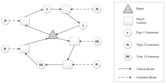
Figure 1.
An illustration of the VRPSPDPL Network.
In this study, all vehicles depart from the depot and return after visiting parcel lockers and serving all customers. Before planning the route, the company knows the current demands for parcel lockers. The demands are generated from the previous service day. After planning the route, subsequently raised demands for parcel lockers are considered on the following service day. All the goods of delivery customers are from the depot and all the products of pickup customers are returned to the depot and not directly delivered to the customers.
In VRPSPDPL, we assume that each vehicle departs from the depot and back to the depot. Each vehicle has the same capacity and each parcel locker has the same capacity. Each customer has fixed delivery and pickup demand. Each customer who is served by the vehicle is precisely served once. Each customer requests pickup and delivery demand at the same time. The capacities of each vehicle and parcel locker are known. The locations of the depot, parcel lockers, and customers are also known. Demands of customers must be put into parcel lockers. Customers who are the second or third type can only choose one specific parcel locker. Customers who are the first type must be at home to pick up and deliver the goods successfully. Delivery demands must originate from the depot, while pickup demands must be transported back to the depot. Before the vehicle departs from the depot, the demands for parcel lockers will be delivered on that day. After the vehicle departs from the depot, parcel lockers’ demands are delivered the next day.
The VRPSPDPL model can be represented as a complete directed Graph where is a set of nodes representing customers and depots . A set of customers , where . Set of customers and parcel lockers are denoted as , i.e., . is a set of edges connecting each pair of nodes in . Set of type 1 customer is denoted by , set of type 2 customer is denoted by , and set of type 3 customer is denoted by . The set of parcel lockers is denoted by . Associated with each edge, is a traveling cost and traveling time from node to where . A set of the vehicle is denoted by . Each vehicle has capacity . To differentiate between the amount picked up and delivered by the customer, we symbolize as the delivery amount of the customer and as the pickup amount of customer , . is the set containing all the customers and parcel locker stations. Since the VRPSPDPL considers time windows, and denote the earliest service time and latest service time, respectively, of node . Each node has to represent the service time of node . If customer is allocated to parcel , then ; otherwise , where , . Lastly, we define as an arbitrarily large number. The number of customers serviced by parcel lockers cannot be larger than , where .
The goal of VRPSPDPL is to minimize total traveling costs by determining which routes should be constructed to serve customers and parcel lockers. The decision variables are as follows.
| If vehicle is from node to node , ; otherwise , , , . | |
| If customer is served by the vehicle, ; otherwise , . | |
| If customer is served by parcel locker, ; otherwise , . | |
| Load of vehicle when leaving the depot, . | |
| Load of vehicle after having serviced node , , . | |
| Starting time of vehicle to service node , , . | |
| If customer is served by the parcel locker , ; otherwise , , . | |
| If vehicle services the demands from parcel locker , = 1; otherwise = 0,, . | |
| The value used to avoid subtour, , . |
The mathematical programming model for the problem is as follows:
Subject to:
The objective Function (1) aims to minimize the total traveling cost. Constraint (2) ensures that different types of customers have different service methods. Type 1 customers are those that can only be served by vehicles. Meanwhile, type 2 customers are those who can only be served by parcel lockers. Type 3 customers are those who can be served by vehicles or parcel lockers. Constraint (3) ensures that each vehicle starts from the depot. Constraint (4) ensures that the same vehicle enters and leaves each customer; this guarantees route continuity. Constraints (5) to (8) are related to time windows to ensure that the arrival time and serving time does not violate vehicles’ continuity. Constraint (9) to (15) are vehicle load constraints associated with initial vehicle loads, vehicle loads after serving the first customer, and vehicle loads in route, individually. Constraint (16) is a vehicle capacity constraint, which assures that the number of goods never exceeds a vehicle’s specified capacity. Constraint (17) ensures parcel lockers can serve the number of customers. Constraint (18) specifies that the designated parcel locker can serve customers. Constraints (19) and (20) specify each type of customer. Constraints (21) and (22) ensure if the customer is served by a parcel locker or not. Constraints (23) and (24) are the demand constraint for the parcel locker. This is to assure that the demand for each parcel locker is satisfied by the vehicle. Constraint (25) ensures that there are no routes for the same node. Constraint (26) is used for subtour elimination. Constraints (27) to (32) define all of the decision variables.
4. Simulated Annealing for VRPSPDPL
In this section, the solution representation of the problem, the initial solution, neighborhood moves, and the developed SA algorithm are explained.
SA algorithm operates using the analogy of the cooling or annealing process. The mechanism starts with determining an initial solution to find a (near) global minimum by imitating the slow cooling procedure of the annealing process. A new solution is determined from the predefined neighborhood of the current solution at each iteration. The new solution’s objective function value was calculated and compared with the current best solution for each iteration. By doing so, we could evaluate whether an improvement has been achieved. If the objective function value of the new solution is better than the previous, then the new solution becomes the current solution. However, if a new solution is worse than the previous, the new solution may still be accepted using a calculation determined by the Boltzmann function, . is the difference in objective function values between the current solution and the new solution, is a Boltzmann constant, and is the current temperature. A random value ranging from 0 to 1 is generated. If , then the new neighborhood solution is accepted as a new current solution; otherwise, it is rejected. Through this mechanism, SA can avoid being trapped in the local optimum [35].
4.1. Solution Representation
The solution of the VRPSPDPL consists of a string number of customers, parcel lockers, and depot. It is denoted by one depot , customers , and parcel lockers . To demonstrate the solution representation, we use the example of 25 customers and 2 parcel lockers. As shown in Figure 2, a two-dimensional array describes a solution representation of the VRPSPDPL. The array includes two parts: the first part is the original node of the visiting route and the second part is the ultimately visiting route node. The length of the two parts is the same. The beginning and end of routes are both 0. The first part records a serial number of each node and the actual delivery location of the vehicles is added in the second part.
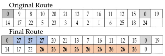
Figure 2.
Solution representation of the VRPSPDPL.
Figure 2 shows the generation of the second part of the solution representation. If the node at the original route is a 0 or type 1 customer, then the relative position node at the final route is 0. The 0 is also used to separate different routes. In this example, there are two routes. The first route services customers 9, 8, 10, 20, 21, 13, 7, 16, 11, 12, and 15, while the second route is for the remaining customers.
For instance, a customer number equals 20 is a type 1 customer. Consequently, the node position at the final route must be 20. If the customer number 14 is a type 2 customer, parcel locker number 26 or 27 must serve this type of customer, so the relative position node at the final route must be 26 or 27. Furthermore, if the customer number 4, referred to as a type 3 customer, then the vehicle or parcel locker may serve this customer—the relative position node at the final route could be 4, 26, or 27. In this example, customer number 1, 2, 3, 4, 5, 6, 18, 23, and 25 choose to be served by parcel locker 26. Parcel locker 27 serves customer 8, 9, and 10. Figure 3 provides a visual illustration of the sample solution.
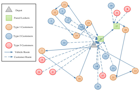
Figure 3.
Visual illustration of the example solution given in Figure 2.
The objective value is calculated based on the second row representing the real visited nodes of the vehicle. If there is time window and/or capacity violation, the vehicle needs to return to the depot without visiting the node. The following vehicle departs from the depot to service the sequential node until the final node is the depot. If the number of vehicles used exceeds the total number of vehicles, the solution is not feasible. Therefore, to avoid generating an infeasible solution, we implement a penalty policy.
4.2. Initial Solution
The process of constructing an initial solution consists of two steps. First, all customers are assigned to a specific delivery mode based on the type of customer. For example, a type 1 customer is assigned to home delivery and type 2 customer to the selected parcel locker station. Type 3 customer belongs to the home or locker delivery also attached to the parcel locker chosen station.
Step two utilizes the nearest neighborhood algorithm to select the closest node according to the currently visited node among the unassigned nodes. This algorithm terminates if all customer nodes have been assigned.
4.3. Neighborhood Moves
In the VRPSPDPL, the neighborhood solutions were obtained by applying three traditional types of movement methods: (1) swap, (2) insertion, (3) 2-opt *, and (4) change parcel locker. The swap move combines the relocation and exchange move, shifting a customer from one route to a different position in the same or different route [23]. The procedure randomly chooses and swaps two nodes to change the positions. The insertion move selects two nodes that are not adjacent, removes one node from its current location, and then inserts it after another node. The 2-opt * removes two arcs from two different routes to separate each route into two parts and swaps the ends of the two routes [23]. It generates two depots to divide the route into two parts: the original depot and the virtual depot. The destroyed points are at the end of two parts and then they swap routes. The change parcel locker is performed by randomly choosing a type 2 or type 3 customer and randomly choosing which locations can be used for the vehicle.
4.4. Simulated Annealing (SA) Procedure
The SA is performed after an initial solution is constructed. In the beginning, we set several parameters: is the current temperature, is the initial temperature, and is the final temperature that stops the SA procedure if the current temperature is below or equal to the final temperature; is the number of iterations, is the maximum number of iterations, is non-improving times, and is the maximum non-improving times that the best solution has not improved for consecutive temperature reductions; is the coefficient controlling the cooling schedule; is the Boltzmann constant.
Two types of solutions are kept during the iterations of SA, which represents the current solution and represents the best-found solution. Initially, is obtained from the initial solution and is set to . In each iteration, a new solution is generated from one of the four neighborhoods, as the above-mentioned moves. The way of selecting these moves is based on the randomly generated value, , ranging from 0 to 1. If is less than 1/4, swap is selected. If is between 1/4 and 1/2, insertion is selected. If is between 1/2 and 3/4, 2-Opt* is chosen. Otherwise, change in parcel locker is chosen.
After is generated, the objective value of is calculated, let represent the objective value of a solution to determine whether the is accepted as the new , a comparison between and is necessary; consequently, is defined as . The objective of VRPSPDPL is to minimize the travelled distance; therefore, is accepted when it has a lower objective value, which means . Moreover, if , is accepted as new . If results in a higher objective value, it is not directly rejected. A random value, , ranging from 0 to 1, is generated. If , is accepted as a new . Otherwise, is rejected. After an inner iteration cycle is completed, is reduced by multiplying with a constant . In the version of SA with backtrack (SAwb), the is set to equal to , while SA without backtracking (SA) does not have this step.
Before another inner iteration cycle starts, it is necessary to check whether the termination condition has been met. Figure 4 presents the procedure of the proposed SA.

Figure 4.
Simulated annealing procedure.
5. Experimental Results and Discussion
The proposed SA algorithm was implemented in C++ and run on a computer with an Intel® Core™ i7-4770 processor at 3.4 GHz and 8 GB of RAM under Windows 10 operation system. We tested the proposed SA algorithm on SDPPTW benchmark instances and the new instances for VRPSPDPL. The mathematical programming model for VRPSPDPL was solved using the Gurobi solver.
5.1. Test Instances
The instances for VRPSPDPL are modified from SDPPTW benchmark instances of Wang and Chen [13]. The SDPPTW instances were adopted from Solomon’s VRPTW instances [27]. Solomon’s test problem comprises six different types of problems: C1, C2, R1, R2, RC1, and RC2. The different properties at the coordinates, demands, and time windows are: C is with clustered customers, R is with locations of customers generated uniformly randomly, RC is a combination of randomly placed and clustered customers. The type 1 customer has limited time windows and small vehicle capacities, while the type 2 customer has large time windows and significant vehicle capacities. These instances are generated to three 10-customer problems, three 25-customer problems, three 50-customer problems, and fifty-six 100-customer problems. Wang and Chen [13] analyzed the trade-off parameter λ to adjust the different decision criteria. The parameter is a trade-off between two objective functions: the primary objective is to minimize the number of vehicles and the secondary aim is to minimize the total distance or travel time. However, the objective function of this research only focused on the total traveling cost. The benchmark instances for VRPSPDPL can be downloaded from http://web.ntust.edu.tw/~vincent/vrpspdpl/ (accessed on 10 March 2022).
5.2. Computational Results
This section illustrates the effectiveness of the proposed algorithm. There is no earlier published benchmark dataset for VRPSPDPL. However, VRPSPDPL is similar to the simultaneous delivery and pickup problem with the time window, except for the parcel lockers and customers. As a result, the performance of the proposed SA is evaluated by solving the SDPPTW dataset and then comparing the results with the solutions reported by Wang and Chen [13]. Next, the proposed SA was used to solve the VRPSPDPL datasets. The results of VRPSPDPL were compared with those obtained by Gurobi.
5.2.1. First Dataset—SDPPTW Dataset
The proposed SA was tested on SDPPTW instances. Table 1 and Table A1 summarize results for SDPPTW datasets: small, medium, and large instances. We compared the proposed SA, SA with backtrack, and Gurobi solutions with the GA algorithm by Wang and Chen [13]. In Table 1 and Table A1, NV represents the number of vehicles, TD represents the solution obtained, and CPU represents the computational time. We also calculated the Gap (percentage differences) between SA, SA with backtrack, Gurobi, and GA using the following formula:
Gap a: Gap a(%) = ((SA best objective value − GA)/GA) × 100%
Gap b: Gap b(%) = ((SAwb best objective value − GA)/GA) × 100%
Gap c: Gap c(%) = ((Gurobi objective value − GA)/GA) × 100%

Table 1.
Computational results for small and medium SDPPTW instances.
According to Table 1, the numbers of customers were 10, 25, and 50, respectively. The proposed SA and SAwb outperformed that of Wang and Chen [13], with the largest gap of −21.76% from solving the RCdp1007 dataset. However, Wang and Chen [13] outperform SA and SAwb with the largest gap of 1.10% and 1.05% from solving the RCdp5004 dataset. For 10 and 25 customers, the proposed SA and SAwb algorithm obtained a similar solution with Gurobi and outperformed the GA algorithm proposed by Wang and Chen [13] in terms of solution quality. For the results of 50 customers, there is one solution each better than GA, worse than GA. However, the solutions and CPU time of the proposed SA compared with Gurobi were found to be better. The solution of RCdp2504 and Rdcp2507 is not optimal for Gurobi, although it takes 5 h of solving time. The average CPU time of the proposed SA and SAwb is 8.91 and 10.29 s and the average gap is −2.55% and −2.56%, respectively. The negative value of the gap indicates that the proposed SA and SAwb are competitive with the method proposed by Wang and Chen [13].
According to Table A1, for each instance, there were 100 customers and each dataset contains two types of time windows, narrow and large time windows. The proposed SA and SAwb outperform GA proposed by Wang and Chen [13], with the largest gap of −18.88% and −19.70% by solving the RCdp201 dataset. However, GA outperformed SA with the largest gap of 3.62% from solving the Cdp204 dataset and outperformed SAwb with the largest gap of 1.36% by solving the Rdp109 dataset. Therefore, the proposed SA and Sawb algorithm provides a competitive result for narrow time windows. The proposed SA outperformed large time windows in terms of solution quality. The CPU time was, on average, 245.61 and 235.20 s, and the average gaps were −1.76% and −2.85% (better than BKS), for SA and SAwb, respectively.
On the other hand, based on Table A1, the Gurobi solver only provides a solution for 8 of 56 instances. Moreover, Gurobi solutions for Rdp208, Cdp101, Cdp207, RCdp203, RCdp204, and RCdp208 are not optimal solutions in 5 h of solving time. It can be found that the average gap of SAwb is better than that of the original SA. That is, with the backtracking mechanism, the quality of the original SA is improved.
5.2.2. The Second Dataset—VRPSPDPL
To the best of our best knowledge, VRPSPDPL has not been studied. Therefore, the results from the proposed SA and SAwb are compared with those obtained from Gurobi. The commercial solver Gurobi was terminated after 5 h if it could not find an optimal solution. Table 2 and Table A2 report the computational results for the number of vehicles, the best objective value, CPU time, and the gap between the proposed SA, SAwb, Gurobi, and best-known solution (BKS). BKS is the best solution among SA, SAwb, and Gurobi. The Gap (percentage difference) is computed between SA and Gurobi using the formula:
Gap d: Gap d(%) = ((Gurobi objective value − BKS)/BKS) × 100%
Gap e: Gap e(%) = ((SA best objective value − BKS)/BKS) × 100%
Gap f: Gap f(%) = ((SAwb best objective value − BKS)/BKS) × 100%
Table 2.
Computational results for small- and medium-sized VRPSPDPL instances.
Table 2 summarizes the results in VRPSPDPL for small and medium-size instances; the number of customers is 10, 25, and 50, respectively. It can be seen that both the proposed SA and SAwb obtain seven solutions that have the same value as the Gurobi solver, e.g., nRCdp1001, nRCdp1004, nRCdp1007, nRCdp2501, nRCdp2504, nRCdp2507, and nRCdp5001. Two solutions of the proposed SA and SAwb are better than those of Gurobi, namely, nRCdp5004 and nRCdp5007. However, the proposed SA works faster than Gurobi for medium-size problems. Among the nine instances, Gurobi cannot obtain the optimal solutions to five instances within 5 h. The average CPU time for SA and SAwb is 10.57 and 9.19 s, respectively. The average percentage gap is 0.21% and 0.00% for SA and SAwb, respectively. The solution quality of SAwb is a little better than that of SA when solving the small-scaled problem.
Table A2 presents the results for large sizes in VRPSPDPL. The number of customers is 100 for each instance. We can see that the Gurobi is only able to obtain a solution for 29 instances within 5 h. However, the solutions obtained were worse than both SA and SAwb. SA outperformed SAwb with the largest gap of 2.29% for solving the nCdp208 instance. However, SAwb outperformed SA with the largest gap of 8.60% for solving the nCdp104 instance. The average gap was 1.20% and 0.27% for SA and SAwb, respectively, indicating that the average gap of SAwb is better than the original SA. Moreover, the computational time required for SA was 281.69 and that for SAwb was 267.27 s, which indicates that SAwb is faster than SA on average to solve large instances.
We observed that by implementing SA with the backtracking mechanism, the solution quality for the original SA improved. Furthermore, for large instances, the proposed SAwb and SA had better solution quality than Gurobi.
5.3. Sensitivity Analysis for SA Parameters
The purpose of sensitivity analysis was to investigate the relationship between SA parameters and the quality of results obtained. We examined the effect of the initial temperature (), final temperature (), number of maximum iterations (), the coefficient controlling the cooling schedule (), the maximum non-improving times (), and Boltzmann constant (), on the average CPU time and average %Gap for SA. The initial parameter values that we applied in SA are as follows ; ; ; ; ; .
Figure A1 presents the effect of SA parameters on average CPU time and average %Gap of the result. The higher increased the probability of obtaining a better solution, but it also increased the computational time. This condition was also applied when the value of was reduced. When decreased from 0.1 to 0.01, the solution and computational time changed apparently.
The increasing provides a better solution until a particulate number of . Thus, the needs to be determined precisely to produce a good solution within considerable time.
The value of increased in increments of 0.01, starting from 0.97 to 0.99. This shows that increasing can lead to a better solution but at a longer computational time. However, the result was different after equals 0.98. Therefore, in our algorithm, the best used was 0.98.
Figure A1 also shows that the increase in value of increases the probability of obtaining a better solution, but it will consume more CPU time. However, the trend of the solution indicates that does not significantly affect the solution quality.
We also wanted to assess the effect of Boltzmann constant on the CPU time and solution quality. Therefore, several experiments were carried out with the values of 1/5, 1/3, and 1. Figure A1 shows that decreasing the Boltzmann’s constant can obtain a better solution but more CPU time.
5.4. Discussion
In this research, we proposed a mathematical programming model for VRPSPDPL. Besides the VRPSPDPL, the mathematical model can also solve another VRP variant, i.e., SDPPTW. However, to implement VRPSPDPL, we need to adjust constraints, parameters, decision variables, and assumptions because SDPPTW only considers one type of customer, i.e., the type 1 customer. Thus, the VRPSPDPL model could solve the problem for SDPPTW.
Although other types of models exist, such as stochastic and multi-objective programming models, which may be more appropriate for VRPSPDPL configuration, this research implements a mixed-integer programming model to formulate the VRPSPDPL. Other models face an issue in computational complexity [42]. Our model has advantages in providing a relatively simple and compact approximation of complex VRPSPDPL. However, we also note some important limitations in our proposed model. Compared with simulation, our mathematical model has a lower level of validity. It also has difficulties representing the dynamic and stochastic aspects of real-world cases, i.e., the capacity of each parcel locker. Therefore, to overcome these drawbacks, management and decision-makers must acquire accurate data, such as information on the availability of parcel lockers.
Based on the experiments, the mathematical model was solved using a commercial solver and metaheuristic. As shown in Table A1 and Table A2, it is difficult to provide optimal or feasible solutions using the commercial solver, e.g., Gurobi, as the size of the instances is larger. Although we already limited the computational time to 5 h, due to the complexity of the problem, the exact solver was only able to provide 8 of 56 SDPPTW instances and 29 of 56 VRPSPDPL instances. This condition becomes crucial if we want to implement the method into a real application with large datasets. Therefore, we were able to solve this drawback by developing a metaheuristic approach. However, using the result obtained from the exact solver, we could evaluate the performance of the proposed heuristic, i.e., simulated annealing.
Although the developed SA provides a competitive solution and reasonable computation time (Table 1 and Table 2, Table A1 and Table A2), we agree that each algorithm has its limitations. Our proposed SA may perform well in solving SDPPTW and VRPSPDPL, but the performance cannot be generalized to all problems before further experiments are conducted.
This paper proposes a metaheuristic approach to provide a good result and minimize computational time. However, the disadvantages of metaheuristics are the weak local search and the role of randomness. In this study, to deal with this drawback, we choose SA because it is appropriate with the structural characteristic of the VRPSPDPL. Moreover, to handle the critical factor in implementing the SA algorithm, we set the parameters to improve each iteration’s local search movement. Our SA can provide results within a reasonable time and the quality of the result is not too far from the optimal solution. The CPU run time indicates that the algorithm efficiently solves the VRPSPDPL. One weakness of our SA is that the difficulties of setting the SA parameters will provide a high-quality solution; therefore, the algorithm might not perform well if we modified the problem or added more extensions to the model.
The critical factors in implementing the SA algorithm to provide a good solution for VRPSPDPL are utilizing a set of neighborhood moves, the acceptance criterion, and parameter-tuning [17]. By utilizing various neighborhood moves, the SA could explore a wide range of solution spaces to find a promising solution. The acceptance criterion utilized in the SA enables the algorithm to avert the local optimal solutions. Moreover, by implementing a backtracking mechanism, SA could exploit the process to find a better solution.
In this research, statistical tests were also conducted to examine the significant result of the proposed algorithm. We implement the Wilcoxon signed-rank test to measure and analyze the results. We used the confidence level of alpha equal to 0.05 or 95% to test the hypothesis. In the case of p-value less than alpha, we conclude a significant difference from the methods. Table 3 and Table 4 show the result of the Wilcoxon signed-rank test for the SDPPTW and VRPSPDPL datasets, respectively.
Table 3.
Results of Wilcoxon signed-rank tests on solution value and running time for the SDPPTW dataset.
Table 4.
Results of Wilcoxon signed-rank tests on solution value and running time for the VRPSPDPL dataset.
As mentioned in Table 3, for almost all the results, the p-value is more than alpha. This means the difference between the results provided by the proposed SA is non-significant, compared to those by GA and Gurobi when solving SDPPTW. It also indicates that, statistically, our algorithm is capable of providing a competitive solution, compared with the original approach, i.e., GA. On the other hand, the developed VRPSPDPL mathematical model can also answer the problem of the SDPPTW because using the data provided by SDPPTW and the results are non-significantly different from the GA results.
As mentioned in Table 4, for the small and medium datasets, in terms of solution value, the p-value is larger than alpha, indicating weak evidence against the null hypothesis, which also means there is no significant difference in the result provided by our proposed algorithms. For the larger VRPSPDPL datasets, the p-value was 0.018, that is, less than alpha for the test on running time (SA vs. BKS), also indicating that there is a significant difference in running time. However, for SAwb vs. BKS, the p-value was 0.543, which means there is no significant difference between SAwb and BKS in terms of running time.
The results for Wilcoxon signed-rank for SAwb and SA are presented in Table 5. According to Table 5, SAwb significantly outperforms the SA in terms of solution value for large datasets, e.g., SDPPTW and VRPSPDPL datasets. Moreover, for VRPSPDPL, SAwb is significantly faster in solving large datasets.
Table 5.
Results of the Wilcoxon signed-rank tests on solution value and running time for SA and SAwb.
6. Conclusions
The research proposed VRPSPDPL and developed a mathematical model to solve the problem in last-mile delivery. The objective was to use SA to solve the problem and minimize the total traveling cost. VRPSPDPL divides the customers into three types: home delivery and pickup, parcel locker delivery and pickup, and home delivery or parcel locker delivery. However, home delivery and pickup can only be done in a specific period and there are no time windows for parcel lockers.
The performance of the proposed SA and SAwb was analyzed in solving both SDPPTW and VRPSPDPL benchmark instances. For SDPPTW, small- and medium-size instances, SA and SAwb, could obtain the largest gap of −21.76%, compared with the best-known solution. For SDPPTW large-size instances, SA and SAwb outperformed GA with the largest gaps of −18.88 and −19.70%. The results indicate that our proposed algorithm provides results comparable to those by available SDPPTW instances.
For the VRPSPDPL, the numerical study shows that the percentage gap between the best-known solution and the best objective value obtained by both the proposed SA and SAwb can obtain a slightly better solution than Gurobi in small- and medium-size instances. For large-size instances, both the proposed SA and SAwb can provide a much better solution than Gurobi. Furthermore, the average gap of SAwb was observed to be better than that of SA, that is, with the backtracking mechanism, the quality of the original SA is improved.
For future studies, VRPSPDPL could be combined with other situations or variants to make the model more realistic, such as heterogeneous vehicles, electric vehicles, or considering the locations or number of parcel lockers. Besides, future research can develop exact methods that might help confirm the optimal solution for large instances of the proposed problem.
Author Contributions
Conceptualization, V.F.Y. and Y.-H.Y.; methodology, V.F.Y., H.S., Y.-H.Y. and S.-W.L.; software, H.S., Y.-H.Y. and S.-W.L.; validation, V.F.Y., H.S. and Y.-T.H.; formal analysis, H.S.; investigation, Y.-H.Y.; resources, V.F.Y., S.-W.L. and Y.-T.H.; data curation, Y.-H.Y. and H.S.; writing—original draft preparation, V.F.Y., Y.-H.Y. and H.S.; writing—review and editing, V.F.Y., H.S., S.-W.L. and Y.-T.H.; visualization, Y.-H.Y. and H.S.; supervision, V.F.Y. and S.-W.L.; project administration, V.F.Y.; funding acquisition, V.F.Y. and S.-W.L. All authors have read and agreed to the published version of the manuscript.
Funding
This research was partially supported by the Ministry of Science and Technology of the Republic of China (Taiwan) under grant MOST 106-2410-H-011-002-MY3 and the Center for Cyber-Physical System Innovation from The Featured Areas Research Center Program within the framework of the Higher Education Sprout Project by the Ministry of Education (MOE) in Taiwan. The work of S.-W. Lin was supported in part by the Ministry of Science and Technology, Taiwan, under Grant MOST 109-2410-H-182-009MY3, and in part by the Linkou Chang Gung Memorial Hospital under Grant BMRPA19.
Institutional Review Board Statement
Not applicable.
Informed Consent Statement
Not applicable.
Data Availability Statement
Not applicable.
Conflicts of Interest
The authors declare no conflict of interest.
Appendix A
Table A1.
Computational results for large SDPPTW instances.
Table A1.
Computational results for large SDPPTW instances.
| Problem | GA | SA | SA with Backtrack | Gurobi | ||||||||||
|---|---|---|---|---|---|---|---|---|---|---|---|---|---|---|
| NV | TD | NV | TD | CPU | Gap a | NV | TD | CPU | Gap b | NV | TD | CPU | Gap c | |
| Rdp101 | 19 | 1653.53 | 20 | 1648.22 | 275.45 | −0.32% | 20 | 1646.15 | 236.15 | −0.45% | 20 | 1642.87 | 4657.68 | −0.64% |
| Rdp102 | 17 | 1488.04 | 19 | 1492.72 | 277.40 | 0.31% | 19 | 1484.59 | 224.16 | −0.23% | N/A | N/A | 18,000 | N/A |
| Rdp103 | 14 | 1216.16 | 15 | 1239.29 | 278.34 | 1.90% | 15 | 1222.04 | 225.57 | 0.48% | N/A | N/A | 18,000 | N/A |
| Rdp104 | 10 | 1015.41 | 12 | 1004.76 | 279.89 | −1.05% | 12 | 1003.83 | 229.65 | −1.14% | N/A | N/A | 18,000 | N/A |
| Rdp105 | 15 | 1375.31 | 17 | 1400.14 | 274.73 | 1.81% | 16 | 1381.02 | 224.23 | 0.41% | N/A | N/A | 18,000 | N/A |
| Rdp106 | 13 | 1255.48 | 14 | 1261.73 | 279.79 | 0.50% | 14 | 1255.56 | 225.96 | 0.01% | N/A | N/A | 18,000 | N/A |
| Rdp107 | 11 | 1087.95 | 12 | 1102.92 | 236.58 | 1.38% | 11 | 1087.78 | 228.58 | −0.02% | N/A | N/A | 18,000 | N/A |
| Rdp108 | 10 | 967.49 | 11 | 969.41 | 234.18 | 0.20% | 11 | 962.43 | 228.98 | −0.52% | N/A | N/A | 18,000 | N/A |
| Rdp109 | 12 | 1160.00 | 13 | 1173.39 | 229.62 | 1.15% | 13 | 1175.79 | 224.36 | 1.36% | N/A | N/A | 18,000 | N/A |
| Rdp110 | 12 | 1116.99 | 13 | 1115.43 | 231.48 | −0.14% | 12 | 1103.45 | 224.06 | −1.21% | N/A | N/A | 18,000 | N/A |
| Rdp111 | 11 | 1065.27 | 12 | 1075.06 | 230.47 | 0.92% | 12 | 1067.81 | 224.66 | 0.24% | N/A | N/A | 18,000 | N/A |
| Rdp112 | 10 | 974.03 | 11 | 979.95 | 227.52 | 0.61% | 11 | 975.14 | 225.57 | 0.11% | N/A | N/A | 18,000 | N/A |
| Rdp201 | 4 | 1280.44 | 10 | 1176.46 | 230.72 | −8.12% | 8 | 1153.04 | 226.28 | −9.95% | N/A | N/A | 18,000 | N/A |
| Rdp202 | 4 | 1100.92 | 8 | 1060.30 | 234.32 | −3.69% | 8 | 1047.73 | 232.36 | −4.83% | N/A | N/A | 18,000 | N/A |
| Rdp203 | 3 | 950.79 | 6 | 898.40 | 237.45 | −5.51% | 6 | 881.77 | 252.30 | −7.26% | N/A | N/A | 18,000 | N/A |
| Rdp204 | 3 | 775.23 | 4 | 749.05 | 265.45 | −3.38% | 5 | 739.18 | 290.96 | −4.65% | N/A | N/A | 18,000 | N/A |
| Rdp205 | 3 | 1064.43 | 6 | 983.34 | 196.79 | −7.62% | 6 | 969.78 | 218.06 | −8.89% | N/A | N/A | 18,000 | N/A |
| Rdp206 | 3 | 961.32 | 6 | 908.56 | 188.23 | −5.49% | 6 | 906.69 | 234.60 | −5.68% | N/A | N/A | 18,000 | N/A |
| Rdp207 | 3 | 835.01 | 5 | 814.63 | 198.28 | −2.44% | 4 | 809.13 | 200.28 | −3.10% | N/A | N/A | 18,000 | N/A |
| Rdp208 | 3 | 718.51 | 4 | 731.39 | 194.61 | 1.79% | 4 | 708.88 | 220.45 | −1.34% | 16 | 2040.19 | 18,000 | 183.9% |
| Rdp209 | 3 | 930.26 | 6 | 890.15 | 166.72 | −4.31% | 6 | 874.53 | 172.13 | −5.99% | N/A | N/A | 18,000 | N/A |
| Rdp210 | 3 | 983.75 | 6 | 926.09 | 165.45 | −5.86% | 6 | 915.63 | 173.56 | −6.92% | N/A | N/A | 18,000 | N/A |
| Rdp211 | 3 | 839.61 | 5 | 775.07 | 171.97 | −7.69% | 5 | 761.28 | 179.12 | −9.33% | N/A | N/A | 18,000 | N/A |
| Cdp101 | 11 | 1001.97 | 12 | 963.96 | 284.24 | −3.79% | 12 | 965.46 | 240.13 | −3.64% | 12 | 982.02 | 18,000 | −1.99% |
| Cdp102 | 10 | 961.38 | 12 | 955.75 | 284.93 | −0.59% | 11 | 944.94 | 239.32 | −1.71% | N/A | N/A | 18,000 | N/A |
| Cdp103 | 10 | 897.65 | 11 | 888.56 | 286.97 | −1.01% | 11 | 887.47 | 227.90 | −1.13% | N/A | N/A | 18,000 | N/A |
| Cdp104 | 10 | 878.93 | 11 | 870.98 | 286.92 | −0.90% | 11 | 870.98 | 226.10 | −0.90% | N/A | N/A | 18,000 | N/A |
| Cdp105 | 11 | 983.10 | 12 | 991.63 | 283.26 | 0.87% | 12 | 991.57 | 226.32 | 0.86% | N/A | N/A | 18,000 | N/A |
| Cdp106 | 11 | 878.29 | 11 | 878.47 | 285.64 | 0.02% | 11 | 878.29 | 229.88 | 0.00% | N/A | N/A | 18,000 | N/A |
| Cdp107 | 11 | 913.81 | 12 | 908.99 | 233.18 | −0.53% | 12 | 908.99 | 232.11 | −0.53% | N/A | N/A | 18,000 | N/A |
| Cdp108 | 10 | 951.24 | 11 | 920.30 | 235.06 | −3.25% | 11 | 920.30 | 227.49 | −3.25% | N/A | N/A | 18,000 | N/A |
| Cdp109 | 10 | 940.49 | 11 | 926.55 | 231.02 | −1.48% | 11 | 928.06 | 228.68 | −1.32% | N/A | N/A | 18,000 | N/A |
| Cdp201 | 3 | 591.56 | 3 | 591.56 | 260.04 | 0.00% | 3 | 591.56 | 278.92 | 0.00% | 3 | 591.56 | 1075.78 | 0.00% |
| Cdp202 | 3 | 591.56 | 3 | 591.56 | 265.44 | 0.00% | 3 | 591.56 | 282.14 | 0.00% | N/A | N/A | 18,000 | N/A |
| Cdp203 | 3 | 591.17 | 4 | 607.24 | 265.12 | 2.72% | 3 | 591.17 | 281.61 | 0.00% | N/A | N/A | 18,000 | N/A |
| Cdp204 | 3 | 590.60 | 3 | 611.98 | 264.34 | 3.62% | 3 | 590.60 | 285.77 | 0.00% | N/A | N/A | 18,000 | N/A |
| Cdp205 | 3 | 588.88 | 3 | 588.88 | 259.93 | 0.00% | 3 | 588.88 | 277.67 | 0.00% | N/A | N/A | 18,000 | N/A |
| Cdp206 | 3 | 588.49 | 3 | 588.49 | 268.27 | 0.00% | 3 | 588.49 | 284.84 | 0.00% | N/A | N/A | 18,000 | N/A |
| Cdp207 | 3 | 588.29 | 3 | 595.10 | 225.99 | 1.16% | 3 | 588.29 | 255.42 | 0.00% | 17 | 1778.56 | 18,000 | 202.3% |
| Cdp208 | 3 | 588.32 | 3 | 593.52 | 213.99 | 0.88% | 3 | 588.32 | 254.51 | 0.00% | N/A | N/A | 18,000 | N/A |
| RCdp101 | 15 | 1652.90 | 18 | 1672.92 | 275.42 | 1.21% | 17 | 1654.08 | 238.62 | 0.07% | N/A | N/A | 18,000 | N/A |
| RCdp102 | 14 | 1497.05 | 16 | 1517.52 | 275.53 | 1.37% | 15 | 1491.31 | 225.52 | −0.38% | N/A | N/A | 18,000 | N/A |
| RCdp103 | 12 | 1338.76 | 13 | 1359.95 | 281.95 | 1.58% | 12 | 1336.33 | 227.24 | −0.18% | N/A | N/A | 18,000 | N/A |
| RCdp104 | 11 | 1188.49 | 11 | 1198.54 | 279.56 | 0.85% | 11 | 1177.98 | 228.05 | −0.88% | N/A | N/A | 18,000 | N/A |
| RCdp105 | 14 | 1581.26 | 17 | 1577.88 | 277.60 | −0.21% | 16 | 1566.18 | 229.32 | −0.95% | N/A | N/A | 18,000 | N/A |
| RCdp106 | 13 | 1422.87 | 14 | 1446.13 | 274.66 | 1.63% | 14 | 1400.42 | 227.39 | −1.58% | N/A | N/A | 18,000 | N/A |
| RCdp107 | 12 | 1282.10 | 13 | 1307.35 | 229.15 | 1.97% | 12 | 1264.31 | 226.45 | −1.39% | N/A | N/A | 18,000 | N/A |
| RCdp108 | 11 | 1175.04 | 12 | 1189.73 | 229.14 | 1.25% | 12 | 1161.61 | 229.27 | −1.14% | N/A | N/A | 18,000 | N/A |
| RCdp201 | 4 | 1587.92 | 10 | 1288.07 | 223.53 | −18.88% | 10 | 1275.10 | 230.47 | −19.70% | N/A | N/A | 18,000 | N/A |
| RCdp202 | 4 | 1211.12 | 8 | 1107.72 | 232.39 | −8.54% | 8 | 1103.72 | 233.20 | −8.87% | N/A | N/A | 18,000 | N/A |
| RCdp203 | 4 | 964.65 | 6 | 971.68 | 239.07 | 0.73% | 6 | 948.74 | 246.86 | −1.65% | 21 | 2439.31 | 18,000 | 152.9% |
| RCdp204 | 3 | 822.02 | 5 | 813.48 | 256.11 | −1.04% | 4 | 805.61 | 274.41 | −2.00% | 17 | 2117.45 | 18,000 | 157.6% |
| RCdp205 | 4 | 1410.18 | 10 | 1191.92 | 239.55 | −15.48% | 9 | 1173.73 | 224.02 | −16.77% | N/A | N/A | 18,000 | N/A |
| RCdp206 | 3 | 1176.85 | 7 | 1089.50 | 230.54 | −7.42% | 7 | 1062.49 | 231.47 | −9.72% | N/A | N/A | 18,000 | N/A |
| RCdp207 | 4 | 1036.59 | 7 | 999.16 | 231.87 | −3.61% | 6 | 975.47 | 239.84 | −5.90% | N/A | N/A | 18,000 | N/A |
| RCdp208 | 3 | 878.57 | 6 | 819.85 | 238.51 | −6.68% | 6 | 808.96 | 258.33 | −7.92% | 16 | 2479.13 | 18,000 | 182.2% |
| Average | 9.57 | 1017.88 | 245.61 | −1.76% | 9.30 | 1006.32 | 235.20 | −2.85% | 17,459.53 | |||||
Bold values denote the largest gap.
Table A2.
Computational results for large-size VRPSPDPL instances.
Table A2.
Computational results for large-size VRPSPDPL instances.
| Problem | BKS | CPU | Gurobi | SA | SA with Backtrack | ||||||||
|---|---|---|---|---|---|---|---|---|---|---|---|---|---|
| NV | TD | CPU | NV | TD | CPU | Gap | NV | TD | CPU | Gap | |||
| nRdp101 | 1036.66 | 256.20 | N/A | N/A | 18,000 | 13 | 1037.97 | 246.69 | 0.13% | 13 | 1036.66 | 256.20 | 0.00% |
| nRdp102 | 905.44 | 247.31 | N/A | N/A | 18,000 | 11 | 927.53 | 245.66 | 2.44% | 10 | 905.44 | 247.31 | 0.00% |
| nRdp103 | 726.49 | 247.59 | N/A | N/A | 18,000 | 9 | 734.47 | 248.69 | 1.10% | 9 | 726.49 | 247.59 | 0.00% |
| nRdp104 | 688.23 | 248.32 | N/A | N/A | 18,000 | 9 | 699.44 | 251.24 | 1.63% | 9 | 688.23 | 248.32 | 0.00% |
| nRdp105 | 838.41 | 247.95 | N/A | N/A | 18,000 | 10 | 857.70 | 249.81 | 2.30% | 10 | 838.41 | 247.95 | 0.00% |
| nRdp106 | 768.71 | 246.98 | 16 | 1351.99 | 18,000 | 10 | 768.71 | 252.08 | 0.00% | 10 | 768.87 | 246.98 | 0.02% |
| nRdp107 | 793.03 | 247.88 | N/A | N/A | 18,000 | 10 | 793.03 | 247.88 | 0.00% | 10 | 802.17 | 243.48 | 1.15% |
| nRdp108 | 690.78 | 245.64 | 14 | 1360.24 | 18,000 | 10 | 690.78 | 245.64 | 0.00% | 9 | 695.08 | 248.45 | 0.62% |
| nRdp109 | 805.26 | 245.81 | N/A | N/A | 18,000 | 11 | 816.58 | 253.60 | 1.41% | 10 | 805.26 | 245.81 | 0.00% |
| nRdp110 | 750.84 | 249.74 | N/A | N/A | 18,000 | 10 | 750.84 | 249.74 | 0.00% | 9 | 762.86 | 247.44 | 1.60% |
| nRdp111 | 757.36 | 244.40 | N/A | N/A | 18,000 | 9 | 769.84 | 256.43 | 1.65% | 9 | 757.36 | 244.40 | 0.00% |
| nRdp112 | 582.62 | 241.58 | N/A | N/A | 18,000 | 10 | 603.43 | 249.21 | 3.57% | 9 | 582.62 | 241.58 | 0.00% |
| nRdp201 | 661.74 | 298.35 | 6 | 689.37 | 18,000 | 6 | 661.74 | 298.35 | 0.00% | 6 | 662.01 | 294.60 | 0.04% |
| nRdp202 | 571.60 | 304.50 | 8 | 805.05 | 18,000 | 5 | 575.87 | 315.60 | 0.75% | 5 | 571.60 | 304.50 | 0.00% |
| nRdp203 | 523.52 | 322.82 | 9 | 817.04 | 18,000 | 3 | 523.52 | 322.82 | 0.00% | 3 | 523.52 | 327.74 | 0.00% |
| nRdp204 | 412.39 | 340.70 | 4 | 620.49 | 18,000 | 2 | 412.39 | 382.17 | 0.00% | 2 | 412.39 | 340.70 | 0.00% |
| nRdp205 | 553.45 | 267.40 | 8 | 951.21 | 18,000 | 4 | 553.45 | 312.92 | 0.00% | 4 | 553.45 | 267.40 | 0.00% |
| nRdp206 | 526.67 | 256.78 | 7 | 659.28 | 18,000 | 4 | 526.85 | 233.39 | 0.03% | 4 | 526.67 | 256.78 | 0.00% |
| nRdp207 | 510.68 | 239.76 | 6 | 741.78 | 18,000 | 3 | 525.04 | 390.05 | 2.81% | 3 | 510.68 | 239.76 | 0.00% |
| nRdp208 | 457.36 | 298.67 | 6 | 866.135 | 18,000 | 3 | 459.11 | 417.75 | 0.38% | 3 | 457.36 | 298.67 | 0.00% |
| nRdp209 | 564.10 | 238.75 | 7 | 989.10 | 18,000 | 4 | 570.14 | 362.37 | 1.07% | 4 | 564.10 | 238.75 | 0.00% |
| nRdp210 | 523.54 | 240.84 | 6 | 655.00 | 18,000 | 4 | 523.54 | 366.74 | 0.00% | 4 | 523.54 | 240.84 | 0.00% |
| nRdp211 | 443.32 | 276.04 | 4 | 734.09 | 18,000 | 3 | 443.32 | 409.94 | 0.00% | 3 | 443.32 | 276.04 | 0.00% |
| nCdp101 | 978.43 | 256.03 | N/A | N/A | 18,000 | 14 | 1056.71 | 240.81 | 8.00% | 13 | 978.43 | 256.03 | 0.00% |
| nCdp102 | 946.20 | 241.52 | N/A | N/A | 18,000 | 12 | 946.20 | 241.52 | 0.00% | 11 | 947.13 | 246.01 | 0.10% |
| nCdp103 | 825.63 | 244.63 | N/A | N/A | 18,000 | 11 | 869.74 | 245.65 | 5.34% | 11 | 825.63 | 244.43 | 0.00% |
| nCdp104 | 817.54 | 243.68 | N/A | N/A | 18,000 | 11 | 887.85 | 243.17 | 8.60% | 10 | 817.54 | 243.68 | 0.00% |
| nCdp105 | 978.68 | 242.23 | N/A | N/A | 18,000 | 11 | 988.51 | 241.56 | 1.00% | 11 | 978.68 | 242.23 | 0.00% |
| nCdp106 | 884.00 | 244.93 | N/A | N/A | 18,000 | 12 | 894.70 | 246.53 | 1.21% | 11 | 884.00 | 244.93 | 0.00% |
| nCdp107 | 945.54 | 243.82 | N/A | N/A | 18,000 | 12 | 945.54 | 243.82 | 0.00% | 11 | 950.86 | 244.83 | 0.56% |
| nCdp108 | 890.65 | 243.66 | N/A | N/A | 18,000 | 11 | 893.18 | 242.96 | 0.28% | 11 | 890.65 | 243.66 | 0.00% |
| nCdp109 | 779.69 | 239.45 | N/A | N/A | 18,000 | 11 | 845.98 | 242.21 | 8.50% | 11 | 779.69 | 239.45 | 0.00% |
| nCdp201 | 552.43 | 299.52 | N/A | N/A | 18,000 | 4 | 552.43 | 299.52 | 0.00% | 4 | 553.06 | 295.61 | 0.11% |
| nCdp202 | 463.54 | 325.96 | 5 | 649.149 | 18,000 | 3 | 463.54 | 325.96 | 0.00% | 3 | 470.95 | 321.69 | 1.60% |
| nCdp203 | 529.31 | 300.15 | 11 | 1338.35 | 18,000 | 4 | 543.82 | 305.28 | 2.74% | 4 | 529.31 | 300.15 | 0.00% |
| nCdp204 | 471.88 | 328.32 | 9 | 922.49 | 18,000 | 3 | 474.37 | 328.38 | 0.53% | 3 | 471.88 | 328.32 | 0.00% |
| nCdp205 | 575.83 | 299.99 | 8 | 918.10 | 18,000 | 4 | 578.15 | 307.06 | 0.40% | 4 | 575.83 | 299.99 | 0.00% |
| nCdp206 | 480.55 | 306.25 | 10 | 972.10 | 18,000 | 3 | 480.55 | 306.25 | 0.00% | 3 | 487.23 | 288.68 | 1.39% |
| nCdp207 | 547.57 | 287.36 | 7 | 792.38 | 18,000 | 4 | 556.96 | 294.44 | 1.71% | 4 | 547.57 | 287.36 | 0.00% |
| nCdp208 | 546.47 | 235.37 | 9 | 1099.83 | 18,000 | 4 | 546.47 | 235.37 | 0.00% | 4 | 558.97 | 230.60 | 2.29% |
| nRCdp101 | 1144.00 | 254.03 | N/A | N/A | 18,000 | 13 | 1161.79 | 242.20 | 1.56% | 12 | 1144.00 | 254.03 | 0.00% |
| nRCdp102 | 1130.27 | 244.11 | N/A | N/A | 18,000 | 11 | 1130.27 | 243.21 | 0.00% | 11 | 1130.31 | 244.11 | 0.00% |
| nRCdp103 | 1010.00 | 243.13 | N/A | N/A | 18,000 | 11 | 1018.62 | 242.34 | 0.85% | 11 | 1010.00 | 243.13 | 0.00% |
| nRCdp104 | 965.87 | 246.51 | N/A | N/A | 18,000 | 10 | 1012.17 | 241.29 | 4.79% | 10 | 965.87 | 246.51 | 0.00% |
| nRCdp105 | 1098.33 | 242.04 | N/A | N/A | 18,000 | 12 | 1098.33 | 242.04 | 0.00% | 12 | 1100.01 | 244.15 | 0.15% |
| nRCdp106 | 1046.62 | 244.88 | N/A | N/A | 18,000 | 11 | 1058.63 | 254.34 | 1.15% | 11 | 1046.62 | 244.88 | 0.00% |
| nRCdp107 | 1003.83 | 245.84 | 20 | 2184.07 | 18,000 | 11 | 1003.83 | 245.84 | 0.00% | 11 | 1010.14 | 243.41 | 0.63% |
| nRCdp108 | 1028.61 | 239.71 | N/A | N/A | 18,000 | 11 | 1028.61 | 239.71 | 0.00% | 10 | 1035.37 | 243.31 | 0.66% |
| nRCdp201 | 798.99 | 307.14 | 8 | 1060.53 | 18,000 | 6 | 798.99 | 307.14 | 0.00% | 5 | 809.70 | 302.30 | 1.34% |
| nRCdp202 | 722.47 | 291.48 | 7 | 951.63 | 18,000 | 6 | 729.17 | 288.95 | 0.93% | 6 | 722.47 | 291.48 | 0.00% |
| nRCdp203 | 610.50 | 300.56 | 5 | 789.801 | 18,000 | 4 | 610.88 | 296.27 | 0.06% | 4 | 610.50 | 300.56 | 0.00% |
| nRCdp204 | 522.77 | 341.21 | 9 | 1270.22 | 18,000 | 2 | 522.77 | 341.21 | 0.00% | 2 | 529.53 | 371.76 | 1.29% |
| nRCdp205 | 683.63 | 305.78 | 7 | 838.164 | 18,000 | 5 | 683.63 | 305.78 | 0.00% | 5 | 689.00 | 318.08 | 0.78% |
| nRCdp206 | 737.78 | 300.17 | 10 | 1136.98 | 18,000 | 4 | 737.78 | 300.17 | 0.00% | 5 | 738.92 | 308.32 | 0.16% |
| nRCdp207 | 685.44 | 287.00 | 7 | 1086.28 | 18,000 | 5 | 685.44 | 287.00 | 0.00% | 5 | 687.18 | 259.98 | 0.25% |
| nRCdp208 | 621.02 | 297.67 | 7 | 1143.21 | 18,000 | 3 | 621.02 | 297.67 | 0.00% | 4 | 624.48 | 242.22 | 0.56% |
| Average | 18,000 | 7.54 | 743.78 | 281.69 | 1.20% | 7.34 | 736.06 | 267.27 | 0.27% | ||||
Bold values denote the largest gap.
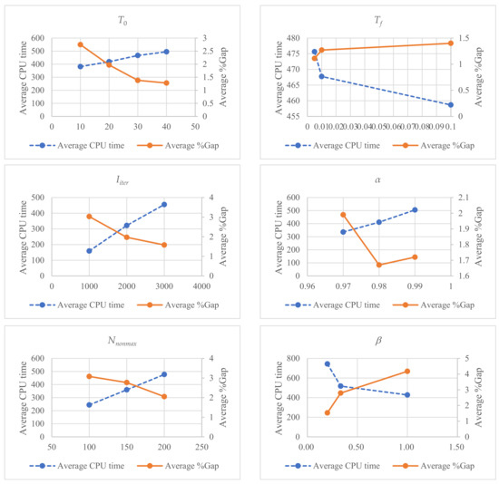
Figure A1.
Effect of SA parameters (, , , , , and ) on average CPU time and average %Gap.
References
- Agatz, N.A.; Fleischmann, M.; Van Nunen, J.A. E-fulfillment and multi-channel distribution—A review. Eur. J. Oper. Res. 2008, 187, 339–356. [Google Scholar] [CrossRef] [Green Version]
- Janjevic, M.; Winkenbach, M. Characterizing urban last-mile distribution strategies in mature and emerging e-commerce markets. Transp. Res. Part A Policy Pract. 2020, 133, 164–196. [Google Scholar] [CrossRef]
- Deutsch, Y.; Golany, B. A parcel locker network as a solution to the logistics last mile problem. Int. J. Prod. Res. 2018, 56, 251–261. [Google Scholar] [CrossRef]
- Zhou, L.; Wang, X.; Ni, L.; Lin, Y. Location-routing problem with simultaneous home delivery and customer’s pickup for city distribution of online shopping purchases. Sustainability 2016, 8, 828. [Google Scholar] [CrossRef] [Green Version]
- Vakulenko, Y.; Hellström, D.; Hjort, K. What’s in the parcel locker? Exploring customer value in e-commerce last mile delivery. J. Bus. Res. 2018, 88, 421–427. [Google Scholar] [CrossRef]
- Lee, H.; Chen, M.; Pham, H.T.; Choo, S. Development of a Decision Making System for Installing Unmanned Parcel Lockers: Focusing on Residential Complexes in Korea. KSCE J. Civ. Eng. 2019, 23, 2713–2722. [Google Scholar] [CrossRef]
- Zhou, L.; Baldacci, R.; Vigo, D.; Wang, X. A multi-depot two-echelon vehicle routing problem with delivery options arising in the last mile distribution. Eur. J. Oper. Res. 2018, 265, 765–778. [Google Scholar] [CrossRef]
- Rozman, T. Lockers. In The Changing Postal Environment; Springer: Berlin/Heidelberg, Germany, 2020; pp. 281–292. [Google Scholar]
- Hornstra, R.P.; Silva, A.; Roodbergen, K.J.; Coelho, L.C. The vehicle routing problem with simultaneous pickup and delivery and handling costs. Comput. Oper. Res. 2020, 115, 104858. [Google Scholar] [CrossRef]
- Bortfeldt, A.; Yi, J. The Split Delivery Vehicle Routing Problem with three-dimensional loading constraints. Eur. J. Oper. Res. 2020, 282, 545–558. [Google Scholar] [CrossRef]
- Enthoven, D.L.; Jargalsaikhan, B.; Roodbergen, K.J.; uit het Broek, M.A.; Schrotenboer, A.H. The two-echelon vehicle routing problem with covering options: City logistics with cargo bikes and parcel lockers. Comput. Oper. Res. 2020, 118, 104919. [Google Scholar] [CrossRef]
- Lachapelle, U.; Burke, M.; Brotherton, A.; Leung, A. Parcel locker systems in a car dominant city: Location, characterisation and potential impacts on city planning and consumer travel access. J. Transp. Geogr. 2018, 71, 1–14. [Google Scholar] [CrossRef]
- Wang, H.-F.; Chen, Y.-Y. A genetic algorithm for the simultaneous delivery and pickup problems with time window. Comput. Ind. Eng. 2012, 62, 84–95. [Google Scholar] [CrossRef]
- Liu, R.; Xie, X.; Augusto, V.; Rodriguez, C. Heuristic algorithms for a vehicle routing problem with simultaneous delivery and pickup and time windows in home health care. Eur. J. Oper. Res. 2013, 230, 475–486. [Google Scholar] [CrossRef] [Green Version]
- Wang, X.; Zhan, L.; Ruan, J.; Zhang, J. How to choose “last mile” delivery modes for e-fulfillment. Math. Probl. Eng. 2014, 2014, 417129. [Google Scholar] [CrossRef]
- Dokeroglu, T.; Sevinc, E.; Kucukyilmaz, T.; Cosar, A. A survey on new generation metaheuristic algorithms. Comput. Ind. Eng. 2019, 137, 106040. [Google Scholar] [CrossRef]
- Normasari, N.M.E.; Yu, V.F.; Bachtiyar, C. A simulated annealing heuristic for the capacitated green vehicle routing problem. Math. Probl. Eng. 2019, 2019, 2358258. [Google Scholar] [CrossRef]
- Chiang, W.-C.; Russell, R.A. Simulated annealing metaheuristics for the vehicle routing problem with time windows. Ann. Oper. Res. 1996, 63, 3–27. [Google Scholar] [CrossRef]
- Yu, V.F.; Redi, A.A.N.P.; Hidayat, Y.A.; Wibowo, O.J. A simulated annealing heuristic for the hybrid vehicle routing problem. Appl. Soft Comput. 2017, 53, 119–132. [Google Scholar] [CrossRef]
- Kuo, Y. Using simulated annealing to minimize fuel consumption for the time-dependent vehicle routing problem. Comput. Ind. Eng. 2010, 59, 157–165. [Google Scholar] [CrossRef]
- Karagul, K.; Sahin, Y.; Aydemir, E.; Oral, A. A simulated annealing algorithm based solution method for a green vehicle routing problem with fuel consumption. In Lean and Green Supply Chain Management; Springer: Berlin/Heidelberg, Germany, 2019; pp. 161–187. [Google Scholar]
- Yu, V.F.; Winarno; Maulidin, A.; Redi, A.; Lin, S.-W.; Yang, C.-L. Simulated Annealing with Restart Strategy for the Path Cover Problem with Time Windows. Mathematics 2021, 9, 1625. [Google Scholar] [CrossRef]
- Wang, C.; Mu, D.; Zhao, F.; Sutherland, J.W. A parallel simulated annealing method for the vehicle routing problem with simultaneous pickup–delivery and time windows. Comput. Ind. Eng. 2015, 83, 111–122. [Google Scholar] [CrossRef]
- Angelelli, E.; Mansini, R. The vehicle routing problem with time windows and simultaneous pick-up and delivery. In Quantitative Approaches to Distribution Logistics and Supply Chain Management; Springer: Berlin/Heidelberg, Germany, 2002; pp. 249–267. [Google Scholar]
- Mingyong, L.; Erbao, C. An improved differential evolution algorithm for vehicle routing problem with simultaneous pickups and deliveries and time windows. Eng. Appl. Artif. Intell. 2010, 23, 188–195. [Google Scholar] [CrossRef]
- Fan, J. The vehicle routing problem with simultaneous pickup and delivery based on customer satisfaction. Procedia Eng. 2011, 15, 5284–5289. [Google Scholar] [CrossRef] [Green Version]
- Solomon, M.M. Algorithms for the vehicle routing and scheduling problems with time window constraints. Oper. Res. 1987, 35, 254–265. [Google Scholar] [CrossRef] [Green Version]
- Liu, S.; Tang, K.; Yao, X. Memetic Search for Vehicle Routing with Simultaneous Pickup-Delivery and Time Windows. Swarm Evol. Comput. 2021, 66, 100927. [Google Scholar] [CrossRef]
- Sitek, P.; Wikarek, J. Capacitated vehicle routing problem with pick-up and alternative delivery (CVRPPAD): Model and implementation using hybrid approach. Ann. Oper. Res. 2019, 273, 257–277. [Google Scholar] [CrossRef] [Green Version]
- Redi, A.A.N.P.; Jewpanya, P.; Kurniawan, A.C.; Persada, S.F.; Nadlifatin, R.; Dewi, O.A.C. A Simulated Annealing Algorithm for Solving Two-Echelon Vehicle Routing Problem with Locker Facilities. Algorithms 2020, 13, 218. [Google Scholar] [CrossRef]
- Koç, Ç.; Laporte, G.; Tükenmez, İ. A review of vehicle routing with simultaneous pickup and delivery. Comput. Oper. Res. 2020, 122, 104987. [Google Scholar] [CrossRef]
- Rohmer, S.; Gendron, B. A Guide to Parcel Lockers in Last Mile Distribution Highlighting Challenges and Opportunities from an OR Perspective; CIRRELT: Montreal, QC, Canada, 2020. [Google Scholar]
- Subramanian, A.; Drummond, L.M.d.A.; Bentes, C.; Ochi, L.S.; Farias, R. A parallel heuristic for the vehicle routing problem with simultaneous pickup and delivery. Comput. Oper. Res. 2010, 37, 1899–1911. [Google Scholar] [CrossRef]
- Fisher, M.L. Optimal solution of vehicle routing problems using minimum k-trees. Oper. Res. 1994, 42, 626–642. [Google Scholar] [CrossRef]
- Yu, V.F.; Lin, S.-W.; Lee, W.; Ting, C.-J. A simulated annealing heuristic for the capacitated location routing problem. Comput. Ind. Eng. 2010, 58, 288–299. [Google Scholar] [CrossRef]
- Seçkiner, S.U.; Kurt, M. A simulated annealing approach to the solution of job rotation scheduling problems. Appl. Math. Comput. 2007, 188, 31–45. [Google Scholar] [CrossRef]
- Siddique, N.; Adeli, H. Simulated annealing, its variants and engineering applications. Int. J. Artif. Intell. Tools 2016, 25, 1630001. [Google Scholar] [CrossRef]
- Johnson, D.S.; Aragon, C.R.; McGeoch, L.A.; Schevon, C. Optimization by simulated annealing: An experimental evaluation; part II, graph coloring and number partitioning. Oper. Res. 1991, 39, 378–406. [Google Scholar] [CrossRef] [Green Version]
- Wang, C.-H.; Lu, J.-Z. A hybrid genetic algorithm that optimizes capacitated vehicle routing problems. Expert Syst. Appl. 2009, 36, 2921–2936. [Google Scholar] [CrossRef]
- Assad, A.; Deep, K. A hybrid harmony search and simulated annealing algorithm for continuous optimization. Inf. Sci. 2018, 450, 246–266. [Google Scholar] [CrossRef]
- Kao, Y.; Chen, M. Solving the CVRP problem using a hybrid PSO approach. In Computational Intelligence; Springer: Berlin/Heidelberg, Germany, 2013; pp. 59–67. [Google Scholar]
- Chandra, C.; Grabis, J. Mathematical Programming Approaches. In Supply Chain Configuration Concepts, Solutions, and Applications; Springer: Boston, MA, USA, 2007; pp. 183–206. [Google Scholar]
Publisher’s Note: MDPI stays neutral with regard to jurisdictional claims in published maps and institutional affiliations. |
© 2022 by the authors. Licensee MDPI, Basel, Switzerland. This article is an open access article distributed under the terms and conditions of the Creative Commons Attribution (CC BY) license (https://creativecommons.org/licenses/by/4.0/).