Abstract
The dimensionality of parameters and variables is a fundamental issue in physics but is mostly ignored from a mathematical point of view. Difficulties arising from dimensional inconsistency are overcome by scaling analysis and, often, both concepts, dimensionality and scaling, are confused. In the particular case of iterative methods for solving nonlinear equations, dimensionality and scaling affect their robustness: While some classical methods, such as Newton’s, are adimensional and scale independent, some other iterations such as Steffensen’s are not; their convergence depends on scaling, and their evaluation needs a dimensional congruence. In this paper, we introduce the concept of an adimensional form of a function in order to study the behavior of iterative methods, thus correcting, if possible, some pathological features. From this adimensional form, we will devise an adimensional and scale invariant method based on Steffensen’s, which we will call the ASIS method.
Keywords:
dimensionality; scaling; iterative methods; nonlinear Banach equations; Newton’s method; Steffensen’s method; Q-order; R-order; of convergence MSC:
65H05; 65H10; 65J15; 65J20
1. Introduction
The main difference between absolute and relative errors in approximation is that while absolute errors share the dimension of the values they approximate, relative errors are adimensional and, therefore, independent from scaling. This trivial idea is often ignored when the parameter we want to approximate is the solution of an equation. From a numerical point of view, scaling is a fundamental feature, but, often, dimensional congruence is ignored. As a consequence of disregarding dimensionality, some methods devised originally for scalar, real, or complex equations are not useful or are hard to adapt to general vector Banach spaces. This is a reason why many iterative methods are not used in optimization (of course, storage and computational costs are also important).
In [1], a nice introduction to dimensional and scaling analysis is found. Although dimensional analysis goes back as far as Fourier in 1822, it was boosted in the second decade of last century, especially since the works of E. Buckingham ([2], for example) and most of them are from a physical rather than mathematical point of view. In fact, dimensionality is a fundamental concept in physics in order to determine the consistency of equations and magnitudes, but it is not so important in mathematics. The simple example of coefficients of polynomials illustrates this assertion.
Given , if x and have dimensions denoted by and respectively, then the coefficients must have dimension . This obvious remark implies that is a constant magnitude but not a constant number (a change of scale both in x or in modifies its value). Numerically, this means that we must be careful with scaling (if x is a length, a change from centimeters to inches, for instance, implies a change of coefficients), and one must take into account that . Dimensional considerations do not come from the physical units we use but from the kind of magnitude we are measuring (let us say time, length, weight, etc.). To put it shortly, dimensionality is inherent to the variable while scaling is accidental and subject to changes.
In general, dimensional analysis spans over different and apparently unrelated topics in mathematics. It reaches its strength in nonlinear equations, where dimensionality and scaling are clearly separated. The purpose of this paper is the application of dimensional analysis of iterative methods for nonlinear equations.
We start by some basic notions about convergent sequences. It is well known [3] that a convergent sequence, , in a Banach space with limit has Q-order of convergence at least p if there exists a constant such that the following is the case.
Therefore, K is not an adimensional parameter when . It has dimension . Any change of scale changes the value of K. This fact, which could become dangerous, is annoying because there exists another weaker definition, R-order of convergence [3], that is scale invariant, where the sequence has an R-order of at least if there exists a constant K and an such that the following is the case.
In this definition, K is adimensional (), and there are no issues derived from scales or dimensions. In addition to the evident differences between both definitions, there is a conceptual motivation: Q-order controls the evolution of every term n, while R-order focuses on the global (limit) behavior of the sequence. From this point of view, it is not surprising that the Q-order is a more restrictive definition than that of R-order.
Here, we need to establish an order independent from dimensionality, as it happens with R-order, but that is still able to analyze convergence for any step n as Q-order. Thus, we will introduce an adimensional Q-order, which is scale independent and adimensional and is weaker than the Q-order but we retain its essential core. As a consequence, we will obtain an adimensional R-order, which is, in fact, a reformulation of the traditional R-order.
Now, we are ready to focus on iterative methods for solving nonlinear equations such as , when , E, and V Banach spaces. The idea behind these methods is to correct a previous approximation to the solution by the following:
. Therefore, , the absolute error, depends on x: Any change of scale or dimension in x leads to a similar change on . The relative error, , is adimensional, and relates both definitions. As we said above, it is not surprising that, numerically, the first option is preferred, although is free from any changes of magnitude.
One of the simplest and best known methods is the first order one obtained when is under certain restrictions on c. Numerically, these restrictions are due to scale: for x in the domain. From a dimensional point of view, the following is the case.
Restrictions on the size of c are a consequence of its dimension, considering that c dependent of is more clarifying than thinking of c as a constant.
On the other hand, yields Newton’s, which is dimensionally consistent.
Another second order method such as Steffensen’s is defined as follows:
where is the divided difference operator (bracket notation should not be confused with the dimension). Scaling is indeed a concern, but the most important feature is the inconsistency of dimensions. The sum in the operator only makes sense if , because and are not equal in general. This is one of the reasons why, although competitive with respect to Newton’s, Steffensen’s is less popular.
However, Steffensen’s has a clear advantage over Newton’s method: it is not necessary to evaluate Jacobians or gradients for Steffensen’s, because divided differences are usually obtained by the following interpolating condition:
which does not require explicit derivatives.
The rest of this study will focus on two main goals. The first one is the concept of the adimensional form of a function, a tool we introduce, which keeps all information of the function, but it is invariant to changes of scales and dimensions of the variables. We will use these adimensional functions in a theoretical manner to obtain semilocal convergent results and, in practical applications, to obtain versions of nonrobust methods in order to make them scale independent. The second part of this paper deals with the analysis, development, and features of these modified methods.
In particular, we will prove the power of adimensional functions in the particular case of Steffensen’s method. We will devise an adimensional and scale invariant (ASIS) correction of Steffensen’s method and we will settle some sufficient semilocal conditions of convergence, from which optimal estimates of errors will be obtained. As a difference with previous published results, sufficient conditions of convergence will not be more restrictive than those of Newton’s. Furthermore, so far, optimality has not been obtained for Steffensen’s method in the literature. Thus, our estimates improve previous works in some aspects.
This paper is organized as follows: The next section will be divided into two subsections in which we review some basic and classical results on dimensionality and we introduce the adimensional form of functions; Section 3 will focus on iterative methods for nonlinear equations in Banach spaces; there, we also point out a fundamental theorem relating both worlds (dimensionality and iterative methods). In Section 4, we will apply the adimensional form of polynomials and functions to the analysis of semilocal convergence of iterative methods in Section 5. In Section 6, we devise new variations of classic scale-dependent iterative methods, such as Steffensen’s, in order to eliminate their scale and dimensional dependence. Section 7 will illustrate, by using examples, the theoretical results in this paper. Finally, we draw conclusions in Section 8.
2. Basic Concepts on Dimensionality
Dimension of a variable is a physical concept related to the units in which that variable is measured. It is one of the concepts that is easier to understand than to define. A physical quantity may represent time, length, weight, or any other magnitude. Equations in physics relate one or more of these dimensions and they must show consistency: dimensions in both sides of the equation must be equal. Nevertheless, this trivial remark is often ignored because either there is no evident method to obtain the dimension of any term or, as it happens in mathematics, good scaling may overcome the potential risks of dimensionality.
However, dimensionality and scale are not always equivalent. For example, changing the measure of a length from, say, centimeters to inches is a change of scale (and very dangerous indeed), but their dimensions are the same: length. Inconsistency happens when there are different measures involved in each term of the equation (time versus length, for instance). The problems increase when the equation is not scalar but is defined in Banach spaces. In this case, it is easy to confuse dimensionality and dimension (two vectors of the same dimension may belong to different Banach spaces and have different dimensionality even if there exists an isomorphism between both), leading to some problems in areas such as optimization.
In the rest of this section, we look over some aspects of dimensional analysis in Section 2.1, which will drive us to introduce the adimensional form of functions in Section 2.2.
2.1. Dimensionality
From this point onward, we will use classical notation, , for the dimension of a variable x. If z is an adimensional parameter, we will denote it by . Unlike classic dot notation in physics, we will denote the derivatives of a function by , , … as is normally used in mathematics. We will omit variables unless we shall explicate them due to the context.
For vectors and Banach spaces in general, the functions will be denoted by capital letters (, , …), and the vectors x, y, … will use the same notation as for scalars (there shall not be any confusion). and will denote the Jacobian and Hessian of , respectively.
, where and are Banach spaces. Their norms, although different, will be denoted with the same notation (once again, it shall not be confusing).
It is not intuitive to introduce dimensionality in nonscalar Banach spaces. When the space is finite dimensional, we define as a vector where every component has the dimension of the corresponding element of the base. Thus, if , then . We must consider other operations in addition to the sum and multiplication by scalars in the context of nonlinear equations. Hence, nonlinear operations must be carried pointwise (component by component). For example, , and , for any operation .
For infinite dimensional Banach spaces, dimensionality loses its physical sense, and it is a more complicated concept. For the purpose of this paper, we consider dimensionality in a similar manner as finite dimensional vector spaces: here, is an infinite vector, and its operations are also performed pointwise. There is no misunderstanding when all the bases have the same dimensionality although, in general, the dimensional vectors may not be homogeneous.
Elementary rules of dimensionality apply.
Rules for differentiability and integration are particularly interesting.
2.2. Adimensional Polynomials and Functions
Dimensionality may affect the evaluation of variables, functions, and their derivatives. Any equation with terms involving them must be carefully managed in order to not lose physical meaning. For example, terms such as or can only make sense, from a dimensional point of view, if both terms in the sums are dimensionally homogeneous.
One of the consequences of careless handling of dimensionality is that stability of equations may be affected by rescaling, if the terms do not share the same dimensionality.
In order to avoid possible difficulties due to dimensionality, we propose confronting adimensional equations: Any function and variable will be reduced to adimensional forms by linear transforms; all the terms will have dimensionality [1]. Thus, dimensional and scaling issues will appear only in linear transforms and not in the resolution of the equation.
The following definitions will clear the concept and process of the above proposal.
Definition 1.
Given a (real or complex) scalar nonlinear function , such that both and , theadimensional normalized formof is a function such that , , and .
Then, given such that and , the following is the case.
We notice that and, therefore, and . Thus, both y and are adimensional scale independent, which is the goal of this definition.
Some remarks on this definition are provided here. In the first place, it is not necessary to normalize the function in . If , , or it is convenient not to use , any other value of can be useful. On the other hand, the choice of the minus sign on and y is not relevant, but it simplifies developments in the rest of the paper. Finally, let us say that normalization is not a strict requirement. Approximate normalization (, ) is a realistic setting when errors appear in finite precision systems. Furthermore, in some cases, normalization will not be required at all.
For general Banach spaces, the definition above can be easily generalized.
Definition 2.
Let be Banach spaces, , , a differentiable function, and such that is invertible, theadimensional normalized formof is the following function:
where the following is the case:
and the following is obtained.
It is verified: and .
The remarks we pointed out in the scalar case are also valid here.
Let us notice that the change of variables from x to y is also a change of space from E to an adimensional space homeomorphic to V. is an example showing that dimension and dimensionality are different: it has the same dimension as V but, for any , . As is an endomorphism, is a consistent sum in as opposed to the general case. As we do not have to worry about dimensionality or scales, adimensional functions may speed up and regularize the computations.
Adimensional functions are not only useful for iterative approximations. For example, the well-known pathological zig-zag optimization problem ([4], p. 348) consisting of minimizing function is implied to solve, via the steepest descent (a first-order method similar to (6) system: ), a very slow convergence when b is small. Actually, its rate of convergence is as follows.
However, its adimensional form is , being , , and it converges in only one step.
Another example of how adimensionality can help improve the performance of some algorithms is the evaluation of matrix functions. In particular, Newton’s iteration for approximating the square root of a matrix A, from an initial invertible guess , provides the sequence of approximates for .
Although, theoretically, this sequence converges to , it is well known ([5]) that it may not converge computationally if the condition number of A is greater than 9. If commutes with A, the adimensional form of the sequence becomes the following.
It is seen that this adimensional recurrence is equivalent to a preconditioning of the matrix A by multiplying times . Adimensioning is equivalent to regularization, and some preconditioning techniques appearing in ([6]) can be considered as particular cases of adimensional matrices. Furthermore, in the adimensional case, it is not necessary to consider as the regularizer. Any other matrix C can be considered and the following is also a valid adimensional recurrence.
If A is symmetric and C is diagonal, commutativity is given. If commutativity is not granted, a Lyapunov-type of equation may arise and some deeper analysis must be performed, although, even in such noncommutative case, adimensionality translates also as a preconditioning of A.
Similar reasoning follows for the other matrix functions.
Before proceeding, we will review some basics on iterative methods. This classic topic has been treated in most elementary books on iterative methods ([7,8], for instance).
3. Iterative Methods for Nonlinear Equations
Iterative methods for solving a nonlinear scalar equation are based on the simple idea stated in the Introduction: We start by approximating value such that by an initial guess , and we correct the approximations by recurrence, . Thus, a sequence is obtained. If that sequence converges to a limit , we obtain the solution of the equation.
Of course, this idea becomes more and more complicated in practice. In order to obtain convergence, the corrections must be well devised (depending on function and, often, its derivatives, if they exist), and some restrictions must apply on the own function and the initial guess. On the other side, a stopping criterion is needed in order to obtain a good approximation relative to the root.
The accuracy of the method depends not only on the design (consistence) of the recurrence but on the stability (sensitivity to errors) and the speed of convergence. There are different methods to define the speed of a sequence, but we point out Q-order and R-order defined in (1) and (2), respectively.
Perhaps the easiest iterative method is the bisection. Its approximates not values but intervals. However, a point-wise version of this method can be obtained if we consider the middle point of the interval where the function switches signs. As the intervals are divided every step, a choice (an if) must be performed every step. No other information about is needed but the sign. When there is a change of sign, it has first-order convergence.
The more we know about , the more sophisticated methods can be obtained. By carefully choosing a constant , the recurrence of the following:
is a first-order method.
As we saw in the introduction, we can eliminate dimensionality of parameter c by introducing this first-order method:
where is adimensional, but some scale requirements are still needed: . Improvement comes from the fact that, once is fixed, any rescaling on x or does not affect .
However, the main method around which all theory has evolved is Newton’s, where the following is the case.
This needs more requirements than the other two ( must be differentiable and its derivative must be invertible), and its convergence is usually local, but when it works, it is a second order method. More importantly, it provides insight on this topic. A great amount of papers have been published on Newton’s method. Since Kantorovich settled conditions for convergence of this method in Banach spaces ([9]), a lot of papers have appeared that analyzed this method, and some of them are classics ([10,11,12] among others) while new and different forms of variants and analysis are also frequent ([13,14,15,16] to cite just a few). In [14], an updated bibliography can also be found).
In the cited bibliography, some variants of Newton provided in the literature can be found: quasi-Newton in optimization [17] and approximated Newton in computational analysis are some of these versions [18,19].
Let us focus on quasi-Newton methods. They are based on the approximation of the derivative by means of divided differences. For scalar functions, a divided difference operator in two nodes x and y, denoted by , is defined as follows:
where verifies the interpolatory condition.
If is at least twice differentiable, divided differences approximate the derivative of :
for .
Thus, an adequate choice of the nodes is a good strategy to obtain an approximation to Newton’s method when derivatives are unknown or costly.
By choosing as nodes, the secant method is obtained.
In spite of a small reduction in the order of convergence (it is a superlinear method with order of convergence ) and an increase in storage in memory (a previous approximation must be kept), the fact that derivatives are not explicitly needed and that it only requires one additional evaluation of for every iteration constitutes reasons why this is a very popular method.
On the other side, the dimension of is , and the secant method does not introduce issues on scales and dimensions.
Finally, our goal in this paper is addressed to Steffensen’s method. It is a quasi-Newton method in which the nodes are x and .
This method is second order, as Newton’s, and it requires only two evaluations of , but the derivative is not needed. However, in spite of the amount of literature it has generated (as in [20,21,22,23,24]), it is not very popular and is often dismissed as an alternative to other classical methods. The reasons, even though not always explicit, are related to dimensionality.
As opposed to the other methods we have outlined in this section (except perhaps (6)), Steffensen’s is scale dependent. The sum depends strongly on the scales of both x and . A change of scale on x and or and transforms in , which is not a change of scale in the node.
Some variations have been proposed in order to adjust this method. One of the most rediscovered is the modification of node by shrinking (or dilating) the function times a constant : . The idea behind this is the same useful resource after many scaling problems: a small value of provides a better approximation of to the exact derivative (see [20]).
While being a good alternative to the method, the problem is deeper. It is not a scaling but a dimensional problem: and are usually different, and their sum is inconsistent.
Part of the problem can be solved by considering not as an adimensional factor but as (that is, with the same dimension as ). In this case, difficulties may arise from the definitions of , which can vary greatly if the derivative also varies. A possibility is to use the same idea we used in (7).
Here, is an adimensional constant, and it is not influenced by a change of scale.
To conclude, bisection and Newton’s and secant methods are robust due to their scale independence, while the first-order one (6) and Steffensen’s are not and some adjustments must be performed in order to keep them practical.
Emphasis on the importance of Newton’s is not a subjective appreciation. The following theorem shows a dimensional aspect of this method, which deserves to be highlighted:
Theorem 1.
Under the notation in this paragraph, if is at least once differentiable, then, any iterative method in the form (3) must verify the following dimensional relation.
As a consequence, any iterative method can be represented as follows:
where is an adimensional function, .
The proof is evident because . However, some of its consequences are not evident: for instance, it is not trivial to think of bisection as an adimensional modification of Newton’s method.
Moreover, by taking into account that , its derivative of the following:
is adimensional. is called the degree of logarithmic convexity, and (12) can be expressed as follows.
By differentiating (13) and canceling derivatives, we obtain this well-known characterization of second and third-order algorithms [25]:
Corollary 1.
An iterative method such as (13) is second order if and third order if, in addition, .
From Theorem 1, higher-order characterizations can be obtained, depending on higher derivatives of .
4. Adimensional Semilocal Analysis for Iterative Methods
Previous sections provide some insight on the relation between iterative methods, scaling, and dimension. How do linear changes in x or affect iterations?
As we stated above, Newton and secant are independent of the scale.
If , , and , then the following is the case.
Rescaling does not modify the iteration in the sense that a change of scale in variable x produces the same rescaling on the iterates.
Similar behavior shows the secant method and even bisection. However, as we saw above, first order (6) and Steffensen’s are different, and we must redefine the variables or the parameters in order to be rid of scaling troubles.
In order to analyze Steffensen’s method, some preliminary operations must be performed in the estimation of the errors of iterative methods.
There are two principles to ensure the convergence of the methods in Banach spaces. One of them is the majorizing sequence and the other one is the majorizing function.
Definition 3.
Given a sequence (E a Banach space), an increasing sequence is a majorizing sequence if, for all , the following is the case.
Convergence of implies convergence of and, if and are their limits, .
Majorizing sequences are often obtained by applying the iterative method to majorizing functions, which are defined as follows.
Definition 4.
Given , a real function is a majorizing function of if for an , for any x in a neighborhood of , .
Newton’s method () illustrates semilocal convergence analysis. Kantorovich established conditions on the initial guess, , in order to obtain convergence of Newton’s. These conditions were related to the boundness of the following variables.
Theorem 2.
Let be a differentiable function defined in a neighborhood, , and such that is invertible, and there exist three positive constants verifying the following:
- 1.
- , for all ;
- 2.
- ;
- 3.
- .
Then, if , Newton’s method from converges.
The proof can be found in classical textbooks [7,8]. For our purposes, we point out a key step in this proof:
where it is a majorizing function, when starting from . Condition means that the discriminant of is greater or equal to zero; therefore, has two simple positive roots or a double positive root.
Dimensional analysis simplifies this polynomial. The adimensional form of is the following:
where , , and .
As is invariant from scales, any change of scale implies changes on , B, or but not on a and, hence, on . Thus, control of the convergence of the method depends on parameter a.
For third-order iterative methods, such as Halley’s, Chebyshev’s, or Euler’s, it is useful to consider the cubic majorizing polynomial of the following ([26,27]):
assuming that the third-order derivative is bounded for all x in the domain.
The adimensional form of is as follows: .
Convergence is obtained, as for Newton’s, when has two simple positive roots or one positive double root (there is always a negative root).
In [26,27], a different method to study convergence is introduced. The idea is to obtain a system of sequences, two of them being fundamental because they control both iterates and their values and some auxiliary sequences controlling different aspects of the iteration, if needed. The main advantage of these systems is that the sequences are adimensional, and the error estimates do not depend on the scales. We will use that technique in the next section applied to Steffensen’s method.
5. A System of a Priori Error Estimates for Newton’s Method
We start by illustrating the use of systems of bounds in the last paragraph and applying it to Newton’s method. We refer the interested reader to [26] for details. Let us consider the following system of sequences.
Let , , and for all . By recurrence, we define the following sequences.
This system is said to be positive if for all . It is easy to prove that the system is positive if and only if . Positivity and convergence of are equivalent.
It can be checked that, for all , the following is the case.
Therefore, depends on , and the following is the case.
This function relating and is called the rate of convergence in [28].
Thus, we obtain the following.
Now, this theorem provides semilocal conditions for the convergence of Newton’s method in Banach spaces (, ).
Theorem 3.
Given a function that is at least twice differentiable, such that is invertible, and there exists positive constants verifying:
Then, Newton’s method () converges to a root, , of and the following inequalities hold:
- 1.
- , for all ;
- 2.
- , for all ;
- 3.
- ;
- 4.
- , for all .
is the system generated by (14) from a. Furthermore, is the only root of in the ball , where the following is the case.
The proof of this theorem is a direct consequence of the adimensional polynomial related to the majorizing one: . Under the hypothesis of the theorem, has two positive roots, , and Newton’s sequence is as follows: , converges monotonically to and verifies and .
The adimensional polynomial explains also why (15) and (17) are verified: The value is an invariant for any quadratic polynomial, and its value is the discriminant, which in this case is . Moreover, .
On the other side, it is easy to check that if :
given that and .
As we said in the Introduction, assymptotical constants of convergence from classical Q- and R-orders of convergence depend on dimensionality and scaling of the equation. In order to analyze the speed of convergence, adimensional functions and sequences provide a new characterization of order of convergence, which is stronger than classical R-order but weaker than Q-order, with the advantage that their definitions are adimensional and independent from scales.
Definition 5.
Let us assume that is a Banach space and . Then, p is theadimensional Q-order(respectively,adimensional R-order) of if there exists an adimensional scalar sequence with Q-order (respectively, R-order) p and a constant η with such that the following is the case.
As expected, R-order and adimensional R-order (AR-order) are equivalent (R-order itself is always adimensional), but adimensional Q-order (AQ-order) lies between classic Q and R-order (Q-order implies AQ-order, and AQ-order implies R-order). In fact, AQ-order behaves as classic Q-order but is applied to relative instead of absolute errors.
From (5) and 2., it is deduced that Newton’s method has second AR-order when the root is simple (), and first AR-order when . Actually, discriminant marks the boundary between fast and slow convergence [28].
This is an example illustrating how adimensional polynomials and dimensional analysis make easier the study of the iterative method. In the next paragraph, we proceed further in order to devise robust methods.
6. Steffensen’s Method
As it was defined above, Steffensen’s method for a scalar function is defined, from , by the following iteration.
We consider nodes and . The key idea is that if the root is simple, by the mean value theorem, ; therefore, is a first-order approximation to . In fact, when it converges to a simple root, Steffensen’s is a second-order method. In addition to sharing with the secant method and the fact that no derivatives are needed, Steffensen’s method has the advantage of a greater convergence order and no additional storage required.
As we said before, a large number of papers have appeared that are related to Steffensen’s method, but it is not widely used because of its scale dependence and dimension inconsistency. From a dimensional point of view, and are different, and it is not a good idea to add both terms. Even in those cases where , a different rescaling of the variable and the function makes the sum unrelated to the original . In Section 3, some of the best known proposals in the literature to overcome possible troubles can be found.
Adimensional functions provide a different point of view, which will be explained in the rest of this paper. We begin by finding a system of bounds for Steffensen’s, which is similar to that of Newton’s.
6.1. A System of a Priori Error Estimates for Steffensen’s Method
Let us try to understand the behaviour of Steffensen’s method with a simple example. We consider the adimensional quadratic polynomial and we remind the reader that this polynomial does not have scale or dimensional difficulties. For these polynomials, Steffensen’s converges at least as fast as Newton’s, and both are of second-order.
Theorem 4.
If , and we denote the sequence of Steffensen’s approximations as follows:
then converges monotonically to . Furthermore, if we denote the following Newton’s approximations:
it is verified that, for all , .
Proof.
First, we observe that Steffensen’s iteration is well-defined. For all , we have the following:
where is an increasing function in .
Moreover, .
Therefore, , and it is invertible.
On the other side, denoting by Steffensen’s correction and by for Newton’s one, we have the following.
Differentiating with respect to s, we obtain the following.
As the following is the case:
is decreasing and positive, and if , then .
As , sequence is increasing and bounded; hence, it converges. The limit is, obviously, .
On the other side, monotony and (19) prove for all . □
However, if we take and , polynomial has the same adimensional form , but and, if , then and the sequence of Steffensen’s iterates does not converge. If , it becomes worse, because and as it is not invertible; the sequence is not even defined.
These phenomena do not happen in scale and dimensional independent methods such as Newton’s or secant, but they may become a real problem in Steffensen’s.
We construct now a system of estimates for Steffensen’s applied to adimensional polynomials. Given a positive and , , we define for all the following.
Now, our system consists of five sequences: two of them fundamental, and , and the other three are auxiliaries only for simplification.
The following theorem states that the optimality of the system holds.
Theorem 5.
Given , adimensional polynomial, and the sequence generated by , , , then we have the following.
Proof.
By induction, if (III) and (IV) are valid for n, then the following is the case.
Then, we obtain the following.
The following expression must be 0.
We have the following.
From (20), .
Moreover, (21) becomes the following:
because . Taking into account that , we finally approach the following.
The rest of the theorem is obvious. □
System (I)–(V) show that sequence (similarly, ) is second AQ-order when and first AQ-order when , as it happened with Newton. The rate of convergence, however, is not so simple. It is long and tedious but involves not so complicated algebraic manipulations, and the invariance of provides the following.
As in Newton, is the boundary separating low and high speed of convergence. However, while this region of high-order convergence is reached by in Newton, in Steffensen’s, it is reached by . This shows a faster (although with the same order) convergence of Steffensen’s versus Newton’s method.
Now, we are ready to introduce the system of error bounds for Steffensen’s method in Banach spaces. First, we must remind the reader which kind of operator is the divided differences in Banach spaces. As opposed to a scalar, there is no unique divided difference operator for vectors. The characterization is based on interpolation.
Definition 6.
Given , , a linear operator is a divided difference of F with nodes if . We denote .
If F is twice differentiable, with for every , the following is verified.
Further insight on divided differences in Banach spaces can be found in [28]. There, we can find one example of differentiable divided difference as follows.
In practice, this integral is not explicitly evaluated, and divided differences are obtained from scalar-divided differences.
The key point of the rest of this paragraph is to consider Steffensen’s method applied to G, the adimensional form of F, defined in Section 2.2.
As the sum is not only consistent but also independent from scales and dimensions, two of the main concerns about Steffensen’s are avoided. We can consider G as a preprocessing step of the nonlinear operator and, certainly, its performance is similar to that of preprocessing of matrices to solve linear systems: it reduces computational costs after small additional work before starting the method.
Instead of obtaining a root of F, we must find a root of G. Any method is admissible. Even if the method is scale and dimensional independent, such as Newton’s, adimensioning the function may be useful to regularize the system, as we saw in the square root example in Section 2.1. For Steffensen’s, adimensioning is indeed very useful. For example, it is easier to ensure convergence. In addition, the error bounds are more accurate in the sense that they are optimal (optimality does not always guarantee better estimates, but under certain conditions they cannot be improved). Optimal bounds have not been found in general for the secant method. We will prove that the system of estimates as defined above provides optimal error bounds for Steffensen’s method applied to adimensional equations.
6.2. Adimensional Scale Invariant Steffensen’s Method (ASIS Method) and Its Convergence
ASIS (adimensional scale invariant Steffensen’s) is the method where Steffensen’s method applied to the adimensional form of the function.
By the linear transformation from F to G, as it was explained in (4) and in (5), we define the following for .
Theorem 6.
Let us assume that there exists in V and for and . Then, from the system of bounds (i)–(v) in the last subsection, we have the following.
Proof.
It is similar to that of theorem 5 by using the Banach invertibility criterion.
First, we note that for all y.
By induction, if (a) and (c) hold for , then, for , we have the following:
which is the last inequality by the induction hypothesis. Then, by the Banach invertibility criterion, is invertible and the following is the case:
and (b) is verified.
(d) and (e) are evident.
By the same Banach criterion, the following is the case.
Thus, is invertible and (a) is verified because the following is the case.
Finally, from the following:
and the following:
we obtain the following result.
Moreover, it follows from the following.
□
The estimates of this theorem are optimal, because they are reached for the adimensional polynomial .
As a consequence of Theorem 6, the following main result proves the convergence of Steffensen’s method in Banach spaces.
Theorem 7.
Let be a twice differentiable nonlinear function, such that and are invertible. Let verifying , , and, for all , .
If , then the sequence generated by the ASIS method converges to a root , . Furthermore, if for any , , the following inequalities hold.
This theorem improves previous results. So far, sufficient conditions in literature implied the existence of a strictly positive constant depending on such that . These conditions are more restrictive than those of Newton and, hence, than those we propose in Theorem 7, where suffices to ensure convergence.
We remark that not only invertibility but the existence of is not ensured in general for the classic Steffensen’s method for ; even may not be evaluated. However, differences of the adimensional form do exist and they are invertible.
7. Numerical Examples
Our first example is a simple scalar equation:
with the obvious solution, .
We want to compare the performance of Newton’s, Steffensen’s, and ASIS methods. Both x and are real.
This is a case where Kantorovich conditions are more restrictive than the actual Newtonian iteration. Kantorovich () guarantees convergence for . However, the convexity of enlarges the region of convergence, as we will see.
We start Newton’s and Steffensen’s methods from . This initial guess does not verify Kantorovich conditions, but both methods converge. In the figure, we represent the logarithms of the errors, where it can be seen that Newton’s converges faster than Steffensen’s. Although both are second order, Steffensen’s first iterations are clearly slower, because it takes some steps to enter into the second-order region. Steffensen’s errors are not only greater than those of Newton’s, but it requires some more iterations in order to obtain computational accuracy.
The setting varies for ASIS. The adimensional version of is as follows:
and . Therefore, . In Figure 1, we represent the logarithms of the errors . It can be seen that these errors are smaller than Newton’s. That is, in this case, ASIS does not only improves Steffensen’s but also Newton’s, as expected from the theoretical results above.
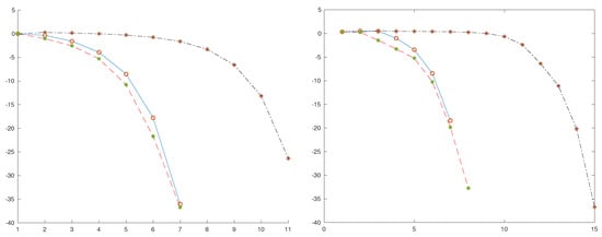
Figure 1.
Logarithms of errors: Newton, blue solid line, red ‘o’; Steffensen, black ‘.-.’, red ‘+’; ASIS, red ‘–’, green ‘*’. Example 1 (scalar) (left); Example 3 (system) (right).
A second example shows the consequences of rescaling the equation. We consider the following.
This function is obtained by the following: . The root of , is times the root of . Hence, Newton’s errors for are one-half the errors of due to the invariance with respect to scales in the variable. The adimensional version of is exactly the same as for and , and the errors of ASIS are also one-half of the errors obtained for . As a consequence, ASIS and Newton’s behave in the same manner as in the first example (ASIS converges faster than Newton’s).
However, Steffensen’s applied to needs 3705 iterations to obtain an error that is less than . We remark that is the initial error. Although it proceeds faster after that (iteration 3716 provides an approximation less than , double precision accuracy), it is clearly an unpractical method in this case. In Figure 2, we show the logarithms of the errors of classic Steffensen’s (not adimensional): In the first 3700 iterations, the errors look similar to a constant, and after that, it behaves as a second-order method. Its region of quadratic convergence is not so small, but it takes a long period to reach it from the initial guess. It can become worse for finer rescalings: The method can blow up due to roundoff errors for for large c. This behavior is normal for Steffensen’s method: its convergence and its speed of convergence, when it converges, depend strongly on the scaling of both the variable and the own function.
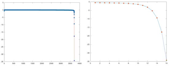
Figure 2.
Example 2: Logarithms of Steffensen’s method for , red solid line, blue ‘*’ (left); iterations from 3700 to 3716, blue solid line, red ‘*’ (right).
The last example in this section is a system of two nonlinear equations with two variables.
This system is obtained from an optimization problem by unrestricted minimization of the following function:
which is the Euclidean norm of a quadratic curve.
Starting from , both Newton and Steffensen converge. As it happens with our first one dimensional equation, Steffensen’s is clearly slower than Newton. Among the possible choices of the divided difference operator, we used the one in [28].
Once again, we try the adimensional version of the system, which is normalized via the Euclidean norm, and we obtain the following:
with the change of the following variables.
The fact that is diagonal simplifies the change of variables (which becomes a diagonal transformation). On the other side, some good features of the original system, such as the symmetry of the gradient, are lost in the adimensional system (therefore, the divided differences operator is no longer quasi-symmetric.
Its behavior is similar to that of the scalar case: ASIS is faster than Newton’s, and Steffensen’s is clearly slower, as observed in Figure 1.
As systems with greater order behave in a similar manner (ASIS is competitive with Newton’s, even sometimes with better performance, and often overcomes stability and convergence problems arising in classic Steffensen’s method), the last example was included as a representative for the sake of simplicity.
However, for really large systems, other issues appear, such as conditioning and dependence among variables and the advantages of ASIS method are not so evident (advantages of Newton’s method are not so evident either). There, ASIS can be a supporting method for solving equations. For instance, the BFGS formula for updating gradients in quasi-Newton methods is a strategy where ASIS improves the performance of the secant method, which is traditionally used in optimization.
The increase in computational cost of ASIS versus classical Steffensen’s is due to the evaluation of preconditioning . As normalization of the adimensional form of F is not necessary, a simpler matrix is used such that is an option. A good choice for B can simplify the problem, as we saw in the square root example in Section 2.2.
8. Conclusions
This paper was motivated by the study of quasi-Newton methods in optimization. It is somehow surprising that despite Steffensen’s method being a well-known method (not as popular as Newton or secant, but well known), which can be implemented without explicit knowledge of derivatives, it is not used or even proposed as a feasible method in this topic. Some insight makes it clear that the weakness of Steffensen’s in scalar equations increases when dealing with equations in several variables. Nevertheless, most of these weaknesses are related to dimensional troubles. Independence from dimensions makes Steffensen’s method (and other methods) more robust and liable.
After some considerations about dimensionality, in this paper, we introduced the adimensional form of functions and polynomials in order to analyze the convergence of iterative methods. These adimensional forms make possible the construction of methods based on classical ones that are adapted from scale dependent methods and overcome all concerns due to dimensionality and scaling. Here, we produced the ASIS method based on the classic Steffensen’s method.
Semilocal conditions are settled in order to ensure convergence of ASIS. The ASIS method has the same convergence conditions as Newton’s method. This is a really interesting result, because, in general, conditions so far are more restrictive for classic Steffensen’s than for Newton’s. The obtained estimates are optimal in the sense that adimensional polynomials reach estimates. This optimality is also an important improvement with respect to other estimators in the literature, which are not optimal. Optimality improves the theoretical region of convergence. In fact, ASIS is at least as fast as Newton’s for polynomials.
These semilocal conditions are not only introduced for theoretical knowledge but also for practical reasons: hybrid methods using different algorithms that slower for the initial iterations with the goal of obtaining approximations into the regions of convergence and faster ones when the approximations are close enough to the exact solution are often devised. In order to obtain good performance, well fitted estimators are needed.
The price to pay in order to obtain adimensional functions is an increase in computational cost due to a change of variable that must be implemented. However, this cost can be reduced because, in general, is not an accurate requirement, although the analysis of softening conditions is outside the scope of this paper. It is remarkable that even random numerical errors do have dimension. Randomness is a numerical condition, but it affects the measure of the parameters.
Finally, we remark that some conditions in the theorems in this paper can be relaxed. Not only the exact evaluation of the inverse of but also the conditions on the second derivative can be relaxed, because it is enough to ask for Lipschitz continuity of the first derivative or some other weaker conditions appearing often in the literature.
Last but not least, ASIS is a good alternative method for quasi-Newton methods in optimization because of its interpolating conditions (no need to evaluate derivatives), robustness, and speed of convergence.
Some features of the method, such as difficulties from ill conditioning, or large systems are actually under research, and the results so far are promising.
The techniques developed here can be extended and generalized to other kind of algorithms (numerical solution of differential and integral equations, regression, interpolation, etc.).
Summing up: although it is often disregraded, dimensional analysis is a powerful tool that helps to improve the performance of algorithms and helps in obtaining a better understanding of their theoretical properties. Adimensional functions rid us of the drawbacks induced by heterogeneous data.
Funding
Funded by ESI International Chair@CEU-UCH, Universidad Cardenal Herrera-CEU.
Acknowledgments
First and foremost, this paper and its author are greatly indebted to the comments, suggestions, and encouragement provided by Antonio Marquina, whose help improved both the paper and the author.
Conflicts of Interest
The author declares no conflict of interest. The funders had no role in the design of the study; in the collection, analyses, or interpretation of data; in the writing of the manuscript, or in the decision to publish the results.
References
- Meinsma, G. Dimensional and scaling analysis. SIAM Rev. 2019, 61, 159–184. [Google Scholar] [CrossRef] [Green Version]
- Buckingham, E. On physically similar systems: Illustrations of the use of dimensional equations. Phys. Rev. 1914, 4, 345–376. [Google Scholar] [CrossRef]
- Potra, F.A. On Q-order and R-order of convergence. J. Optim. Theory Appl. 1989, 63, 415–431. [Google Scholar] [CrossRef]
- Strang, G. Linear Algebra and Learning from Data; Wellesley-Cambridge Press: Wellesley, MA, USA, 2019. [Google Scholar]
- Higham, N.J. Newton’s method for the matrix square root. Math. Comp. 1986, 46, 537–549. [Google Scholar]
- Higham, N.J. Stable iterations for the matrix square root. Numer. Algorithms 1997, 15, 227–242. [Google Scholar] [CrossRef]
- Ortega, J.M.; Rheinboldt, W.C. Iterative Solution of Nonlinear Equations in Several Variables; Academic Press: New York, NY, USA, 1970. [Google Scholar]
- Ostrowski, A.M. Solution of Equations in Euclidean and Banach Spaces, 3rd ed.; Academic Press: New York, NY, USA, 1970. [Google Scholar]
- Kantorovich, L.V.; Akilov, G.P. Functional Analysis in Normed Spaces; Pergamon: New York, NY, USA, 1964. [Google Scholar]
- Dennis, J.E. On the Kantorovich Hypothesis for Newton’s method. SIAM J. Numer. Anal. 1969, 6, 493–507. [Google Scholar] [CrossRef]
- Gragg, W.B.; Tapia, R.A. Optimal error bounds for the Newton-Kantorovich theorem. SIAM J. Numer. Anal. 1974, 11, 10–13. [Google Scholar] [CrossRef]
- Tapia, R.A. The Kantorovich theorem for Newton’s method. Am. Math. Mon. 1971, 78, 389–392. [Google Scholar] [CrossRef]
- Argyros, I.K.; González, D. Extending the applicabiility of Newton’s method for k-Fréchet differentiable operators in Banach spaces. Appl. Math. Comput. 2014, 234, 167–178. [Google Scholar]
- Ezquerro, J.A.; Hernández, M.A. Mild Differentiability Conditions for Newton’s Method in Banach Spaces; BirkhAuser: Basel, Switzerland, 2020. [Google Scholar]
- Ozban, A.Y. Some new variants of Newton’s method. Appl. Math. Lett. 2004, 17, 677–682. [Google Scholar] [CrossRef] [Green Version]
- Weerakoon, S.; Fernando, T.G.I. A variant of Newton’s method with accelerated third order convergence. Appl. Math. Lett. 2000, 13, 87–93. [Google Scholar] [CrossRef]
- Nocedal, J.; Wright, S. Numerical Optimization; Springer: Berlin/Heidelberg, Germany, 2006. [Google Scholar]
- Dembo, R.S.; Eisenstat, S.C.; Steihaug, T. Inexact Newton methods. SIAM J. Numer. Anal. 1982, 19, 400–408. [Google Scholar] [CrossRef]
- Ye, H.; Luo, L.; Zhang, Z. Approximate Newton methods and their local convergence. In Proceedings of the International Conference on Machine Learning, Sydney, Australia, 6–11 August 2017; Volume 70, pp. 3931–3933. [Google Scholar]
- Amat, S.; Busquier, S.; Candela, V. A class of quasi-Newton generalized Steffensen methods on Banach spaces. J. Comp. Appl. Math. 2002, 149, 397–406. [Google Scholar] [CrossRef] [Green Version]
- Argyros, I.K.; Hernández-Verón, M.A.; Rubio, M.J. Convergence of Steffensen’s method for non-differentiable operators. Numer. Algorithms 2017, 75, 229–244. [Google Scholar] [CrossRef]
- Chen, D. On the convergence of a class of generalized steffensen’s iterative procedures and error analysis. Int. J. Comput. Math. 1990, 31, 195–203. [Google Scholar] [CrossRef]
- Jain, P. Steffensen type methods for solving non-linear equations. Appl. Math. Comput. 2007, 194, 527–533. [Google Scholar] [CrossRef]
- Johnson, L.W.; Scholz, D.R. On Steffensen’s method. SIAM J. Numer. Anal. 1968, 5, 296–302. [Google Scholar] [CrossRef]
- Gander, W. On Halley’s iteration method. Am. Math. Mon. 1985, 92, 131–134. [Google Scholar] [CrossRef]
- Candela, V.; Marquina, A. Recurrence relations for rational cubic methods I: The Halley method. Computing 1990, 44, 169–184. [Google Scholar] [CrossRef]
- Candela, V.; Marquina, A. Recurrence relations for rational cubic methods II: The Chebyshev method. Computing 1990, 45, 355–367. [Google Scholar] [CrossRef]
- Potra, F.A.; Ptak, V. Nondiscrete Induction and Iterative Processes; Pitman: Boston, MA, USA, 1984. [Google Scholar]
Publisher’s Note: MDPI stays neutral with regard to jurisdictional claims in published maps and institutional affiliations. |
© 2022 by the author. Licensee MDPI, Basel, Switzerland. This article is an open access article distributed under the terms and conditions of the Creative Commons Attribution (CC BY) license (https://creativecommons.org/licenses/by/4.0/).