1. Introduction
Almost all the time, particular status detection involves taking measurements and comparison against one or several threshold(s). If temperature is the parameter of interest, the periodically measured value will be compared against the threshold(s). This approach is used almost everywhere for triggering situations. Cairns J. [
1] used thresholds in toxicology. Chemicals killing half of the tested organisms were studied. However, the need for other thresholds was also mentioned.
Sorting was another application where thresholds are involved. Estivil-Castro and Wood [
2] were determined to use adaptive thresholds for sorting (an adaptive system use floating thresholds). Demaine, Lopez-Ortiz, and Munro [
3] were concerned about data collection. For data collection, they proposed using union, intersection, and difference determination. Demaine, Lopez-Ortiz, and Munro [
3] considered that complexity is a characteristic of a particular data set. For adaptive sorting, they introduced a framework.
In image processing, Otsu [
4] proposed a method for determining the threshold. Binarizing an image means that the result contains two values, 0 and 255. Pixel values are compared against the threshold. If greater, the pixel becomes 255; if lower, it becomes 0. The threshold has to be determined in such a way that one does not lose the important features in the image. Otsu proposed using the image histogram to compute the optimal threshold.
Hou et al. [
5] proposed a minimum class variance for thresholding as a generalization of the Otsu method, as the latter tends to be biased towards the component with larger class probability/larger class variance. The above-mentioned methods differ in the way they calculate the threshold: average versus absolute distance relative to the class variance. Still, the method fails to determine an ideal threshold for data classification, if the two classes are very different.
A multilevel histogram thresholding method was proposed by Lee and Yang [
6] for multi-region image partitioning. Their method shows various constraints. Cheng et al. [
7] proposed the fuzzy c-partition algorithm for threshold determination. The gray-level image histogram was partitioned into several fuzzy sets using the c-partition algorithm.
An easy-to-understand method for optimal threshold determination in image processing begins with a particular value. Often, the threshold is first set to the average value in the image. The image pixels are split into two sets on the basis of the comparison against this value. Average values are computed for both sets. The next iteration threshold value is the mean of these values. The image is then split again using the result. These steps are to be repeated until the difference between two threshold values is small enough.
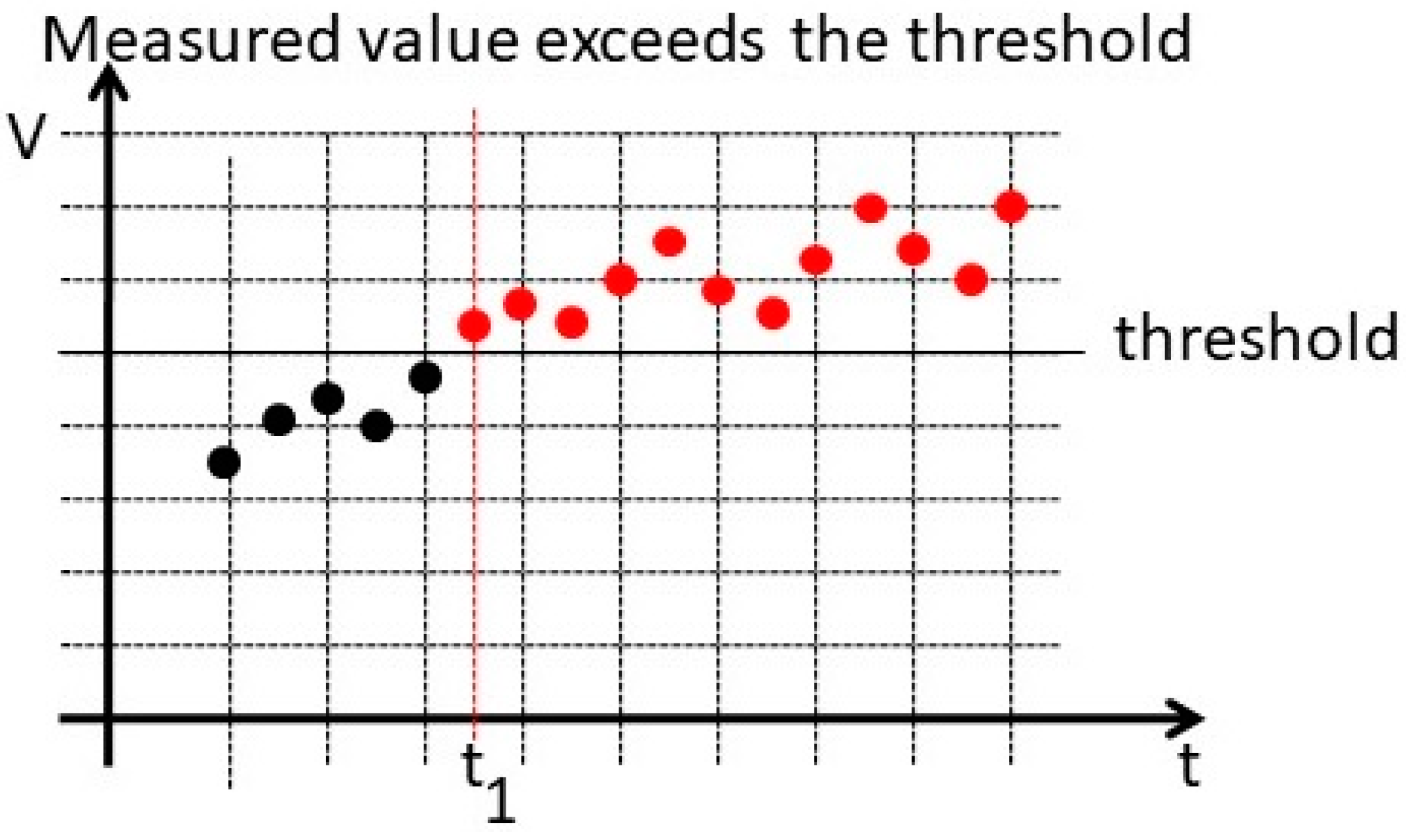
Both measurements and threshold can be seen in
Figure 1. The abscissa denotes the time. The ordinate may represent any value of interest (including percentage). In
Figure 1, the ordinate denotes ‘value’. The measured values exceed the threshold at moment t
1. After exceeding, the system performs signalization. Sometimes a confidence is used. In a possible case, confidence considers the number of values above the threshold (the larger this number, the higher the confidence).
In a heater’s example, if temperature measurements are found to be higher than threshold, the system should stop the heat source and signalize. This is similar to the case depicted in
Figure 1. Before ‘t
1’, the measured values are lower than the threshold. At moment t
1, however, this situation changes. The system can now signalize this status.
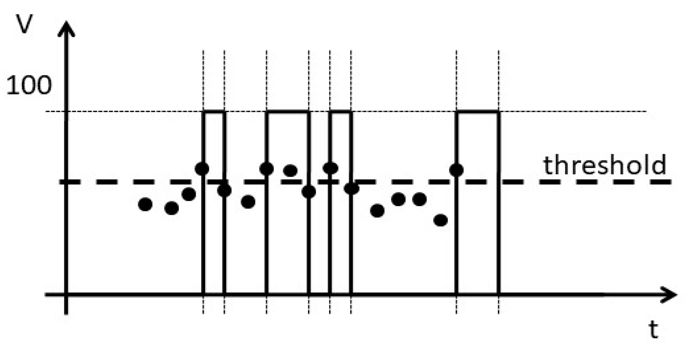
Measurements are usually affected by errors (signals are affected by noise). Ways to minimize the measurement errors are described in the literature. If the threshold is near measured values, the existing noise may cause the system to trigger to the upper threshold state. This can be seen in
Figure 2. Oscillations may occur in such a case, and the system may become unstable. Oscillating behavior is undesired because it can cause system damage.
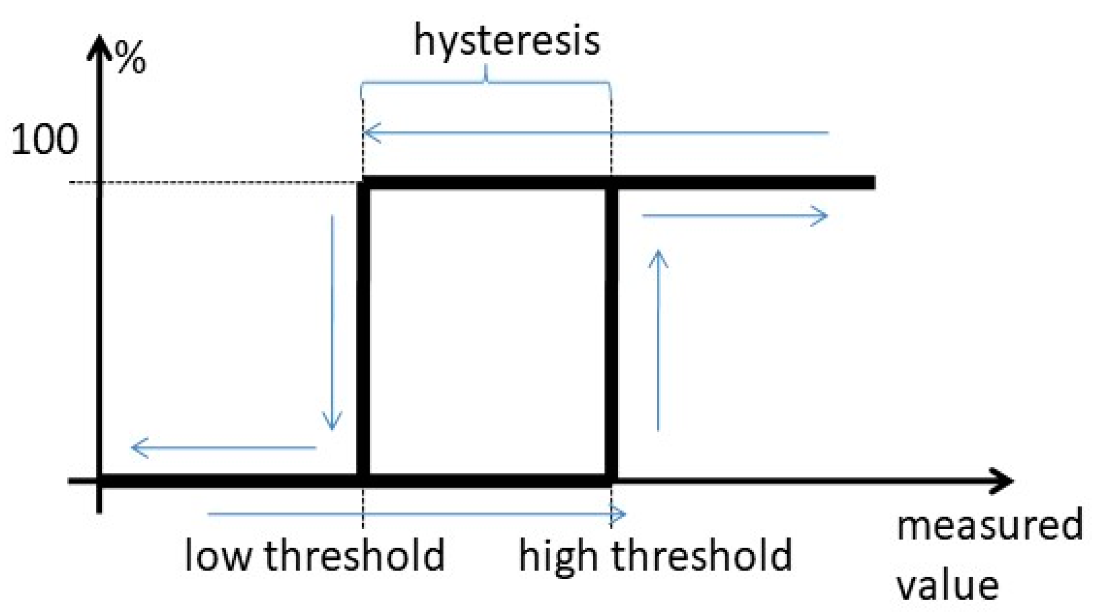
A hysteresis may be used to avoid the problem shown in
Figure 2. Therefore, two thresholds are defined. Increasing measured value will over time exceed the high threshold causing the system to signal a new state. Decreasing values will reach the low threshold and eventually go below it. When this happens, the system will signal it. This situation can be seen in
Figure 3. Using a hysteresis makes the system less sensitive to noise. One may use a value and an offset to compute the two thresholds.
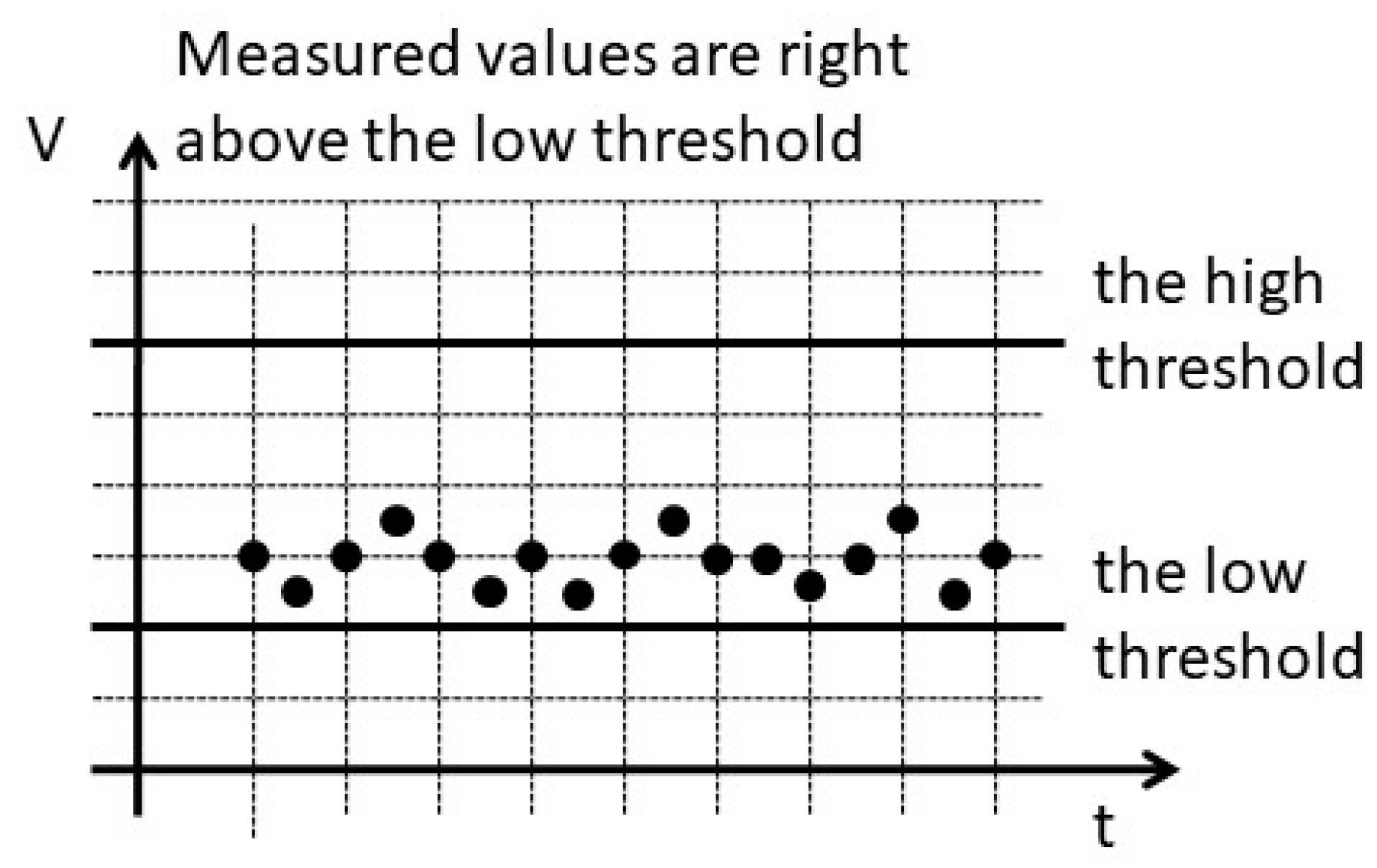
Of particular interest is the case where the measured values are close to the threshold (above or below it). One may say that the values are located in the threshold vicinity. The ‘vicinity’ can be a small interval of 10% of the threshold value. In addition, the vicinity can be application-dependent. Since the threshold is not exceeded, the system cannot detect and signalize a new state.
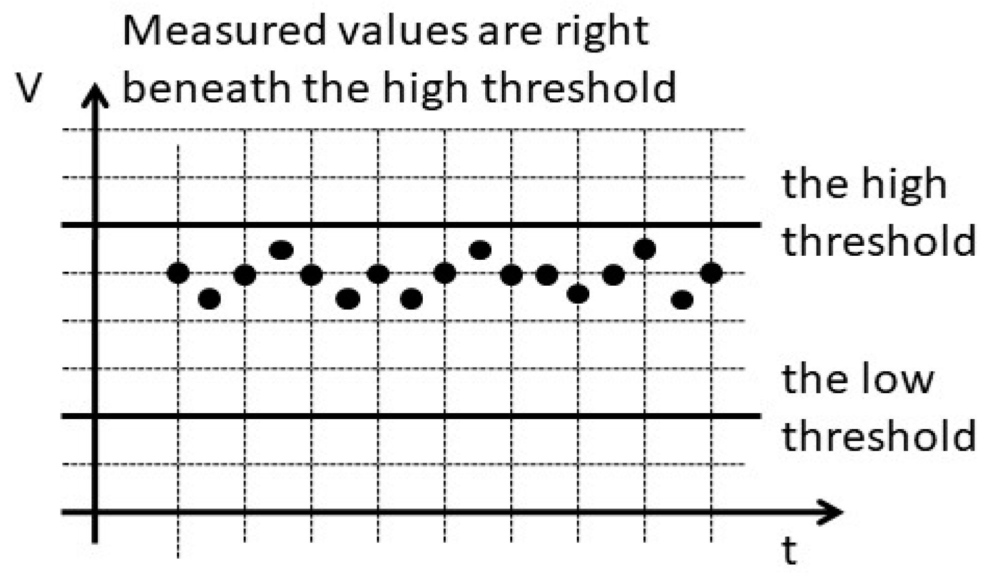
The system may remain in such a situation indefinitely (this occurrence may be caused by the environment, for example, in the automotive domain, the image delivered by the onboard camera is affected by weather such as rain, snow, condensation, etc.). The cases of both thresholds can be seen in
Figure 4 (the values are right above the low threshold) and
Figure 5 (the values are right below the high threshold). Changing threshold values to mitigate this problem does not guarantee that such a situation will no longer occur. It is important to note that there are situations (for example, in computer vision) in which one cannot decide if the system performs correctly by viewing the images/recordings.
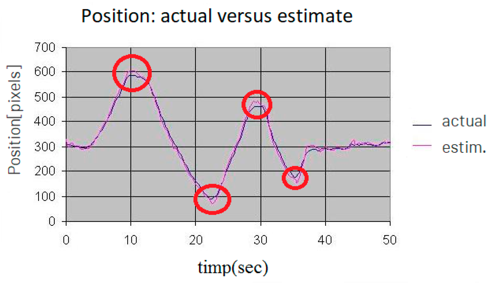
This paper presents one possible way to deal with what is called “the threshold problem”. An estimator will be used to predict the next iteration value. Instead of the measured value, the estimated value will be compared against the threshold. Members of the α–β tracking filter’s family are used to demonstrate the possibility of solving this problem. Although the family filters are tracking reasonably well, the sign-change of the first derivative of the tracked signal causes errors (see local maximums and minimums in
Figure 6). All family filters will be tested in this paper in an attempt to solve this problem. The performance of each filter will be compared with that of others for different threshold values. One such situation was observed in computer vision applications where one could see the image blurriness, but the system did not report it (automotive systems). The experiments are used to assess the performance of each filter in the family in solving the “threshold problem”.
Here, there are certain constraints related to time budget, memory, and real-time operation since this domain uses embedded systems. Since the objective is to address as many computer vision problems as occurring on a certain hardware platform, one shall find and employ the appropriate algorithm that ensures solving the problem and meeting the above demands.
The family filters are introduced in
Section 2. There are a total of three filters in this family: α–β (the simplest), α–β–γ, respectively, α–β–γ–δ (the most complicated one). The problem is that the filters are not inherent stable for all combinations of filters’ parameters (α, β, γ, and δ). For a more concise presentation, stability is studied just for the α–β–γ filter whereas the stability conditions are formulated for both α–β–γ and the α–β–γ–δ filters.
Section 3 discusses the experiments to assess each filter’s performance. Their abilities are discussed in
Section 4 where some conclusions are also presented.
2. The Alpha-Beta Family of Filters
Tracking filters are an important aspect of target tracking, as they help reduce tracking errors and make accurate estimates. During the Cold War period, Sklansky [
8] created the α–β family of filters. The α-β family of filters, which are Kalman equivalent constant state filters for tracking constant velocity and constant acceleration targets, are limited in their ability to accurately track a high-momentum maneuvering target which is characterized by a jerky motion.
In recent decades, several techniques have been proposed in an attempt to create filtering equations that are used to model the constant jerk.
Discrete data are widely used in air traffic control, missile interceptions, antisubmarine warfare, and other applications to forecast the kinematics of moving objects. They were designed to estimate velocity and position and also to operate in radar tracking, based on noisy (measurement) data. Three members of this family have been applied not only to make predictions, but also for tracking, comparable to the Kalman filter [
9,
10,
11,
12,
13]. They have been used by Kalata and Murphy [
14] to track rate fluctuations and make predictions. The tracking parameters were also a topic of interest for Kalata [
15]. Tenne and Singh [
16] have presented approaches to improve the efficiency of the filter family. Their work also showed how to develop stable α–β filters. Furthermore, α–β–γ filter has been applied in computer vision applications. The filter performance was compared with Kalman’s by Corke and Good [
17]. They have noted that Kalman’s coefficients converge to nearly constant levels, and for this reason, computing them is inefficient. In this situation, the α–β–γ filter produced results that were comparable to Kalman’s but required less computational work. These filters have also been implemented by Stanciu and Oh [
18] to predict the location of the target within the image plane. For each iteration, the target position was captured and the data was put into a α–β–γ filter, which predicted the location one step forward. Tracking performance is greatly enhanced by this information.
Stanciu and Molnar-Matei [
19] also performed a performance comparison between the α–β–γ filter and the Kalman filter. The authors have managed to find values for the filter parameters that prove better performance than Kalman.
Ng, Yeong, Su, and Wong [
20] presented the α–β–γ filter for motor position control using the cascaded Proportional Integrative Derivative (PID) law. They have developed a new, more precise, design procedure for the α–β filters.
Recently, Lee et al. [
21] proposed using a genetic algorithm to find the best parameter values of the α–β–γ filters. Their results indicated a performance improvement while the noise was kept at acceptable levels.
Wu, Chang, and Chu [
22] presented an ideal design of the α–β–γ–δ filter to increase the tracking accuracy of what is known as the third order filter’ (which is actually the α–β–γ–δ filter). The third temporal derivative of the value of interest (known as the ‘jerk’) is the added value. On the other hand, this tracking filter can anticipate the second-order derivative of the value of interest. The authors claimed that the accuracy of the tracking has improved significantly.
The α–β filter was used to smoothen the target trajectory [
23]. The authors use what they call “steady state conditions for Kalman smoother” to derive an alpha-beta smoother. Despite the suboptimal estimate, the simplicity of the filter makes it attractive in many applications.
An α–β–γ filter was also proposed to suppress the so-called ‘sea clutter’ [
24]. Robust sea-target detection (especially low-observable ones) is affected by this phenomenon. The authors mentioned that sea clutter can vary with polarization mode, frequency, and other factors, which may significantly limit the radar detection capability. Instead of modeling sea clutter, the authors employ the α–β–γ filter to separate it from the targets. Their experiments showed promising results.
Kosuge [
25] is concerned with deriving an α–β filter using the steady-state variance of the estimated velocity for a target. The product of the velocity variance and the nth power of the steady-state estimated error is used for this purpose. A mathematical expression to compute steady-state velocity error for moving targets with constant acceleration was derived.
The problem of tracking the target is addressed in [
26]. Their tracker uses a cloud model, an α–β filter, and a rule bank to accurately track maneuvering targets. The authors mentioned that the experiments performed showed satisfactory results.
The design of a high-performance α–β filter was the concern of Ting-En Lee et al. [
27]. Starting from the observation that the filter’s estimation performance is dependent on the parameter values, they combined the fuzzy logic with what they called “evolutionary optimization” to determine the best estimation filter. The determined filter was able to accurately track the signals and also reduce noise.
Ying-Qing et al. [
28] used the α–β filter for image stabilization (motion compensation). Interframe global motion vectors were predicted to compensate for the motion. Constant velocity motions were considered for compensation. The experimentally obtained results revealed that high-frequency dithering can be mitigated using the tracking filters of this family.
Bo Li [
29] combines the α-β filter with the Back Propagation Neural Network (BPNN) to track the target. The adaptive α-β filter is used to compute the region of optimal parameters. The net effect is a region reduction. The result is fed to the BPNN, allowing for accurate recognition. The work focused on efficiency and reliability. Various scenes were used for testing. The author indicates a significant improvement obtained with this method.
Khan et al. [
30], introduced what they called the “new learning to the prediction model”. The main idea was that once the filter parameters are established, they remain constant. Therefore, tuning them according to the historical values leads to higher performance. Their method aims to improve the performance of the prediction algorithm in dynamic circumstances. The α-β filter and the Deep Extreme Learning Machine (DELM) algorithm were employed by the authors. The method was referred to as “learning to alpha-beta filter”. There are two main components: a prediction part and a learning part.
Murzova and Farber [
31] are concerned with tracking maneuvering objects using the linear frequency modulated waveform (LFM). The range-Doppler coupling of LFM waveform can increase but also decrease the tracking accuracy. It is also mentioned that an α-β filter can reveal an estimation lag error. Therefore, an optimal relation between the filter parameters α and β is important to improve the tracking of the target. Such a relationship would determine the minimum value of total variance.
There are three filters in the α–β family. All of them work in two steps: prediction and correction. Since they are not stable by default, the stability is studied for the two more complex filters in the family. All three filters were implemented and tested to compare the results with each other. The filters and the results obtained are described in the following sections.
2.1. The Alpha-Beta Filter
This is the simplest filter in the family. It estimates the “next iteration’s value” for the variable “
x”. The prediction step is expressed mathematically by Equation by Equation (1):
In Equation (1), the denotes the predicted value for iteration k + 1, the denotes the “smoothed” value for iteration k, and the and designates the smoothed value of the first and the second derivatives for iteration k. It is important to note that x can be any variable of interest (distance, pressure, voltage, etc.). T represents the sampling time interval. The estimated value and its first derivative are corrected (smoothed) in the second step.
The correction (smoothing) is given by Equations (2) and (3):
The estimated value and its first derivative are corrected (smoothed) in the second step (for the current iteration) once the variable’s value is being measured (“observed”). In Equation (2), the variable value is corrected by adding to the already computed prediction a fraction (represented by the alpha parameter) of the difference between the observed value and the predicted one. In Equation (3), the first derivative’s value, denoted by is also smoothed in the same manner. However, this time, the weighting factor is .
2.2. The Alpha-Beta-Gamma Filter
The second family member is the alpha-beta-gamma filter. Unlike the first one, this algorithm predicts the first’s derivative value as well. The filter estimates the first derivative of the value and the next value iteration in the prediction step. When the estimated values are known, they are smoothened (adjusted) in the second step. (4) and (5) actually represent the estimation step. In Equation (4), the predicted value for iteration
k + 1 is denoted by
, the
represents the corrected value for iteration
k, while the corrected value of the first derivative for iteration
k is denoted by
and the sampling time is represented by the letter
T.
In Equations (4) and (5), the denotes the smoothed value of the second derivative for iteration k (the rest of the notations remaining the same).
Correction (smoothing) is given by Equations (6)–(8) and takes place in a manner similar to that of the previous filter. Both the variable and its first derivative are smoothed. The estimated value and its first derivative are corrected (smoothed) in the second step.
The Alpha-Beta-Gamma Filter Stability
As mentioned above, a stability study is performed for this filter. Although all members of the α–β family were tested, stability was studied only for the α–β–γ and α–β–γ–δ filters (in order to be of any use, this must be considered). The Jury stability criterion is employed to this purpose. In fact, the filter parameters must meet certain conditions for a stable algorithm.
To study the stability, one must obtain the filter transfer function. The so-called Z-Transform will be applied to determine the transfer function. As such, the prediction equations shall become as shown in Equations (9) and (10):
The correction is expressed mathematically in Equations (11)–(13). In Equation (13), the term
considers that
is the former value of acceleration. Finally, the filter transfer function is given by Equation (14):
As mentioned above, the predicted value (referred to as target’s ‘position’) can be any measurement of interest (distance, height, pressure, etc.) with sensor values being used to calculate estimations. Another transfer function that relates the predicted ‘velocity’ to the observed position can also be derived for the filter.
A criterion is needed to examine the stability of the filter. Jury’s criterion is used to study the filter’s stability. The study is presented for the α–β–γ only (since it will be performed in the same way for the others).
The Routh–Hurwitz stability criterion cannot be directly implemented in the
z-plane because its boundary differs from that of the s-plane [
32]. The Jury stability test, on the other hand, is a similar procedure for discrete systems. Consider the following Equation (15):
The Jury stability test is formed as shown in
Table 1.
The Jury stability criterion contains one row for a second-order system examined. With each additional increase of system’s order, two more rows are added to this table (even number rows have the same elements as previous ones but arranged in reverse order). The odd-numbered rows have the elements defined as can be seen in Equations (16) and (17):
The polynomial G(z) defined by (18) and (19) has no roots outside the unit circle (or on its border) if the following
n − 1 constraints are satisfied [
32]. The conditions expressed by (20) and (21) are sometimes called “necessary stability conditions”. Conditions expressed in (20)–(22) are sometimes referred to as “sufficient stability conditions”.
The characteristic polynomial coefficients for the filter position can be seen in
Table 2.
This is used in the following section to study the stability of the filter.
The first necessary stability condition is then:
Expression (23) restricts the parameter
γ to positive values. The second necessary stability condition is represented by Equation (24):
There are two sufficient stability conditions for the filter stability. Since the parameter
of the filter is 1, Equation (20) translates into (25):
Equation (25) will lead to (26):
The second condition is expressed by Equation (27):
Since the parameter α is always positive and the (α − 2) is also negative (according to Equation (26), the Expression (27) transforms as shown in (28):
Expression (28) leads to a constraint for the parameter γ shown (29).
Based on this stability criterion, the equations that the filter’s parameters must satisfy are given by Equations (23), (26) and (29) The values of the filter family parameters are chosen to satisfy the above test of the functionality and stability of the filter. As such, the parameters values were α = 0.75, β = 0.8, γ = 0.25, and δ = 0.70. The filters can be implemented in many software packages (MATLAB R 2014, Excel v.16.0.1, etc.).
2.3. The Alpha-Beta-Gamma-Delta Filter
The α–β–γ–δ filter uses an additional equation to predict the second derivative of the value of interest (commonly known as ‘acceleration’). Similarly to the other family members, it works in two steps. Its prediction equations are (30)–(32). In these equations, the term
is called the “jerk”.
There are four correction Equations (33)–(36).
The Jury stability criterion leads to the conditions expressed by Equations (37)–(40).
3. Experiments with These Filters and Results
Since these filters exhibit errors when the first derivative of data changes sign (at local extremes), the proposed method works even when the data are above the threshold (in case of hysteresis, there are two thresholds). It is also worth mentioning that one may choose to use this method when the average value of the data is ‘in a vicinity’ of the threshold. In such a case, the filter is not called or used all the time. The number of required iterations used to compute the so-called ‘average data value’ may depend on the application. The measurement of the distance between the average data value and the threshold is the difference between them.
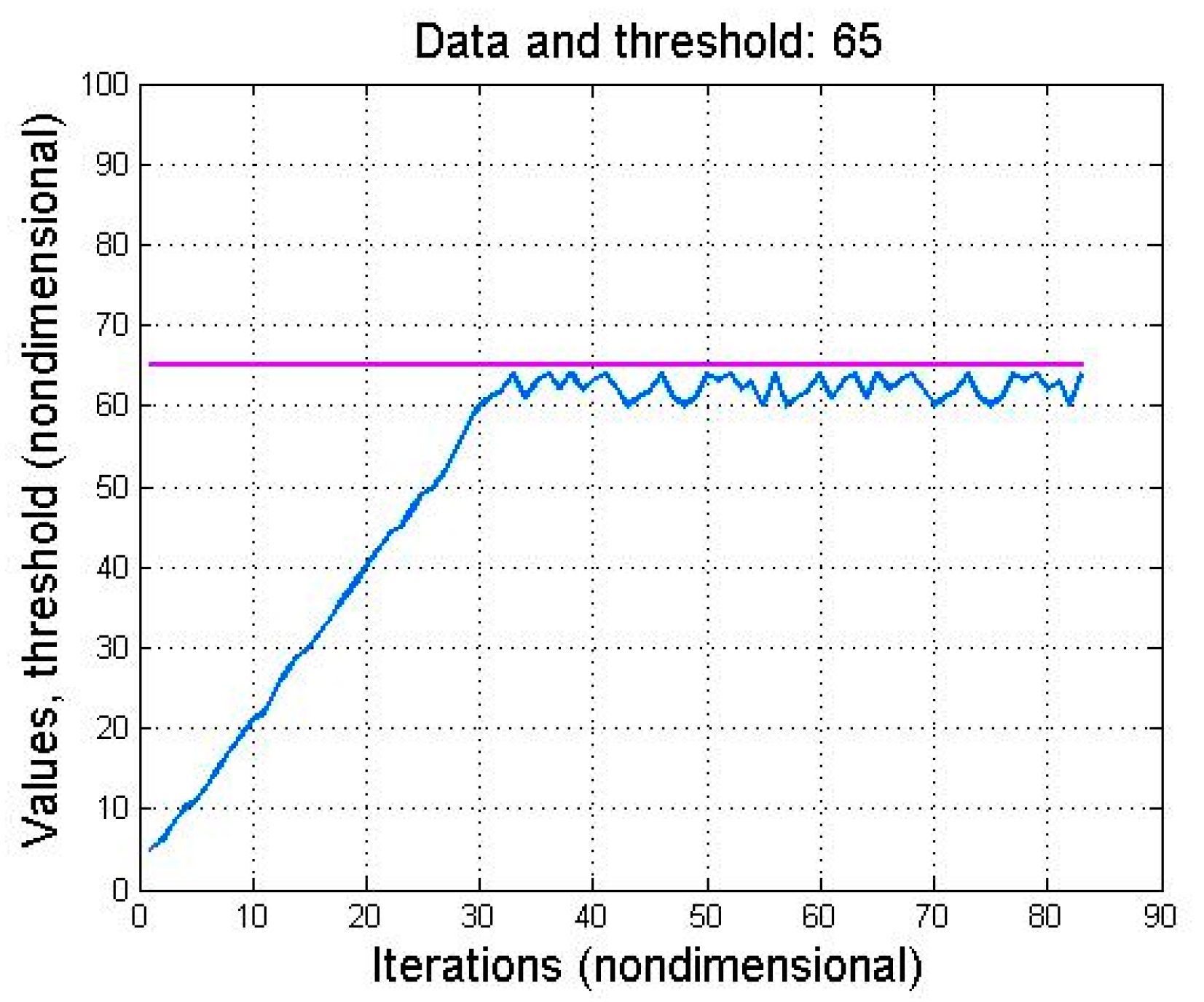
The experiments focused on proving the solution of threshold problems and comparing the performance of the three filters in the α–β family. A set of data was created in which the values slowly increase towards the threshold for testing purposes (
Figure 7). It can be seen that after iteration (temporal step) 30, the data values are right below the threshold.
Several experiments were considered. They determine the iteration in which the estimation exceeds the threshold for the first time for certain (fixed) filter parameters. These results are compared for the three family filters.
The second experiment considers several cases of different ‘distance’ between the threshold and the average data values. For the same data sequence, several thresholds are used with all family filters. The results obtained are compared against each other.
In the third experiment, the filter parameters are adjusted to determine if its estimation can exceed the threshold faster or if the filter works in the case of a larger distance between the threshold and the average data values.
3.1. Experiment I
This (threshold) value was set to 65 for this experiment. Taking into account only data values located in its vicinity (which is the interval between 90% and 100% of the threshold), their average is 62.24. As such, the difference (distance) between the threshold and the average value of the data located in the vicinity of the threshold is 2.759.
The α–β filter is used first. In the first experiment, this α–β filter was used to prove that this family produces the estimated result (a workable algorithm). Since the experiment does not target stability issues, the input (measured) data values slowly increase towards the threshold but remain below it (
Figure 7). The values of the filter parameters were set to α = 0.75 and β = 0.8. Both values lie within the stability intervals (as such, the filter is stable). In the threshold problem, the α–β filter provides an estimate that exceeds the threshold at iteration 33 (as it can be seen in
Figure 8), therefore, sidestepping the problem.
However, it can be observed that there are iterations in which the filter’s estimated values do not exceed the threshold. Therefore, it is interesting to determine the filter performance when the average data are further away from the threshold. However, it is important to determine how other filters in the family behave under the same conditions.
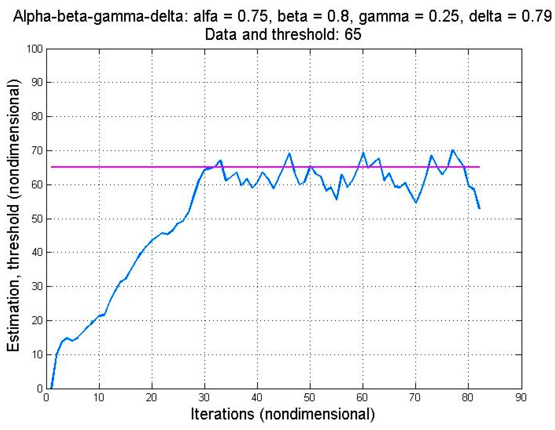
The α–β–γ filter was the second algorithm used to solve the threshold problem. The values of the chosen parameters were α = 0.75, β = 0.8, γ = 0.25. Just like the first filter, the α–β–γ estimation first exceeds the threshold at iteration 33. Unlike the α–β, this filter also provides estimate values that exceed the threshold between iterations 30 and 80 (
Figure 9).
The third algorithm tested under the same conditions was the α–β–γ–δ filter. The parameter values used are α = 0.75, β = 0.8, γ = 0.25, and δ = 0.7. The results can be seen in
Figure 10. Similarly to the first two family members, the α–β–γ–δ filter delivers many estimation values that exceed the threshold. The first such value is at iteration 33. While the α–β–γ filter also does that, the α–β–γ–δ provide larger estimates. This behavior suggests a working filter, even if the “distance” between the threshold and the average data values increases.
3.2. Experiment II
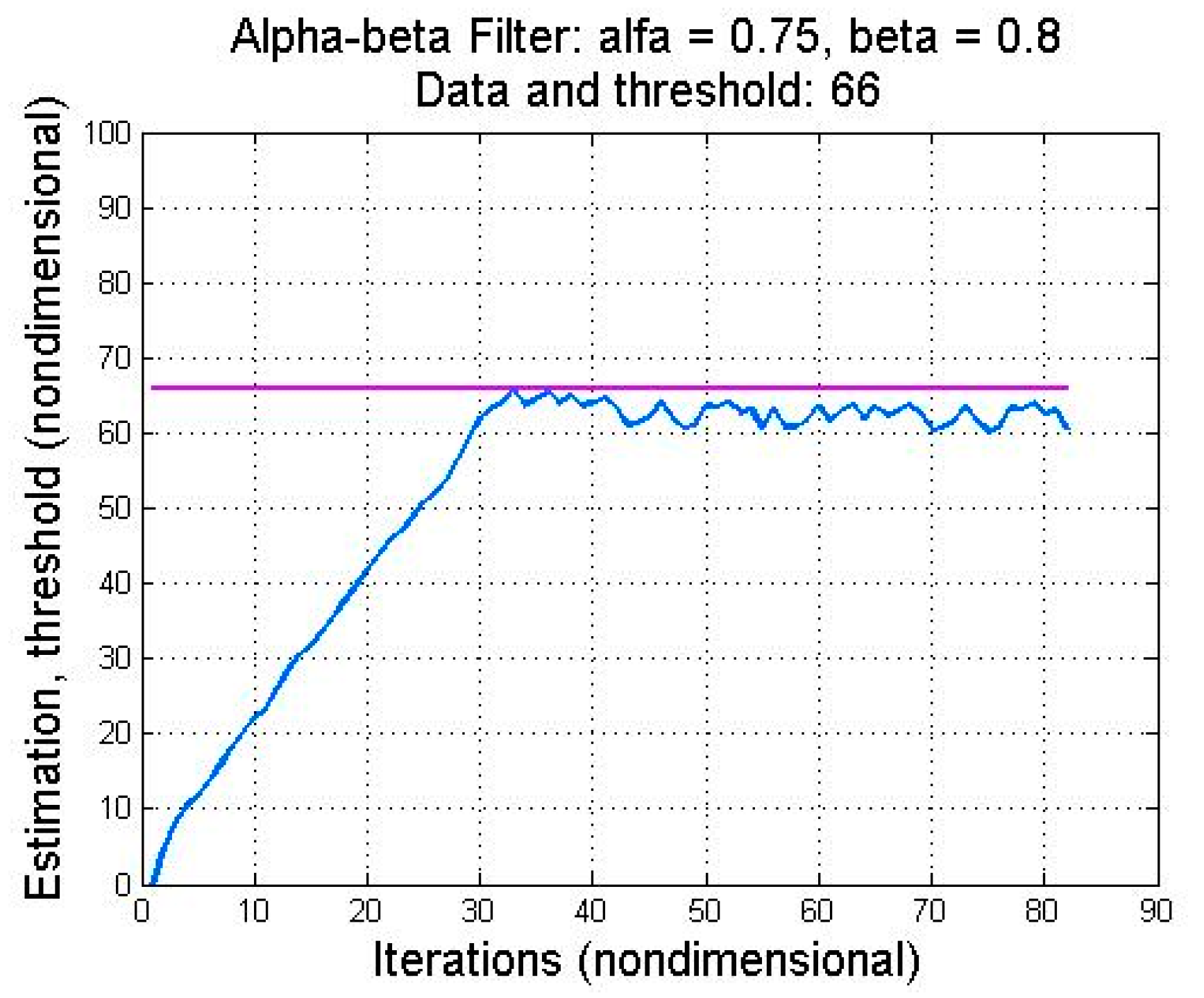
As mentioned above, it is interesting to determine how the filters solve the problem in case of an increase of “distance” between the average data and the threshold. Therefore, a threshold value of 66 is chosen with the same data for all filters. The average value of the data located in the vicinity is now 62.1875 with a distance-to-threshold value of 3.8125. All family filters (having the same parameter values as in the first experiment) were tested in an attempt to determine if they solve the problem. The results of the α–β filter can be seen in
Figure 11.
As can be seen, this algorithm cannot provide an estimate that exceeds this threshold value. Therefore, the α–β filter is not able to solve the problem in this case. It is not expected to work for a further distance increase.
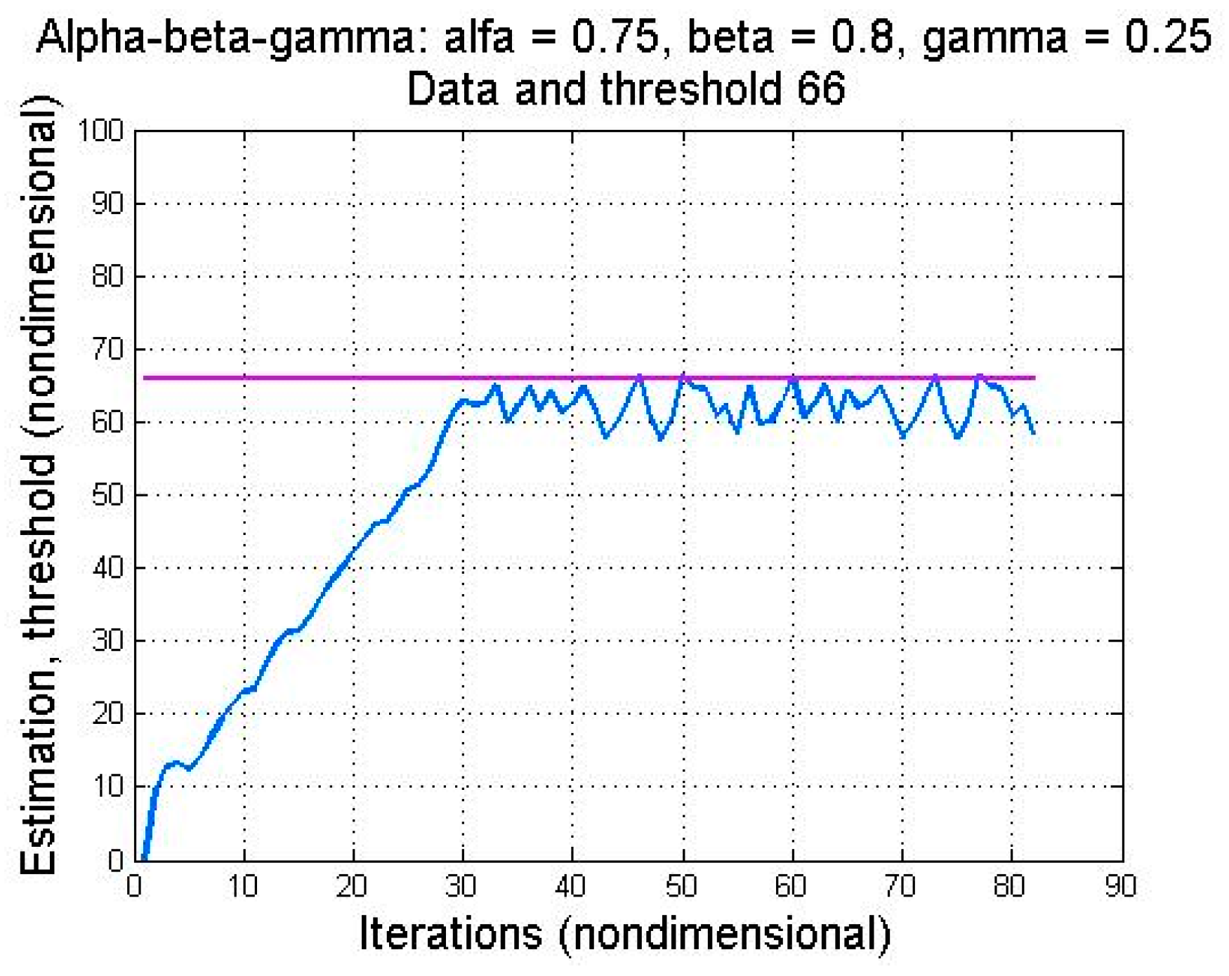
The α–β–γ filter was also used for this threshold value. The results can be seen in
Figure 12. The filter can still deliver several estimate values that exceed the threshold value of 66. The first estimate value that exceeds it is at iteration 46. As such, the algorithm takes more time to solve this problem than in the first experiment.
The last family filter was also tested for this threshold value. The results can be seen in
Figure 13. As can be seen in
Figure 13, the α–β–γ–δ filter delivers many estimate values that exceed thresholds. In addition, the first one is still at iterations 33, despite an increased threshold value. As such, this algorithm works faster than the α–β–γ filter (the first estimate exceeding the threshold occurs in iteration 46).
3.3. Experiment III
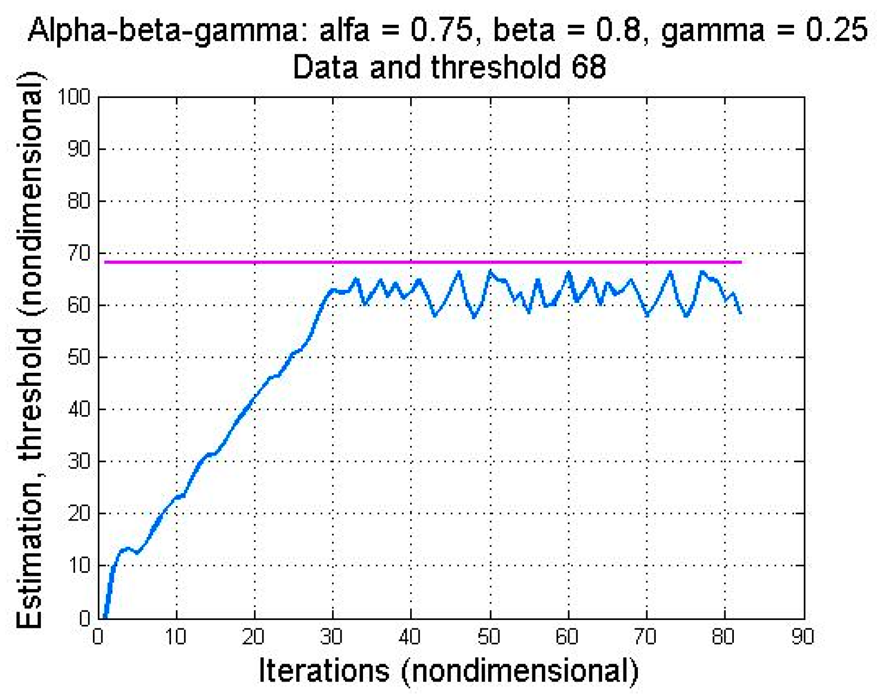
In this experiment, the threshold value was increased to 68. Since the α–β filter was not able to solve the problem for a threshold value of 66, it will not be tested in this experiment.
The average value in the vicinity of the threshold is 63.1428. Therefore, the distance from the actual threshold value (68) is now 4.8571. The first to be tested is the α–β–γ filter. The results can be seen in
Figure 14. As can be seen, the α–β–γ filter no longer delivers an estimate capable of exceeding this threshold value; therefore, it no longer offers a solution to this problem.
The same threshold value was used for the α–β–γ–δ filter. The results can be seen in
Figure 15. The algorithm provides several estimations that exceed this threshold value. As such, the α–β–γ–δ filter is working for the threshold value of 68.
If its performance is compared for threshold values of 66 (
Figure 13) and 68 (
Figure 15), one can see that in the latter, the filters take longer to deliver an estimate exceeding the threshold (iteration 46). Furthermore, there are several times when the algorithm’s estimation exceeds this threshold value. Therefore, it is appreciated that this filter works well under these conditions. In conclusion, the only filter capable of solving the threshold problem (the parameters values were not modified so far) in this case is the α–β–γ–δ. In the following experiment, the threshold value was raised to 70.
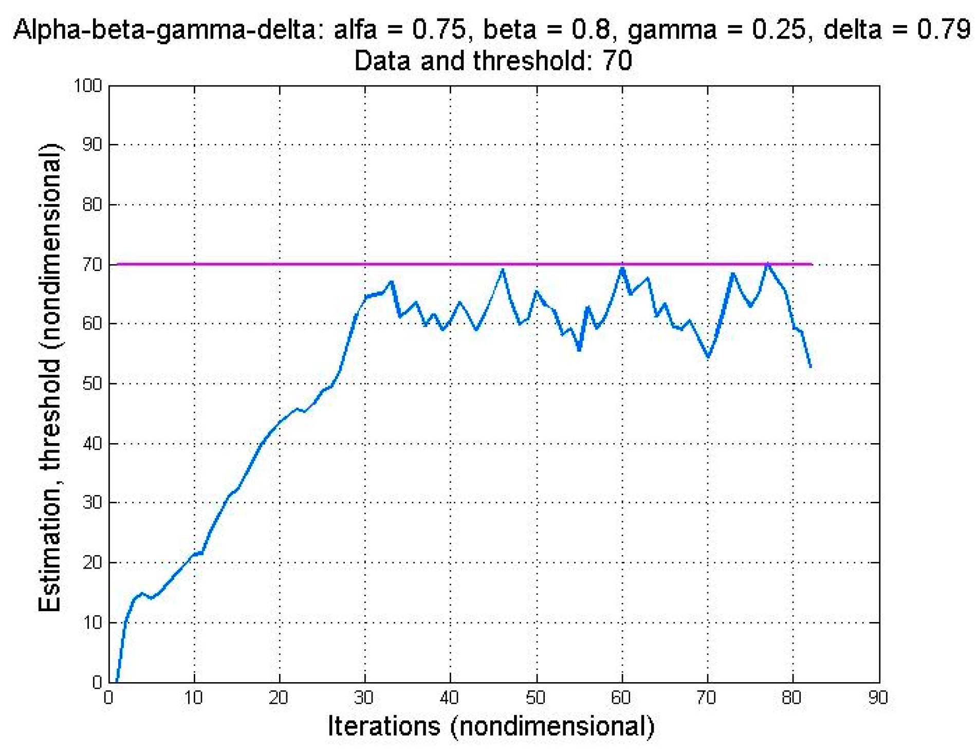
3.4. Experiment IV
The previous experiments reveal the fact that as the threshold to average data value increases, the filters take longer time to deliver an estimate exceeding the threshold or even fail to do that. As the filter’s simplicity increases, they perform better in solving the threshold problem.
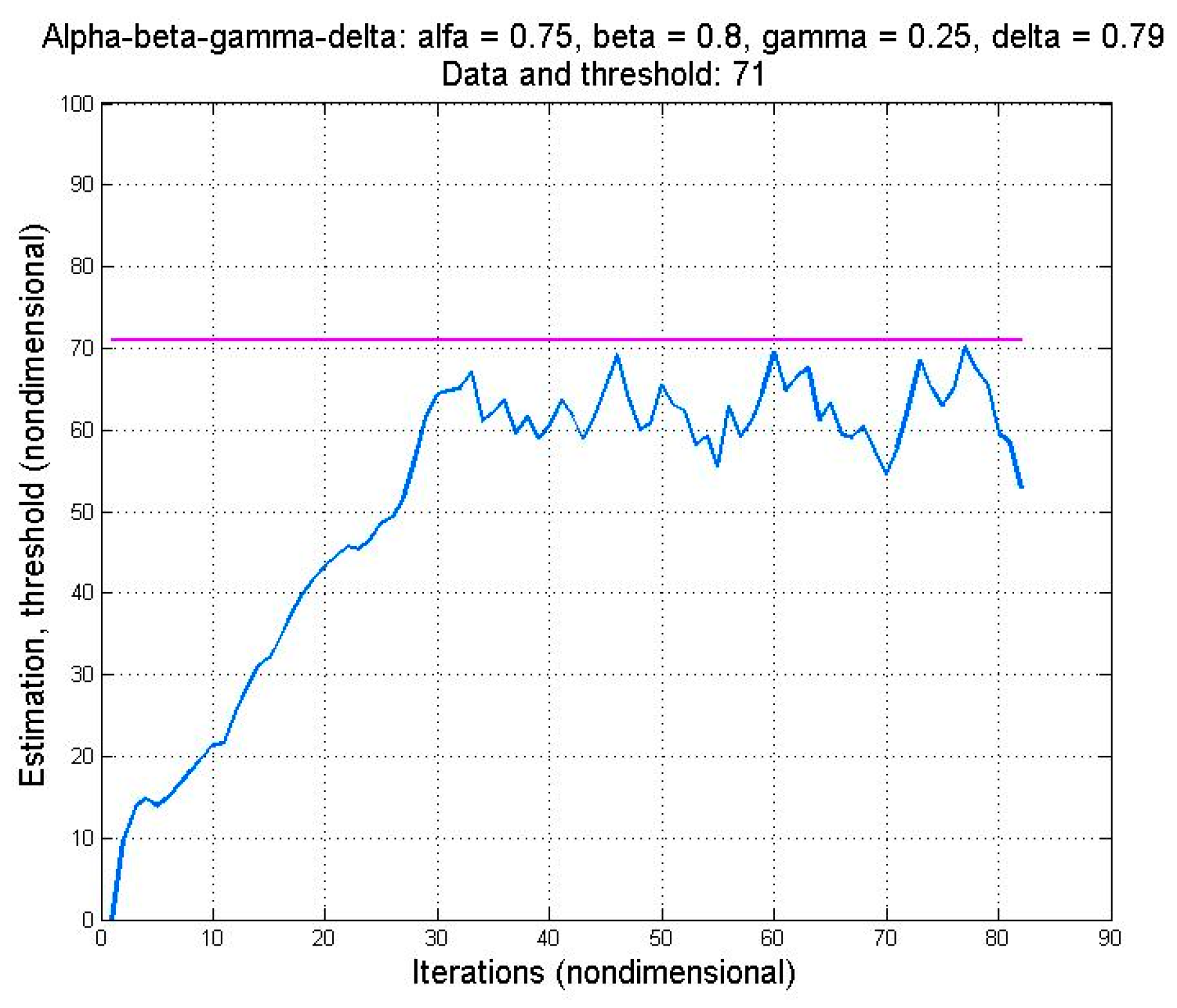
In an attempt to determine the limit to which the α–β–γ–δ filter is able to work even further, the threshold was increased to 70. The average value of the data in the vicinity of the threshold was 64. Therefore, the distance to the threshold was 6. The results can be seen in
Figure 16.
It is important to mention that it takes significantly longer to deliver an estimate that exceeds the threshold (at iteration 77). In addition, the filter delivers only one estimate of this kind. This behavior suggests a marginally working filter in this case; therefore, even a very small increase of the threshold value may reveal a non-working filter. In the next experiment, the threshold is increased to 71.
3.5. Experiment V
To prove that the α–β–γ–δ filter works marginally in the previous case, the threshold was increased to 71. In this case, the average value of the data are located near the threshold is 64. Therefore, the distance to the threshold value is 7.
The results can be seen in
Figure 17. As can be seen, the filter is no longer able to deliver an exceeding-the-threshold estimation for this threshold value.
The performance results found in the above experiments can be summarized in
Table 3. As can be seen here, the α–β filter works only in the first case in which the distance between the average data value located in the threshold and the threshold value is small (2.759). The α–β–γ filter works in the first two cases in which the distance between the threshold and the average data value located in the vicinity of the threshold is 2.759 and 3.8125. The α–β–γ–δ filter works in four out of five cases. This makes this algorithm more suitable than others to solve the threshold problem.
3.6. Experiment VI
So far, five experiments have been carried out in an attempt to classify the three filters in the α–β family. As more complicated algorithms were tested, the value of common parameters did not change (the value of the α parameter remained the same).
One more experiment attempts to increase the performance of these algorithms. Specifically, the parameter values are modified for this purpose. Since it balances performance with computation cost, the α–β–γ filter is chosen for this purpose. The results are tested against those obtained by the same filter but with different parameters. The new parameter values are α = 0.75, β = 2, γ = 1.5. With these parameters, the filter can provide an estimate greater than a threshold of 72 (
Figure 18). Still, it can be seen that the amount of noise introduced has increased.
3.7. Experiment VII
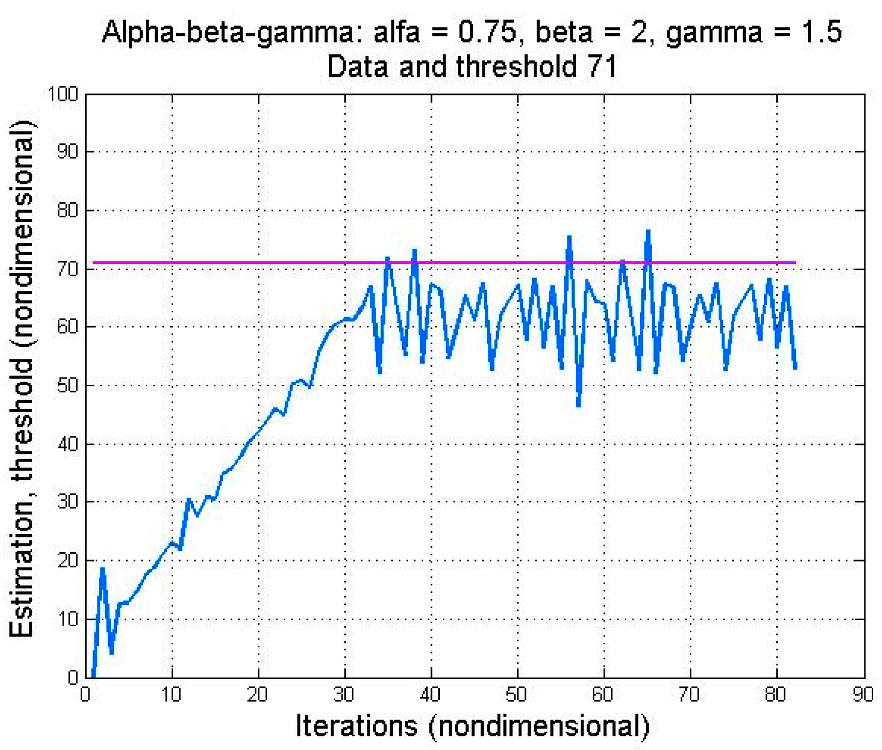
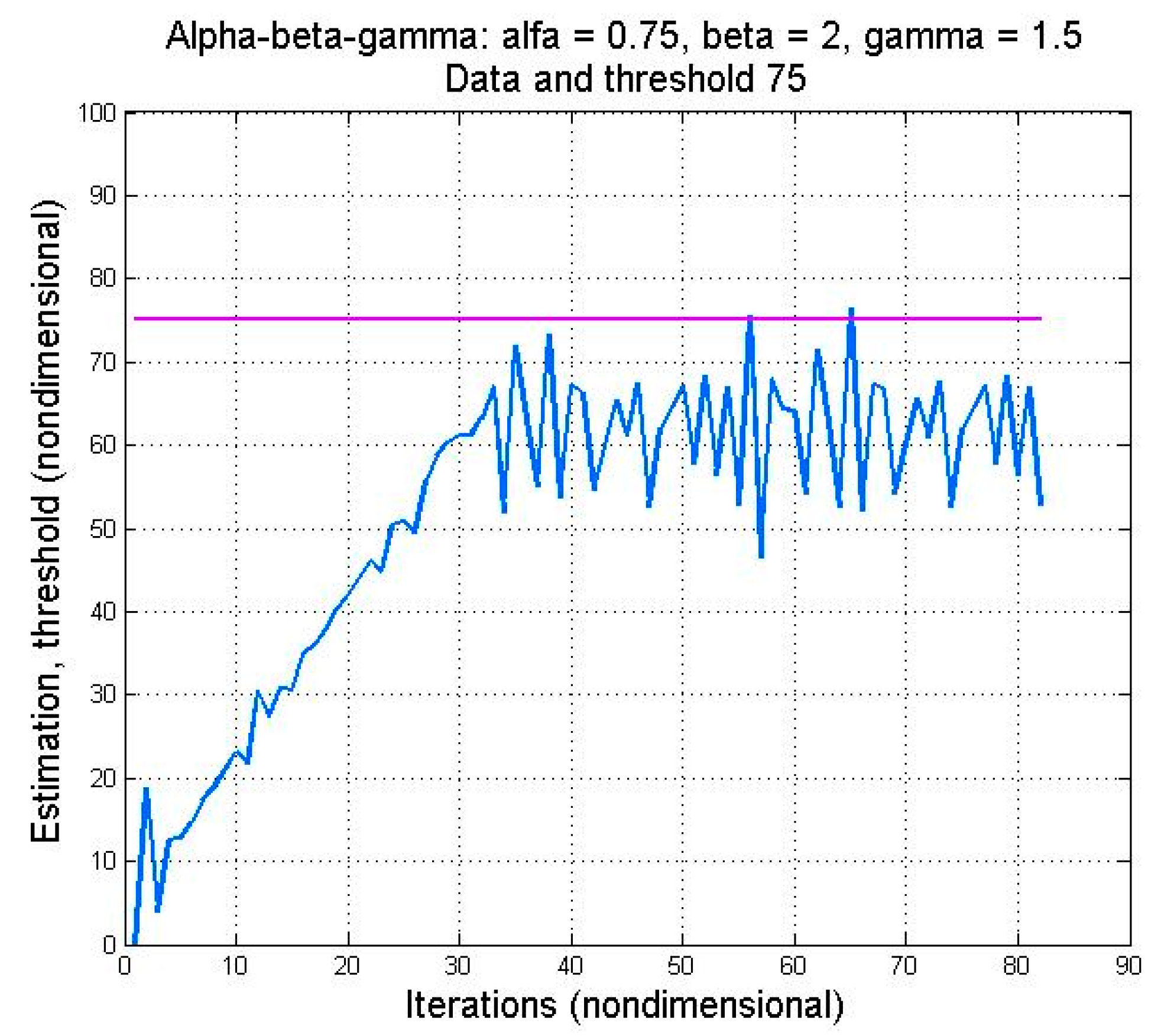
With the first values chosen, the α–β–γ filter was unable to provide an estimate that exceeded a threshold of 68. With the values of the second parameter set, the filter solves this problem even for a threshold of 75. Naturally, it takes longer and the amount of noise introduced has increased.
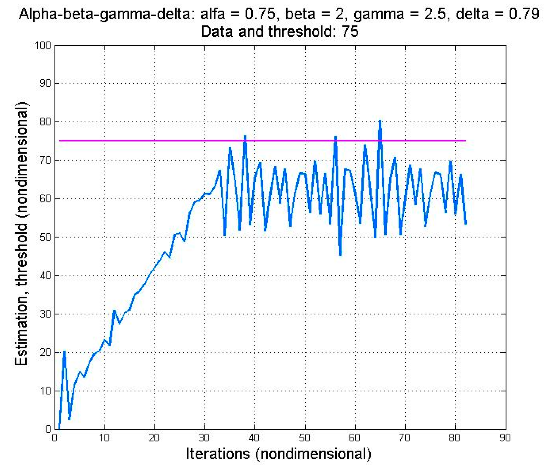
It is now interesting to determine whether the α–β–γ–δ filter works faster than the α–β–γ for this threshold value. The parameters α, β, and γ were set to α = 0.75, β = 2, γ = 1.5, while the last parameter was not changed. The results can be seen in
Figure 19 and
Figure 20. The α–β–γ–δ filter provides an estimate that exceeds the threshold faster (iteration 38) than the α–β–γ for which the first estimate that exceeds the threshold is at iteration 57. However, the amount of noise introduced may not be suitable for all applications.
4. Discussion and Conclusions
The so-called ‘threshold problem’ is defined as a case where the measured data are located close to the threshold but not exceeding it. All three members of the α–β family of filters were tested for increasing data-to-threshold distance to determine if they can solve this problem. This situation was observed in a computer vision application. One does not always make the right decision in such a situation.
As shown above, filters can sidestep the threshold problem for different threshold values. However, this occurs at the expense of a certain amount of noise introduced. It is important to mention that the noise introduced may affect the stability of the system, so one must take that into account.
When a specific amount of data (i.e., the number of iterations) is near the threshold to activate a filter call, one method to reduce noise effects is to utilize filters. The amount of data near the threshold can be defined as a parameter and can vary depending on the application.
Several experiments were performed for several different threshold values with the same data set. As the threshold increased, the simple algorithms failed one after another (starting with simpler towards the more complex algorithms) to solve the problem. These results are summarized in
Table 3. Parameter modification was considered after the most complicated filter was not able to solve the threshold problem.
The α–β, the α–β–γ, and the α–β–γ–δ filters were used in the above work and their results were compared. The results reveal that the α–β–γ–δ filter performs best at the expense of complexity.
The medium complexity (α–β–γ) filter was chosen for an experiment to attempt to increase its performance by tuning its parameters. It delivers a result at the expense of an increased introduced noise. The behavior of this filter was compared with the α–β–γ–δ filter with modified values. However, it also introduced noise.
The proposed method was required to meet the tight constrains (real-time response, memory, power consumption) found in typical automotive embedded systems. It was implemented and tested and showed advantages over the more computational demanding solutions.
Future work is related to specific challenges. One of them is to easily tune the sensibility of an algorithm. In the most basic situation, the algorithm may be sensible, medium-weight, and robust.
It is interesting to see what happens when a particular amount of noise is added (by the selected filter) and to design a framework that helps to determine the ideal filter to be used, depending on the triggering time and the added amount of noise.
It is also intriguing to figure out a triggering system that only uses the filter when it is really necessary. This mechanism will introduce noise only when the data samples are close to the threshold value.


