Machine Learning Regularization Methods in High-Dimensional Monetary and Financial VARs

Abstract

Vector autoregressions (VARs) and their multiple variants are standard models in economic and financial research due to their power for forecasting, data analysis and inference. These properties are a consequence of their capabilities to include multiple variables and lags which, however, turns into an exponential growth of the parameters to be estimated. This means that high-dimensional models with multiple variables and lags are difficult to estimate, leading to omitted variables, information biases and a loss of potential forecasting power. Traditionally, the existing literature has resorted to factor analysis, and specially, to Bayesian methods to overcome this situation. This paper explores the so-called machine learning regularization methods as an alternative to traditional methods of forecasting and impulse response analysis. We find that regularization structures, which allow for high dimensional models, perform better than standard Bayesian methods in nowcasting and forecasting. Moreover, impulse response analysis is robust and consistent with economic theory and evidence, and with the different regularization structures. Specifically, regarding the best regularization structure, an elementwise machine learning structure performs better in nowcasting and in computational efficiency, whilst a componentwise structure performs better in forecasting and cross-validation methods.

1. Introduction

Since its proposal by [1], vector autoregressive analysis is a cornerstone of the existing literature on economics, econometrics and finance. Their use covers the joint analysis of time series data (due to their multiple time series and lag structures [2]), structural inference and policy analysis (due to the unique tools that they offer such as impulse response functions and forecast error variance decompositions [3,4,5,6,7,8]), and forecasting, a task in which they have become a reference due to their performance [9,10,11,12,13].

However, this power for data analysis and forecasting has a cost because vector autoregressions are systems of interrelated equations with multiple lags. This leads to a lot of parameters to be estimated when including new variables and lags, and therefore to a loss of many degrees of freedom. Moreover, this gives rise to omitted variables and information biases in impulse response analysis and forecast error variance decompositions [9,11] and, logically, to a loss of their forecasting power.

To overcome these circumstances, the literature has mainly recurred to two methods. First, the combination of factor analysis for large datasets and a vector autoregression, the so-called Factor Augmented Vector Auto-Regressive (FAVAR) model, widely employed in monetary and financial economics [14,15,16]. Second, the use of Bayesian shrinkage methods over the coefficients in order to impose a certain coefficient structure [17,18,19].

This research paper explores a new way of including a high number of variables and lags in monetary and financial vector autoregressive models by employing the so-called machine learning regularization methods, being regularization (or shrinkage) the process in which a penalty enters optimization function of the estimation process, by selecting only a certain subset of the co-variates, and therefore imposing sparsity. These methods enter the estimation stage by selecting the most significant coefficients and excluding non-informative coefficients, leading to sparse coefficient matrices. Some of the latest advances in this field include:

• The antileakage least-squares spectral analysis, a methodology which regularizes data series with space irregularities by mitigating the spectral linkages in the least-squares spectrum due to the absence of orthogonality in the sinusoidal basis functions of this kind of series, applicable to both stationary and non-stationary series [20].
• The Variational Bayesian Approach and Bayesian-inference-based methods which tackle inverse problems when data are noisy and uncertain, with missing values and outliers and a necessity of quantifying these uncertainties [21,22,23].
• LASSO-based methods which simultaneously perform variable selection and regularization by increasing the forecasting performance and the interpretability of the regression model through sparsity [24].

Thus, it is found that, in nowcasting a flexible and generic elementwise structure performs best, while in computational efficiency, a own/other structure is optimal. However, in forecasting and cross-validation behavior, a more restrictive componentwise structure is optimal and sparse. Furthermore, this paper shows that shrinkage methods based on machine learning regularization are a better alternative to Bayesian methods in nowcasting and forecasting. Moreover, impulse response functions are robust and consistent with the economic theory and evidence, and between them, as every impulse response function from any employed regularization structure coincides in shape.

The rest of the paper is organized as follows. Section 2 presents the methodology, the data and the variables of the study. Section 3 describes and analyzes the results. Finally, Section 4 summarizes and discusses the finding, and concludes.

2. Materials and Methods

2.1. Methodology

The basic Vector Autoregression (VAR) models the Data Generation Process (DGP) stochastic part of a set of k time series variables $y_t=(y_{1t},y_{2t},\dots ,y_{kt})$ ($t=1,2,\dots ,T$) as a linear process of order p. This is the well-known VAR(p) model [25]. Formally,

$$y_t=A_1{y}_{t-1}+A_2{y}_{t-2}+\cdots +A_p{y}_{t-p}+{ϵ}_t,$$

(1)

where $A_i$ ($i=1,2,\dots ,p$) are the $k\times k$ parameter matrices and ${ϵ}_t=({ϵ}_{1t},{ϵ}_{2t},\dots ,{ϵ}_{kt})$ is the vector of errors, such that ${ϵ}_t\sim \mathcal{N}(0,{\Sigma }_{ϵ})$, where ${\Sigma }_{ϵ}=E\left({ϵ}_t{ϵ}_t^{\prime }\right)$ is the variance-covariance matrix. These errors may include a conditional heteroskedastic process to capture volatilities, not only in high frequency financial frameworks but also in macrofinancial settings [26]. The most common estimators for this model are:

• The maximum likelihood (ML) estimator ($\tilde{\theta }$) given by:

  $$\tilde{\theta }=logl\left(\tilde{\theta }\right|y_1,y_2,\dots ,y_t)=arg\underset{\tilde{\theta }}{max}\sum _{t=1}^{T}log{f}_t\left(y_t\right|y_{t-1},\dots ,y_1),$$

  (2)

  where l stands for the likelihood function and $\theta$ for the vector of every parameter of interest.
• The ordinary least squares (OLS) estimator which is, by far, the most used estimator:

  $${\widehat{A}}_t=[\widehat{v},{\widehat{A}}_1,{\widehat{A}}_2,\dots ,{\widehat{A}}_p]={\left(\sum _{i=1}^t{Z}_{t-1}{Z}_{t-1}^{\prime }\right)}^{-1}\left(\sum _{i=1}^t{y}_t{Z}_{t-1}^{\prime }\right)={\left(Z^{\prime }Z\right)}^{-1}{Z}^{\prime }Y,$$

  (3)

  where $\widehat{v}$ is the vector of estimated constant terms, $Z_{t-1}={(1,y_{t-1}^{\prime },\dots ,y_{t-p}^{\prime })}^{\prime }$ and $Y=(y_1,y_2,\dots ,y_T)$.

Forecasts, structural analysis methods such as Granger causality tests, Impulse Response Function (IRF) analysis, and Forecast Error Variance Decompositions (FEVD) can be constructed easily from the estimated model [9,11,25,27].

Nevertheless, the estimation of VARs presents a problem in high-dimensional or data-rich environments. The consumption of degrees of freedom increases exponentially when adding new variables to the VAR, as the number of VAR parameters to estimate increases at a rate of the square of the number of variables involved in the model [9]. For example, a nine variable four-lag VAR has 333 unknown coefficients [9]. The literature proposes Bayesian methods to overcome this problem [19].

This research paper explores overcoming this problem by employing the so-called machine learning regularization methods. In particular, it analyzes the relative performance of three of these methods, proposed and computed in the R programming language by [28], against the traditional estimation procedures in a high-dimensional monetary and financial setting.

Given the forward model $\mathcal{H}$ and the data g, the estimation of the unknown source f can be done via a deterministic method known as generalized inversion $f={\mathcal{H}}^{+}\left(g\right)$. However, a more general method is the regularization, defined as:

$$\widehat{f}={argmin\{\parallel g-\mathcal{H}\left(f\right)\parallel }^2+\lambda \mathcal{R}\left(f\right)\}.$$

The main issues in such a regularization method are the choice of the regularizer and the choice of an appropriate optimization algorithm [23].

Regularization is the technique most widely used to avoid overfitting. In effect, every model (specifically, the VAR model) can overfit the available data. This happens when dealing with high-dimensional data and the number of training examples is relatively low [29]. In this case, the linear learning algorithm can give rise to a model which assigns non-zero values to some dimensions of the feature vector trying to find a complex relationship. In other words, when trying to perfectly predict certain labels of training examples, the model can include noise in the values of features, sampling imperfection (because of the small dataset size), and other idiosyncrasies of the training set. In this way, regularization is a technique which forces the learning algorithm to construct a less complex model. However, this leads to slightly higher bias and a reduced variance, whereby this problem is also known as bias–variance tradeoff.

There are two main types of regularization (the basic idea is to modify the objective function by adding a penalizing term whose value increases with the complexity of the model [29]). To present these two types, consider the OLS estimation of the VAR in its minimization problem form:

$$[\widehat{v},{\widehat{A}}_1,{\widehat{A}}_2,\dots ,{\widehat{A}}_p]=arg\underset{\widehat{v},\widehat{A}}{min}\sum _{t=1}^T{\left(y_t-v-\sum _{l=1}^p{A}_l{y}_{t-l}\right)}^2.$$

(4)

The machine learning regularization methods enter the equation by imposing sparsity and so reducing and partitioning the parameter space of the VAR by applying structural convex penalties to it [28]. Mathematically,

$$[\widehat{v},{\widehat{A}}_1,{\widehat{A}}_2,\dots ,{\widehat{A}}_p]=arg\underset{\widehat{v},\widehat{A}}{min}\left\{\sum _{t=1}^T{\left(y_t-v-\sum _{l=1}^p{A}_l{y}_{t-l}\right)}^2+\lambda \left(P_y\left(A\right)\right)\right\},$$

(5)

where $\lambda \ge 0$ is a penalty parameter and $P_y\left(A\right)$ is the group penalty structure. The value of $\lambda$ is selected by sequential cross-validation as the minimum Mean Squared Forecast Error (MSFE), defined as:

$$\widehat{\lambda }=MSFE\left(\lambda \right)=\frac{1}{T_2-T_1-h+1}\sum _{t=T_1-h+1}^{T_2-h}{\left({\widehat{y}}_{t+h|t}^{{\lambda }_i}-y_{t+h}\right)}^2,$$

(6)

where $T_1$ is the partition of the data used to train the model and $T_2$ is the partition of the data used to evaluate the out of sample forecasting performance of it. The two main types of regularization are:

• L1-regularization. In this case, the L1-regularized objective is:

  $$arg\underset{\widehat{v},\widehat{A}}{min}\left\{k\left(\sum _{l=1}^p{A}_l\right)+\sum _{t=1}^T{\left(y_t-\sum _{l=1}^p{A}_l{y}_{t-l}\right)}^2\right\},$$

  (7)

  where k denotes a parameter to control the importance of the regularization. Thus, if $k=0$, one has the standard non-regularized linear regression model. On the contrary, if k is very high, the learning algorithm will assign to most $A_l$ a very small value or zero when minimizing the objective, probably leading to underfitting.
• L2-regularization. In this case, the L2-regularized objective is:

  $$arg\underset{\widehat{v},\widehat{A}}{min}\left\{k\left(\sum _{l=1}^p{A}_j^2\right)+\sum _{t=1}^T{\left(y_t-\sum _{l=1}^p{A}_l{y}_{t-l}\right)}^2\right\}.$$

  (8)

On the one hand, L1-regularization gives rise to a sparse model (most of its parameters are zero) and so to a feature selection. Thus, it is useful if we want to increase the explainability of the model. On the other hand, L2-regularization gives better results if our objective is to maximize the performance of the model. Specifically, we can find ridge or Tikhonov regularization for L2 and LASSO for L1 (for an updated review of ridge regularization methods, see [30,31,32]).

In particular, this paper analyzes the performance of the four following machine learning regularization structures $(\lambda \left(P_y\left(A\right)\right)$ (${\parallel \parallel }_o$ denotes the Frobenius norm of order o) proposed by [33]:

• Componentwise:

  $$\sum _{i=1}^k\sum _{l=1}^p{∥A_i^{(l:p)}∥}_2,$$

  (9)

  where $A_i^{(l:p)}$$[A_i^{\left(l\right)}\cdots A_i^{\left(p\right)}]\in {\mathbb{R}}^{1\times k(p-l+1)}$ and $\parallel A_i^{(l:p)}{\parallel }_2 ≔$$\sqrt{\mathrm{trace}(A_i^{(l:p)}\times A_i^{(l:p)})}$. In the componentwise structure, a time series has a unique maximum lag order but the latter can differ across marginal models.
• Own/other:

  $$\sum _{i=1}^k\sum _{l=1}^p\left\{{∥A_i^{(l:p)}∥}_2+{∥\left(A_{i,-i}^{\left(l\right)},A_i^{(l+1):p}\right)∥}_2\right\},$$

  (10)

  where $A_{ij}^{(l:p)}=[A_{ij}^{\left(l\right)}\cdots A_{ij}^{\left(p\right)}]\in {\mathbb{R}}^{1\times k(p-l+1)}$. The own/other structure extends the componentwise model by hierarchizing the lags of the own time series over the lags of others.
• Elementwise:

  $$\sum _{i=1}^k\sum _{j=1}^k\sum _{l=1}^p{∥A_{ij}^{(l:p)}∥}_2.$$

  (11)
  The elementwise model is the most generic structure, allowing a maximum lag order for each time series.
• Lag weighted Least Absolute Shrinkage and Selection Operator (LASSO):

  $$\sum _{l=1}^p{l}^{\alpha }{∥A^{\left(l\right)}∥}_1,$$

  (12)

  where $A^{(l:p)}=[A^{\left(l\right)}\cdots A^{\left(p\right)}]\in {\mathbb{R}}^{1\times k(p-l+1)}$. A LASSO penalty that increases in an exponential manner, with further lags $\alpha \in [0,1]$, is an extra penalty estimated by cross-validation.

The performance of a model is measured by the relative MSFE of the regularized model against the alternative models:

$$MSFE\left(M\right)=E\left[{(f\left(y_t\right)-\widehat{f\left(y_t\right)})}^2\right],$$

(13)

where M stands for model and $M_1,M_2,\dots ,M_q$ are the q-estimated models. Therefore,

$$P=\frac{M_i}{M_j}$$

(14)

is the relative performance (P) of the machine learning model $(i=1,2,3)$ against the alternative $(j=4,\dots ,q)$. The Bayesian VAR is estimated as in [19,28]. Akaike’s Information Criteria (AIC) and the Bayesian Information Criteria (BIC) models are the VARs which minimize each respective criteria.

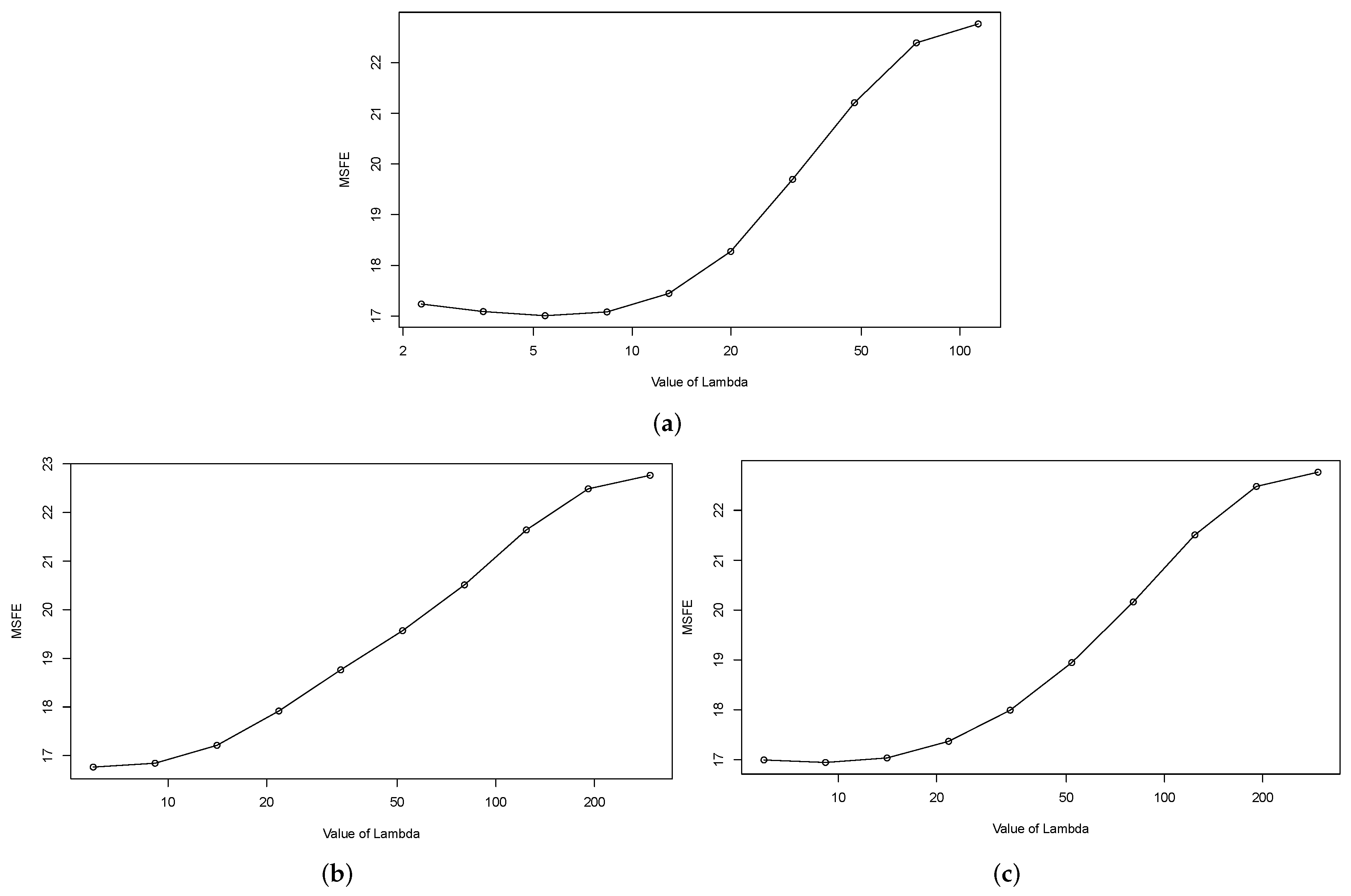
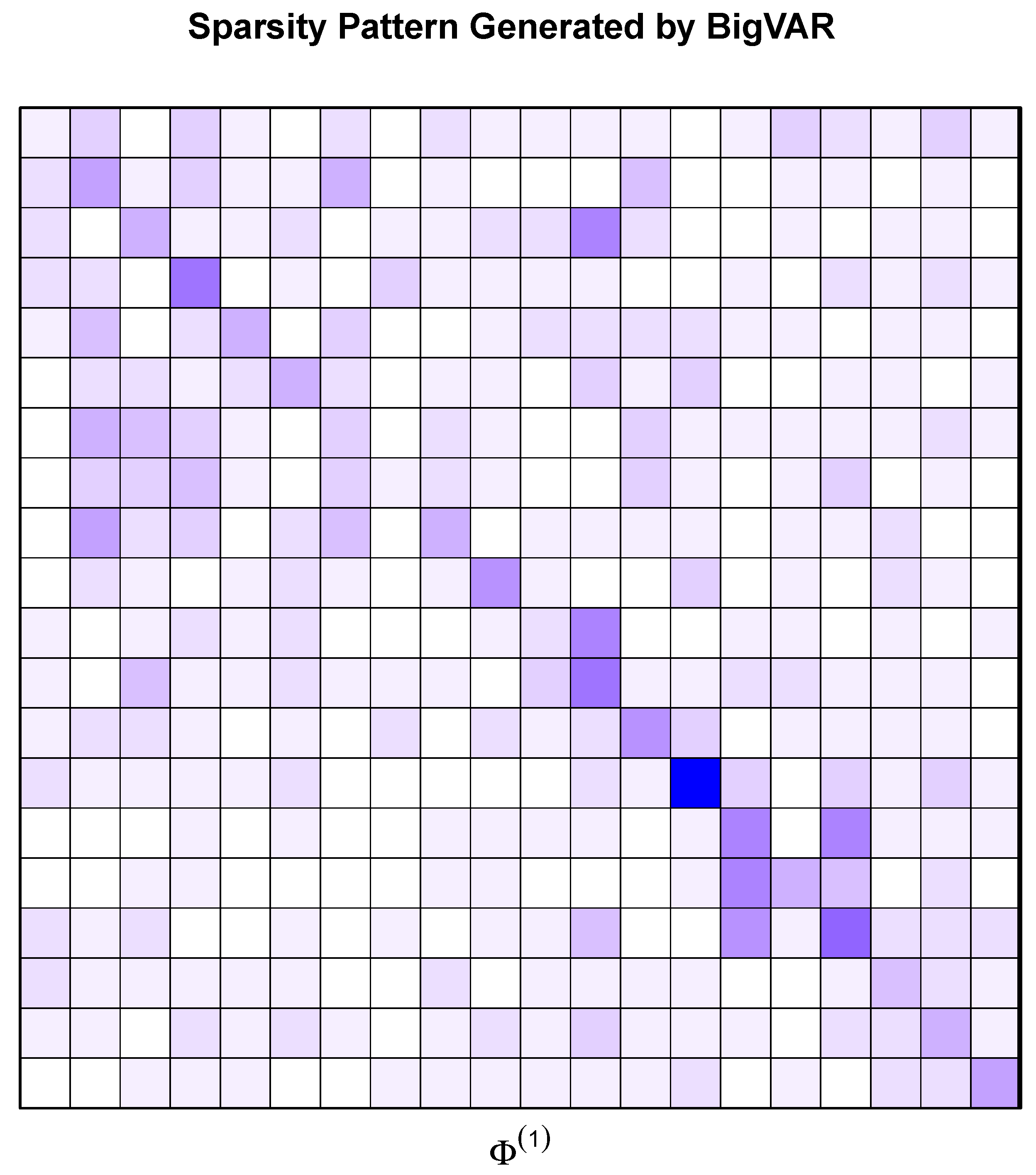
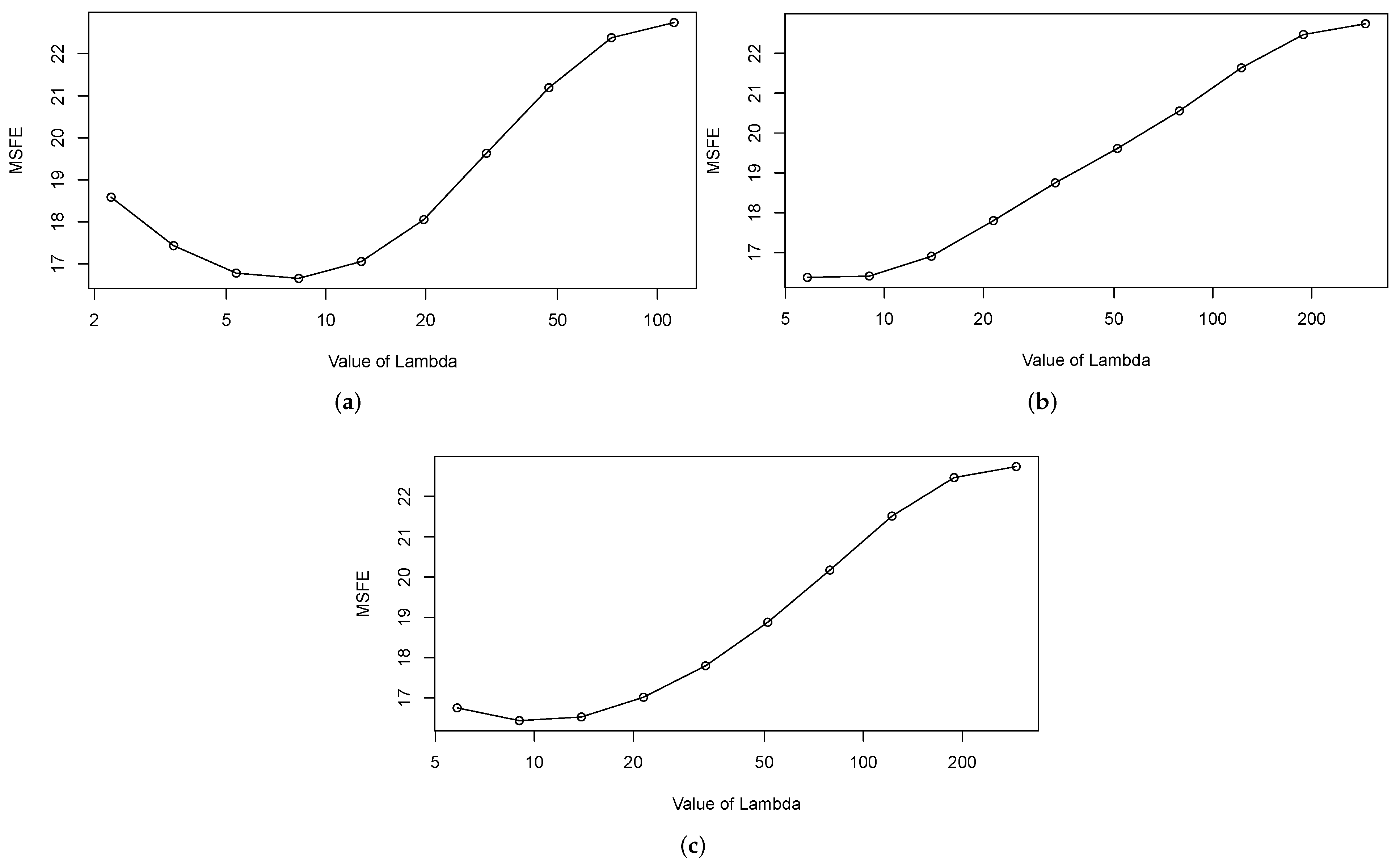
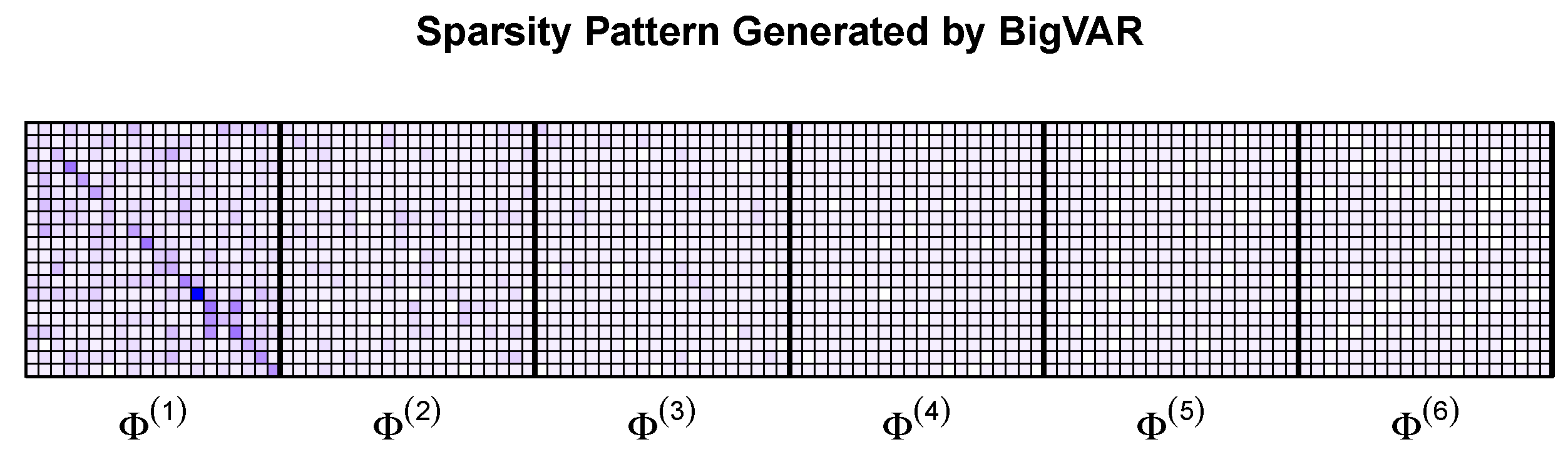
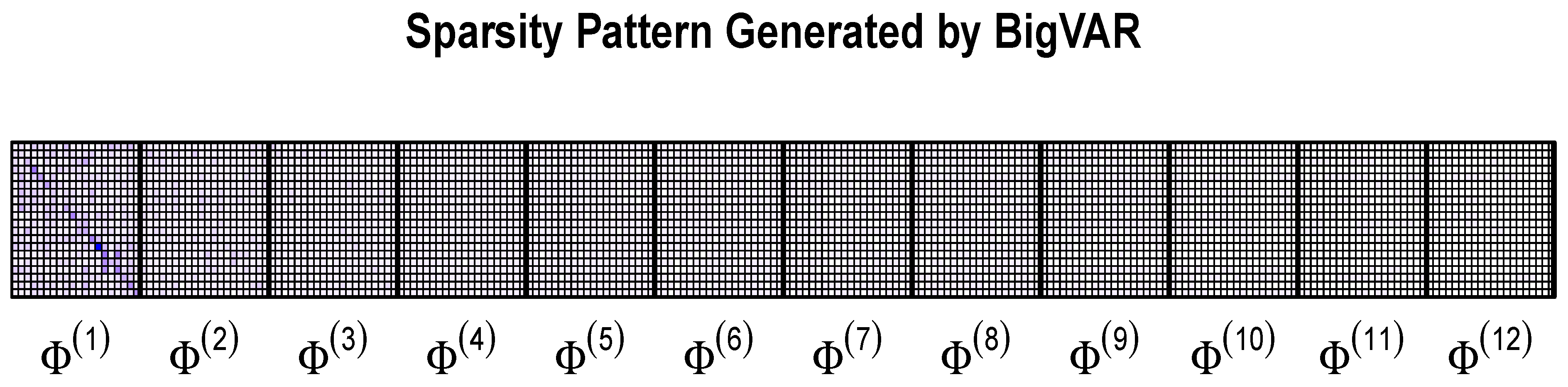
An analysis of the cross-validation (CV) behavior and the sparsity matrices of the regularization methods are also provided. Ideally, the value of $\lambda$ would increase with the forecasting horizon (h), by reflecting the U shape of the CV curve. Similarly, the sparsity should increase with the horizon.

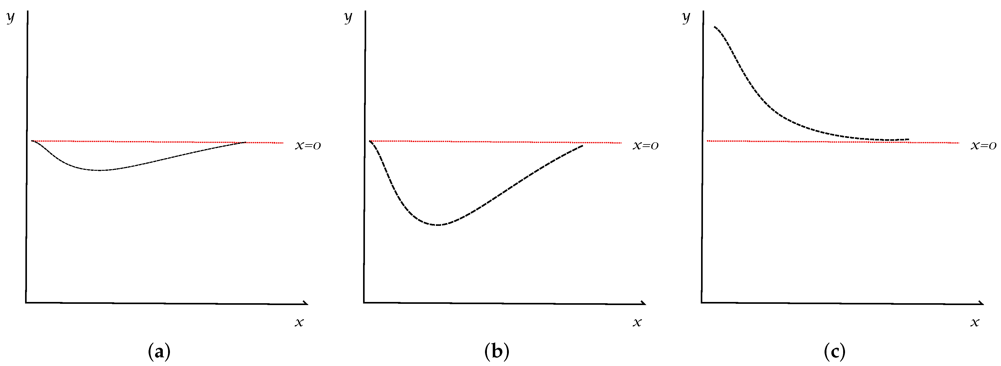
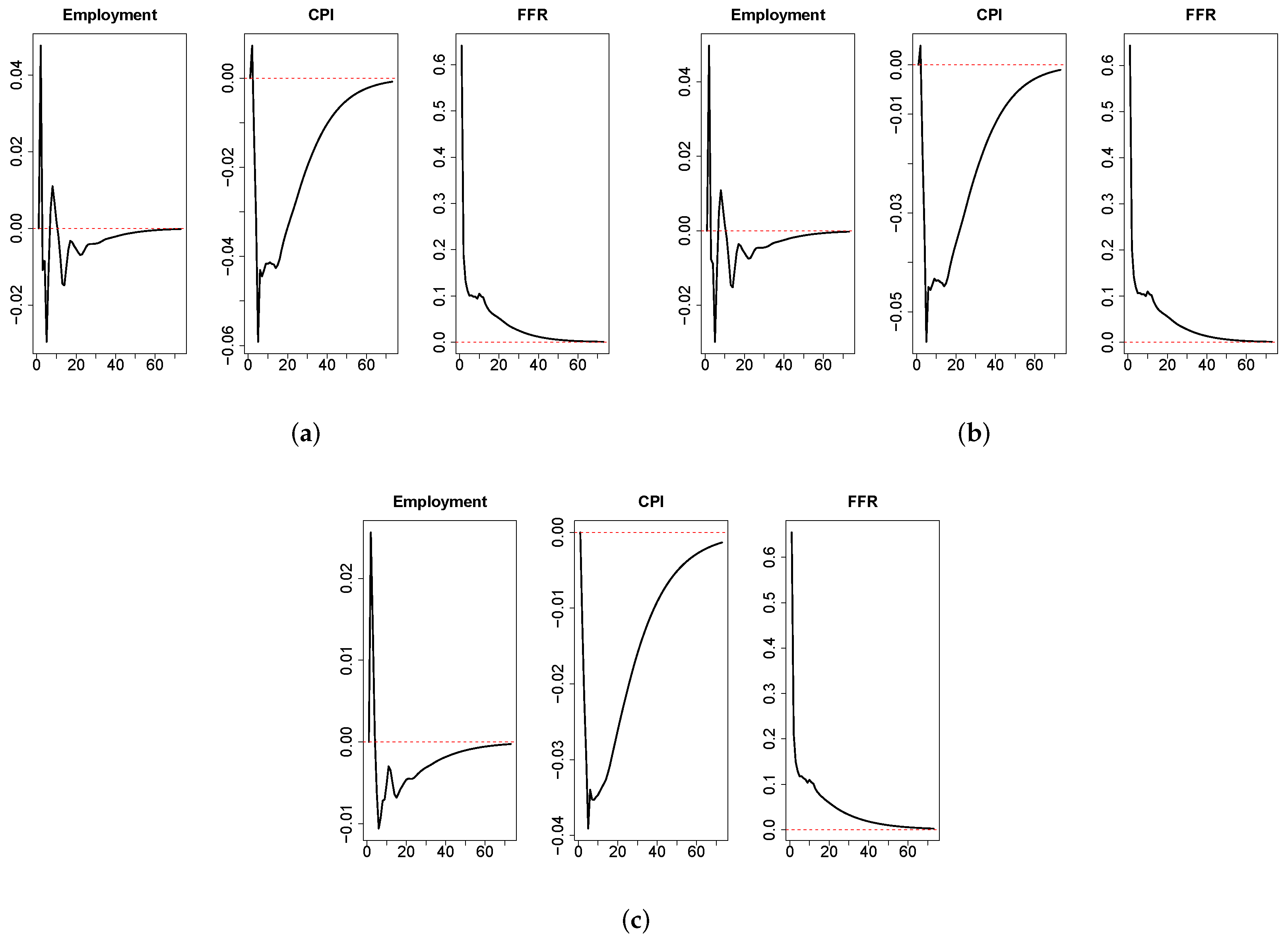
Another fundamental task of VAR models in macroeconomics, financial economics and applied time series econometrics is structural analysis. To analyze the robustness of the regularized VARs in this field, we report the Impulse Response Functions (IRF) of the models. For the sake of simplicity, we report the behavior of a variable of economic activity (employment), and a variable of inflation (consumer’s price index) after an interest rates shock of the central bank (a positive shock of one standard deviation in the federal funds rate). Due to economic theory and evidence, we expect that the IRFs behave as in Figure 1.

Therefore, if the behavior of the empirical IRFs is similar to Figure 1, there is evidence that the structural analysis methods of machine learning regularized VARs are consistent with economic theory and evidence. To ensure robustness, a hundred runs of the IRF estimates are performed via bootstrap methods.

2.2. Data and Variables

This paper uses the [34] dataset, which covers monthly macroeconomic and financial indicators from 1959 to 2003. Following [19], we are going to employ twenty variables of the dataset:

• Employment levels as a measure of economic activity.
• The consumer’s price index as a measure of inflation.
• The federal funds rate as a measure of the central bank monetary policy interest rate.
• The index of sensitive material prices.
• Monetary aggregates such as:

  (a)

  Non-borrowed reserves.

  (b)

  Total reserves.

  (c)

  The M2.

• Personal income.
• Real consumption.
• Industrial production.
• Capacity utilization.
• Unemployment rate.
• Housing starts.
• Producer price index.
• Personal consumption expenditures price deflator.
• Average hourly earnings.
• The M1.
• Standard and Poor’s stock price index.
• Yields on 10 years of the US treasury bonds.
• The effective exchange rate.

The data are log-differentiated, to ensure stationarity and ergodicity, and normalized, as usual in the regularization literature [28].

3. Results

3.1. Forecasting

3.1.1. Nowcasting

Table 1. Nowcasting MSFE of the different regularization methods against their alternatives. The smaller the quantity, the better the relative performance of the method. Source: Own elaboration.

	Componentwise	Own/Other	Elementwise	LASSO
C. Mean	0.95	0.94	0.94	0.96
AIC	0.98	0.97	0.97	1
BIC	0.89	0.89	0.89	0.91
Random walk	0.55	0.55	0.55	0.56
Bayesian VAR	0.82	0.81	0.81	0.83

shows the one-period ahead point forecast MSFE ($p=1$) of the different regularization variants in comparison with the conditional mean, the AIC and BIC selection, and a random walk. Table 1 also shows the results against the immediate alternative, the Bayesian VAR.

In any case, all regularization methods beat their alternatives except for the lag weighted LASSO which is equaled by the AIC. Additionally, all the regularization methods perform close to a 20% better than their large VAR closest alternative, the Bayesian VAR.

Table 2. A comparison of the nowcasting performance between the different regularization methods. The smaller the quantity, the better the relative performance of the method. Source: Own elaboration.

	Componentwise	Own/Other	Elementwise	LASSO	Bayesian
Componentwise	−	0.998	0.992	1.0159	1.2178
Own/Other	1.0072	−	0.999	1.0233	1.2266
Elementwise	1.0073	1.000	−	1.0234	1.2266
LASSO	1.0159	0.9772	0.9771	−	1.1986
Bayesian	0.8211	0.8153	0.8152	0.8342	−

offers a comparison between the different machine learning regularization methods and the Bayesian VAR. Each variable in a column is compared with the corresponding row.

For nowcasting, the best performing regularization method is the elementwise structure, followed by the own/other structure. The componentwise is the third best structure and, finally, the LASSO is the worst. All the regularization methods outperform the Bayesian VAR except for the lag weighted LASSO.

Figure 2 shows the cross-validation behavior of the different regularization alternatives. The y-axis is the MSFE and the x-axis the value of $\lambda$. Optimal lambdas are reached at ${\lambda }_c=5.4249$, ${\lambda }_o=5.9119$ and ${\lambda }_e=9.1307$.

The componentwise and the elementwise structures show inverted U paths. The own/other structure is closer to a linear trend. Figure 3 shows the sparsity pattern of the best regularization structure (the elementwise regularization).

As shown in Figure 3, the elementwise structure maintains an equilibrated sparsity balance. Eventually,

Table 3. A comparison of the computational time of the regularization methods in nowcasting. Source: Own elaboration.

	Time	Relative Performance (against Componentwise)
Componentwise	00:05.65	$100\%$
Own/Other	00:01.98	$35\%$
Elementwise	00:02.70	$48\%$
LASSO	00:58.23	$1030\%$
Bayesian	00:32.74	$579\%$

shows the computational time of each method.

3.1.2. Short Term

Consider a six-period ahead ($p=6$) forecasting setting as the short-term forecasting framework. The same as with the nowcasts,

Table 4. Short term forecasting $p=6$ MSFE of the different regularization methods against their alternatives. The smaller the quantity, the better the relative performance of the method. Source: Own elaboration.

	Componentwise	Own/Other	Elementwise	LASSO
C. Mean	0.95	0.96	0.97	1.35
AIC	0.90	0.92	0.93	1.29
BIC	0.93	0.95	0.95	1.33
Random walk	0.55	0.56	0.56	0.79
Bayesian VAR	0.89	0.91	0.91	1.27

offers the relative six-period ahead point forecast MSFEs of the regularization variants.

Every regularization method improves substantially against the AIC selected VAR, but gets worse against the BIC selected VAR, in comparison with nowcasts. This is mostly due to an improvement in the MSFE of the BIC and a deterioration of the model. The conditional mean MSFE remains constant, but the relative values of the three first regularization methods do not. It is important to mention here the weakening of the forecasting power of the LASSO, as the MSFE gets much higher at $p=6$, and it gets worse results that every other alternative, with the exception of the random walk. The opposite occurs with the Bayesian VAR, which improves substantially at $p=6$ in comparison with $p=1$ against any alternative or regularization method, and surpasses the LASSO. Still, the componentwise, own/other and elementwise regularization methods are better.

Table 5. A comparison of the short term $p=6$ performance between the different regularization methods. The smaller the quantity, the better the relative performance of the method. Source: Own elaboration.

	Componentwise	Own/Other	Elementwise	LASSO	Bayesian
Componentwise	−	1.0214	1.0054	1.4309	1.1224
Own/Other	0.9789	−	0.9728	1.0054	1.0988
Elementwise	1.0062	1.0279	−	1.4399	1.1295
LASSO	0.6988	0.7138	0.7177	−	0.7844
Bayesian	0.8909	0.9100	0.9149	1.2748	−

shows a comparison of the regularization methods and the Bayesian VAR.

In the short-term framework, the componentwise structure is the best regularization method. As opposed to the nowcasting framework, now the second best method is the elementwise structure, followed by the own/other structure. Another difference with the nowcasting setting is that the Bayesian VAR beats the LASSO, in concordance with the results of Table 4.

Figure 4 drops the results about the cross-validation behavior of the three first regularization methods in the short-term setting. This time, the optimal lambdas are higher and are reached at ${\lambda }_c=8.2799$, ${\lambda }_o=5.829$ and ${\lambda }_e=9.006$.

The behavior of the componentwise model improves with respect to the nowcasting setting. Now, the curve is very similar to an inverted U, and the optimal lambda increases in about 4 points as the forecasting horizon increases. The elementwise model also improves, although the optimal lambda remains stable. In the case of the own/other structure, the curve still is very similar to a linear trend.

Figure 5 shows the sparsity pattern of the best alternative, the componentwise model.

The first sparsity matrix has a substantial amount of nonzero elements, whilst the fifth matrices left are balanced.

3.1.3. Long Term

In this subsection, we are going to consider a long-term forecasting setting as a 12-period ahead forecast framework ($p=12$).

Table 6. Long term forecasting ($p=12$) MSFE of the different regularization methods against their alternatives. The smaller the quantity, the better the relative performance of the method. Source: Own elaboration.

	Componentwise	Own/Other	Elementwise	LASSO
C. Mean	0.95	0.97	1.02	1.57
AIC	0.75	0.77	0.76	1.07
BIC	0.89	0.91	0.91	1.27
Random walk	0.56	0.57	0.57	0.79
Bayesian VAR	0.91	0.93	0.93	1.29

offers the relative MSFE performance of the regularization methods against the conditional mean, AIC, BIC, random walk and Bayesian VAR.

There is a recognizable pattern which drops from Table 6. As the forecasting period increases, the AIC worsens, an so the relative performance of the regularizated VARs increases substantially. The relative performance of the regularizated VARs against the BIC also improves slightly with time, but this is mainly due to the increase of the forecasting power of the regularized VARs and not because of the worsening of the BIC. Against the random walk, the models perform much better in any case. Interestingly, Bayesian VARs relative forecasting power tends to increase with the forecasting horizon. The relative performance of them against the regularized VARs in very long horizons can be an interesting topic for further research.

Table 7. A comparison of the long term $p=12$ performance between the different regularization methods. The smaller the quantity, the better the relative performance of the method. Source: Own elaboration.

	Componentwise	Own/Other	Elementwise	LASSO	Bayesian
Componentwise	−	1.0234	1.0552	1.6576	1.1037
Own/Other	0.9771	−	1.0552	1.6197	1.0785
Elementwise	0.9261	0.9477	−	1.5350	1.0221
LASSO	0.6033	0.6174	0.6515	−	0.6658
Bayesian	0.9061	0.9273	0.9267	1.2912	−

offers a comparison of the performance of the regularization methods and the Bayesian VAR in the long-term environment.

Now, the componentwise structure continues dominating, followed by the elementwise structure. The own/other structure maintains the third position. The Bayesian VAR improves slightly, in concordance with the results of Table 6. Finally, the quality of the forecasts of the LASSO estimator declines substantially.

Figure 6 draws some results about the cross-validation analysis of the three main regularization methods in the long term. This time, the optimal lambdas are rization alternatives and are reached at ${\lambda }_c=8.1863$, ${\lambda }_o=5.7248$ and ${\lambda }_e=8.8417$.

Again, the rolling cross-validation behavior of the componentwise and elementwise structures improves. The componentwise structure has now a full inverted U form, and an optimal cross-validation behavior. The own/other curve remains flat.

Figure 7 offers the sparsity pattern of the componentwise model.

The first matrix has many nonzero elements, whilst the subsequent matrices get more sparse every period and the last matrices highly sparse.

3.2. Impulse Response Analysis

After the forecasting properties, we estimate the impulse response functions (IRF) to observe the structural analysis behavior of the machine learning regularized VARs in a monetary and financial framework. Figure 8 shows the estimated IRFs of the three regularized VARs.

A summary of the main findings dropped by Figure 6 is as follows:

• The IRFs of the three machine learning regularized VARs are consistent between them.
• The IRFs of the three machine learning regularized VARs are consistent with economic theory.
• There is very small evidence about the price puzzle in the three machine learning VARs.

The first finding is straightforward: a comparison of the three IRFs (employment, consumer’s price index and federal funds rate) between the different regularization methods (componentwise, own/other and elementwise) shows that they all follow the same path. After a sudden increase of the employment level, a shock in the standard deviation federal funds, that is to say, an unexpected contraction of the monetary policy, produces a decrease of the employment level in about the subsequent 50 periods. The three regularization methods share this behavior. Similarly, a contractionary monetary policy shock produces a decrease of the consumer’s price index for more than 60 periods in the three regularization methods. Therefore, all IRFs will behave in the same manner if we estimate a componentwise model, an own/other lag structure model or an elementwise model.

The second finding has already been pointed out. Employment and inflation decline after an unexpected increase of the federal funds rate. This is the expected behavior according to the economic theory and the macroeconomic evidence.

The third finding is not so straightforward. It starts from and it is relevant for the macroeconomics and macroeconometrics literature. The price puzzle is a situation which happens frequently when estimating monetary VARs, and refers to a positive reaction of inflation after an increase of the federal funds interest rate, when theoretically inflation is expected to decrease after a monetary policy tightening [35,36,37,38].

In this way, [39] argues that restricting the VAR to just long monetary policy lags in line with the well-known lagged effect of monetary policy eliminates the price puzzle. Our research shows that regularization methods are a valid alternative, and may be correlated with the results by [39], as these methods choose the coefficients most relevant for the VAR by their own.

Finally, it is important to mention that, counterintuitively, at the beginning, employment levels increase suddenly after a monetary contraction. This is potentially related with inventory effects [40], and might disappear when incorporating this variable to the models or at higher dimensions, what we leave open as an interesting topic for future research.

4. Discussion and Conclusions

Nowadays, vector autoregressive models are a standard methodology in the macroeconomics and finance literature to nowcast, forecast, describe data and analyze policies [9]. As the data availability increases exponentially and so the requirements for high-dimensional methods, the attention of the researchers has turned into Bayesian methods to estimate large models [19,41,42].

This research paper shows that, in this scenario, machine learning regularization methods are valid and a better alternative to Bayesian methods when estimating high-dimensional VARs. By employing the LASSO-based regularization methods proposed and computed by [28], we find that these methods perform better in nowcasting and forecasting than Bayesian VARs and all immediate comparisons. This is specially true in nowcasting and short-term forecasts as, in long-term forecasts, Bayesian methods tend to improve relatively. Nevertheless, they do not surpass machine learning regularization methods at a $p=12$ forecasting horizon.

Regarding the optimal machine learning regularization method, employing the [34] dataset, we find that in a nowcasting framework the elementwise structure is the best one, followed by the own/other structure. In short- and long-term forecasts, the componentwise structure is the best, followed by the elementwise model. With respect to the cross-validation behavior of the three models, the componentwise one appears to be the best by far, with a value of lambda which tends to increase with the forecasting horizon, as desired [19,28]. The sparsity matrices of the componentwise model show that sparsity tends to increase the higher the forecast horizon. Computationally speaking, the own/other structure is the fastest.

With respect to structural analysis, the IRFs of all three regularization methods are robust and consistent between them and with economic theory and evidence. Furthermore, we do not find any evidence of the price puzzle, and this may indicate that machine learning regularization methods are a natural alternative to structural identification assumptions such as the monetary policy long lags [39], as they may choose lags by their own. Finally, in the variable “employment level” of the economic activity, we find an effect similar to the one documented by [40], which may also be related to inventory effects.

As future research directions, first, we propose analyzing the relative performance of the Bayesian and machine learning regularized VARs in very long horizons ($h>12$), as we have detected that it tends to converge the larger the horizon (h). Second, we propose analyzing the presence of inventory and counterintuitive effects of the monetary policy in the variables related to the economic activity of the VAR in large dimensional settings ($k>20$).

References

1. Sims, C.A. Macroeconomics and reality. Econom. J. Econom. Soc. 1980, 48, 1–48. [Google Scholar] [CrossRef] [Green Version]
2. Haldrup, N.; Nielsen, F.S.; Nielsen, M.Ø. A vector autoregressive model for electricity prices subject to long memory and regime switching. Energy Econ. 2010, 32, 1044–1058. [Google Scholar] [CrossRef] [Green Version]
3. Feltenstein, A.; Iwata, S. Decentralization and macroeconomic performance in China: Regional autonomy has its costs. J. Dev. Econ. 2005, 76, 481–501. [Google Scholar] [CrossRef]
4. Cheung, W.; Fung, S.; Tsai, S.C. Global capital market interdependence and spillover effect of credit risk: Evidence from the 2007–2009 global financial crisis. Appl. Financ. Econ. 2010, 20, 85–103. [Google Scholar] [CrossRef]
5. Nick, S.; Thoenes, S. What drives natural gas prices?—A structural VAR approach. Energy Econ. 2014, 45, 517–527. [Google Scholar] [CrossRef] [Green Version]
6. Diaz, E.M.; Molero, J.C.; de Gracia, F.P. Oil price volatility and stock returns in the G7 economies. Energy Econ. 2016, 54, 417–430. [Google Scholar] [CrossRef] [Green Version]
7. Wen, F.; Min, F.; Zhang, Y.J.; Yang, C. Crude oil price shocks, monetary policy, and China’s economy. Int. J. Financ. Econ. 2019, 24, 812–827. [Google Scholar] [CrossRef]
8. Jin, X.; Zhou, S.; Yin, K.; Li, M. Relationships between copper futures markets from the perspective of jump diffusion. Mathematics 2021, 9, 2268. [Google Scholar] [CrossRef]
9. Stock, J.; Watson, M. Vector autoregressions. J. Econ. Perspect. 2001, 15, 101–115. [Google Scholar] [CrossRef] [Green Version]
10. Baumeister, C.; Kilian, L. Real-time forecasts of the real price of oil. J. Bus. Econ. Stat. 2012, 30, 326–336. [Google Scholar] [CrossRef] [Green Version]
11. Lütkepohl, H. Vector autoregressive models. In Handbook of Research Methods and Applications in Empirical Macroeconomics; Edward Elgar Publishing: Cheltenham, UK, 2013. [Google Scholar]
12. Lehna, M.; Scheller, F.; Herwartz, H. Forecasting day-ahead electricity prices: A comparison of time series and neural network models taking external regressors into account. Energy Econ. 2021, 106, 105742. [Google Scholar] [CrossRef]
13. Kim, Y.; Kim, S. Electricity Load and Internet Traffic Forecasting Using Vector Autoregressive Models. Mathematics 2021, 9, 2347. [Google Scholar] [CrossRef]
14. Bernanke, B.S.; Boivin, J.; Eliasz, P. Measuring the effects of monetary policy: A factor-augmented vector autoregressive (FAVAR) approach. Q. J. Econ. 2005, 120, 387–422. [Google Scholar]
15. Boivin, J.; Kiley, M.T.; Mishkin, F.S. How has the monetary transmission mechanism evolved over time? In Handbook of Monetary Economics; Elsevier: Amsterdam, The Netherlands, 2010; Volume 3, pp. 369–422. [Google Scholar]
16. Claeys, P.; Vašíček, B. Measuring bilateral spillover and testing contagion on sovereign bond markets in Europe. J. Bank. Financ. 2014, 46, 151–165. [Google Scholar] [CrossRef] [Green Version]
17. De Mol, C.; Giannone, D.; Reichlin, L. Forecasting using a large number of predictors: Is Bayesian shrinkage a valid alternative to principal components? J. Econom. 2008, 146, 318–328. [Google Scholar] [CrossRef] [Green Version]
18. Canova, F.; Ciccarelli, M. Estimating multicountry VAR models. Int. Econ. Rev. 2009, 50, 929–959. [Google Scholar] [CrossRef] [Green Version]
19. Bańbura, M.; Giannone, D.; Reichlin, L. Large Bayesian vector auto regressions. J. Appl. Econom. 2010, 25, 71–92. [Google Scholar] [CrossRef]
20. Ghaderpour, E. Multichannel antileakage least-squares spectral analysis for seismic data regularization beyond aliasing. Acta Geophys. 2019, 67, 1349–1363. [Google Scholar] [CrossRef]
21. Burger, M. Variational regularization in inverse problems and machine learnings. arXiv 2021, arXiv:2112.04591. [Google Scholar]
22. Lu, S.; Pereverzev, S.V. Regularization Theory for Ill-Posed Problems; Selected Topics; De Gruyter: Berlin, Germany, 2013. [Google Scholar]
23. Mohammad-Djafari, A. Regularization, Bayesian inference, and machine learning methods for inverse problems. Entropy 2021, 23, 1673. [Google Scholar] [CrossRef]
24. Emmert-Streib, F.; Dehmer, M. High-dimensional LASSO-based computational regression models: Regularization, shrinkage, and selection. Mach. Learn. Knowl. Extr. 2019, 1, 359–383. [Google Scholar] [CrossRef] [Green Version]
25. Kilian, L.; Lütkepohl, H. Structural Vector Autoregressive Analysis; Cambridge University Press: Cambridge, UK, 2017. [Google Scholar]
26. Sánchez García, J.; Cruz Rambaud, S. A GARCH approach to model short-term interest rates: Evidence from Spanish economy. Int. J. Financ. Econ. 2020, 1–12. [Google Scholar] [CrossRef]
27. Enders, W. Applied Econometric Time Series; John Wiley & Sons: Hoboken, NJ, USA, 2008. [Google Scholar]
28. Nicholson, W.; Matteson, D.; Bien, J. BigVAR: Tools for modeling sparse high-dimensional multivariate time series. arXiv 2017, arXiv:1702.07094. [Google Scholar]
29. Burkov, A. Machine Learning Engineering; True Positive Inc.: Quebec City, QC, Canada, 2020. [Google Scholar]
30. García-Pérez, J.; López-Martín, M.d.M.; García-García, C.B.; Salmerón-Gómez, R. A geometrical interpretation of collinearity: A natural way to justify ridge regression and its anomalies. Int. Stat. Rev. 2020, 88, 776–792. [Google Scholar] [CrossRef]
31. Hoerl, R.W. Ridge regression: A historical context. Technometrics 2020, 62, 420–425. [Google Scholar] [CrossRef]
32. Hastie, T. Ridge regularization: An essential concept in data science. Technometrics 2020, 62, 426–433. [Google Scholar] [CrossRef]
33. Nicholson, W.B.; Wilms, I.; Bien, J.; Matteson, D.S. High dimensional forecasting via interpretable vector autoregression. J. Mach. Learn. Res. 2020, 21, 1–52. [Google Scholar]
34. Stock, J.; Watson, M. An Empirical Comparison of Methods for Forecasting Using Many Predictors; Working Paper; Department of Economics, Harvard University: Cambridge, MA, USA, 2005. [Google Scholar]
35. Bernanke, B.S. The Federal Funds Rate and the Channels of Monetary Transmission; National Bureau of Economic Research: Cambridge, MA, USA, 1990. [Google Scholar]
36. Sims, C.A. Interpreting the macroeconomic time series facts: The effects of monetary policy. Eur. Econ. Rev. 1992, 36, 975–1000. [Google Scholar] [CrossRef]
37. Balke, N.S.; Emery, K.M. Understanding the price puzzle. In Federal Reserve Bank of Dallas Economic Review, Fourth Quarter; Federal Reserve of Dallas: Dallas, TX, USA, 1994; pp. 15–26. [Google Scholar]
38. Florio, A. Nominal anchors and the price puzzle. J. Macroecon. 2018, 58, 224–237. [Google Scholar] [CrossRef]
39. Estrella, A. The price puzzle and var identification. Macroecon. Dyn. 2015, 19, 1880–1887. [Google Scholar] [CrossRef] [Green Version]
40. Bernanke, B.S.; Gertler, M. Inside the black box: The credit channel of monetary policy transmission. J. Econ. Perspect. 1995, 9, 27–48. [Google Scholar] [CrossRef] [Green Version]
41. Carriero, A.; Clark, T.E.; Marcellino, M. Large Bayesian vector autoregressions with stochastic volatility and non-conjugate priors. J. Econom. 2019, 212, 137–154. [Google Scholar] [CrossRef]
42. McCracken, M.W.; Owyang, M.T.; Sekhposyan, T. Real-time forecasting and scenario analysis using a large mixed-frequency Bayesian VAR. Int. J. Cent. Banking Forthcom. 2021. [Google Scholar] [CrossRef] [Green Version]
Figure 1. Theoretical expected response of the variables after a one positive standard deviation central bank interest rates shock. Source: Own elaboration. (a) Employment. (b) Inflation. (c) Interest rates.
Mathematics 10 00877 g001
Figure 2. Nowcasting cross-validation behavior of the regularization methods. Source: Own elaboration. (a) Componentwise. (b) Own/other. (c) Elementwise.
Mathematics 10 00877 g002
Figure 3. Sparsity pattern of the elementwise structure. Source: Own elaboration.
Mathematics 10 00877 g003
Figure 4. Short term p = 6 forecasting cross-validation behavior of the regularization methods. Source: Own elaboration. (a) Componentwise. (b) Own/other. (c) Elementwise.
Mathematics 10 00877 g004
Figure 5. Sparsity pattern of the componentwise structure ( p = 6 ). Source: Own elaboration.
Mathematics 10 00877 g005
Figure 6. Long term p = 12 forecasting cross-validation behavior of the regularization methods. Source: Own elaboration. (a) Componentwise. (b) Own/other. (c) Elementwise.
Mathematics 10 00877 g006
Figure 7. Sparsity pattern of the componentwise structure ( p = 12 ). Source: Own elaboration.
Mathematics 10 00877 g007
Figure 8. Impulse response shocks of one standard deviation of the machine learning regularized VARs. The red dotted line is an y = 0 x-axis line. Source: Own elaboration. (a) Componentwise. (b) Own/other. (c) Elementwise.
Mathematics 10 00877 g008