An 8-Nodes 3D Hexahedral Finite Element and an 1D 2-Nodes Structural Element for Timoshenko Beams, Both Based on Hermitian Intepolation, in Linear Range

Abstract

The following article presents the elaboration and results obtained from a 3D finite element, of the 8-node hexahedron type with 6 degrees of freedom (DOF) per node (48 DOF per element) based on third degree Hermitian polynomials, and of a 2-node structural element, with 6 DOF per node (12 DOF per element), based on third degree Hermitian polynomials and the theory of Timoshenko for beams. This article has two purposes; the first one is the formulation of a finite element capable of capturing bending effects, and the second one is to verify whether it is possible to obtain the deformation of the beam’s cross section of a structural member of the beam type, based on the deformations of its axis. The results obtained showed that the 8-node hexahedron FE was able to reproduce satisfactory results by simulating some cases of beams with different contour and load conditions, obtaining errors between 1% and 4% compared to the ANSYS software, educational version. Regarding the structural element of the beam type, it reproduced results that were not as precise as the FE Hexa 8, presenting errors of between 6% and 7% with regard to the axis but with error rounding between 10% and 20%.

1. Introduction

Currently there are a large number of analytical and finite element models [1,2,3,4,5,6,7] capable of reproducing the behavior of beams with accuracy and precision. Generally, finite element models demand a considerable computational cost depending on the analysis that is proposed and the meshing established by the user.

Regarding recent developments employing Timoshenko’s beam theory, ref. [8] derived a non-local formulation using Timoshenko’s Theory and non-local elasticity, formulating the elasticity matrix using two parameters that combined the assumptions of Winkler and Pasternak. For their part, ref. [9] used the Theory of Functional Connections (TFC) to solve numerical boundary value problems. The authors solved equations that govern the response of beams using the Timoshenko–Ehrenfest Theory, which incorporates transverse shear strains.

To solve Timoshenko beams with nonlinear behavior at both geometric and material levels, the authors of [10] developed a formulation that directly applied three-dimensional nonlinear constitutive equations without zero-stress conditions. The researchers compared the results with those obtained by applying brick-type elements, managing to verify the precision and efficacy of the formulation. In another recent work, the authors of [11] incorporated interpolation functions in the Timoshenko 3D beam solution, which were obtained directly from the solution of the equilibrium differential equation of an infinitesimal deformed element, thus reducing the discretization of elements used. The interpolation functions were used in the definition of the tangential stiffness matrix in an updated Lagrangian formulation. The formulation was used to solve various three-dimensional examples with elements using different bending theories, including Timoshenko’s, achieving accurate prediction of results with minimal discretization.

To simulate the rotation phenomenon of a Timoshenko beam with different slenderness ratios, the authors of [12] implemented a 3D finite element formulation. The novelty introduced in the finite element consisted of correctly considering the moment of inertia under small rotational deformations around the equilibrium position. The authors carried out various numerical simulations that allowed them to compare the effectiveness of the formulation against commercial finite element programs. The dynamic response of Timoshenko beams has also been studied by the authors of [13], who studied perforated beams under accelerated loads in a variable thermal environment. The equations of the system have been solved numerically by means of implicit integration in time. The results obtained show correspondence with respect to the results obtained by applying conventional methods.

Another important phenomenon is the one involving lateral-torsional buckling in steel beams subjected to high temperatures. To study it, the authors of [14] have used a formulation based on Timoshenko beam-type finite elements, thus avoiding using shell-type elements that transform the problem into a much more complex and computationally expensive one. They implemented two strategies: the first one corresponded to a fiber-based beam model (FBM) and the second one corresponded to a cruciform frame model (CFM). The results obtained from the numerical simulations show an adequate reproduction of the local buckling using a reduced computational time, which represents a promising projection towards the performance-based design of this type of beam when subjected to the action of fire.

In another recent study, this time focused on the dynamic response under moving loads of fiber-reinforced Timoshenko composite beams, the authors of [15] used a Lagrangian procedure to determine the constitutive equations of motion accompanied by the use of the Ritz Method. The results obtained with the numerical simulations demonstrated the effectiveness of the formation, which, however, depends on the orientation of the reinforcing fibers and the volume fraction on the dynamic response of the models. Continuing with the Timoshenko beams, the authors of [16] studied the effect of complex loads applied at multiple nodes. The authors used the inverse finite element method (iFEM) as a basic conceptual framework and Isogeometric Analysis (IGA) as a complementary strategy to update the shape of beams in two dimensions. Numerical simulations were compared against experimental results, indicating acceptable errors for deformations.

As for finite elements applied to structural members such as beams, there are no limits to modeling, including deformations in the cross section and in the longitudinal axis, while with analytical models, only beams that have specific formulations can be modeled at a low computational cost, limiting the types of analysis of non-deformable beams that can be carried out on their cross section, and their longitudinal axis can also be modeled at a low computational cost. Commonly, for buildings design, the cross section deformation is neglected, but when the analysis requires cross section deformation, or the steel reinforcement contribution for concrete beams, it is mandatory to evaluate it by using a finite element (FE) modeling or a fiber modeling.

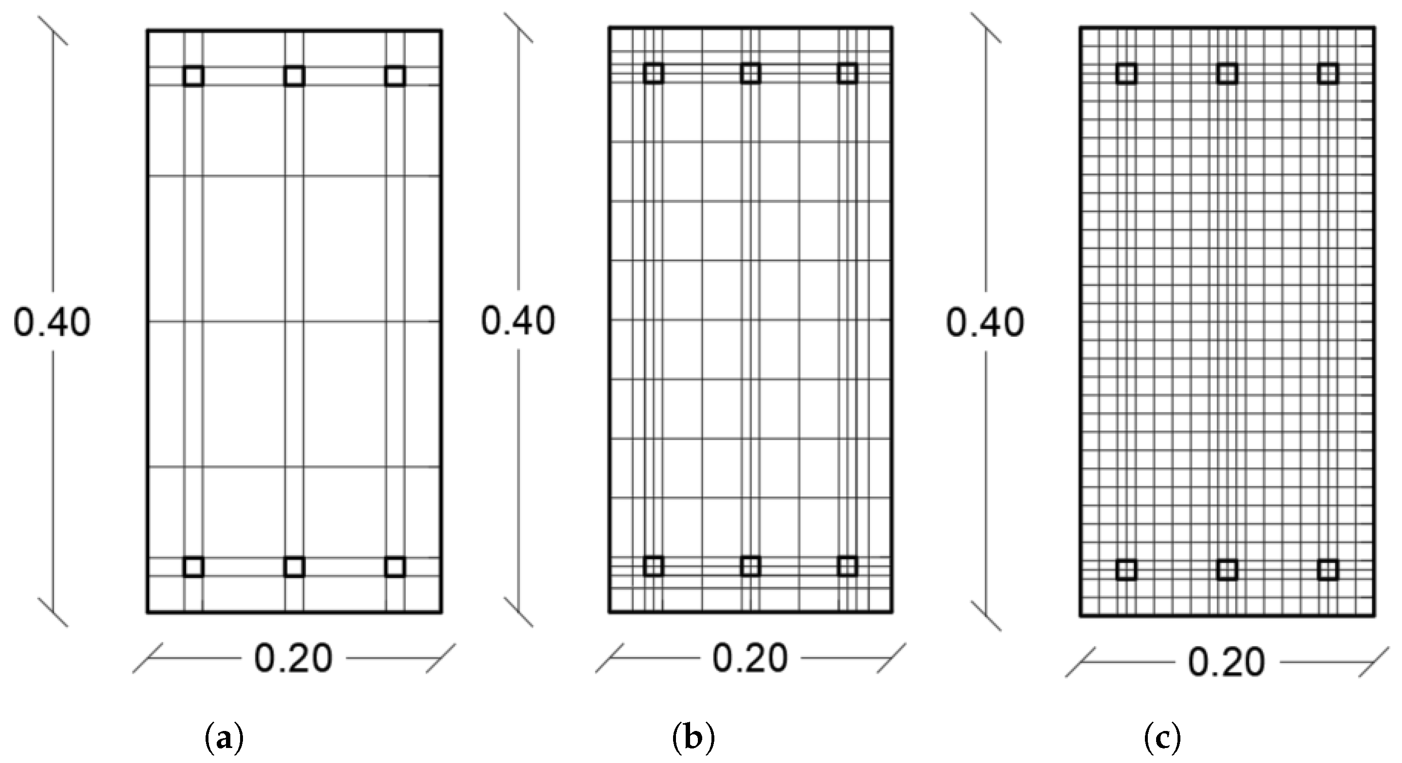
Most of 3D FE are based on tethraedrons or hexaedrons, generally with 3 DOF each node, whose shape functions are generally linear (2 nodes per edge) or quadratic (3 nodes per edge); this means, for each polinomyal degree, an extra node is needed; with this formulation, the beam’s cross section and steel reinforcement can be modeled [17,18,19,20]. For 1D FE, generally the cross section is considered through the geometrical properties within the formulation, and 6 DOF per node for full axial, shear, and bending effects. When the formulation is treated as 1D, the effects of the reinforcement in concrete beams can be represented by transforming the steel reinforcement into concrete, due to the limitations of the formulation.

When beams are being formulated, with a 3D FE or 1D FE, it is necessary a formulation capable to capture the bending and shear effects; for a 3D FE, the bending and shear effects are obtained by the three main displacements of each node, with a quadratic shape function (minimum), due to the complexity of the formulation; for a 1D FE, the formulation is quite easy, with a full 6 DOF each node (axial forces, shear forces, and bending moments). There are two main theories for beam formulation: Bernoulli’s formulation, which neglects the shear deformation (valid for small beams in heigth), and Timoshenko’s Theory, which considers the shear deformation (valid for all types of beams) [21,22,23,24,25,26].

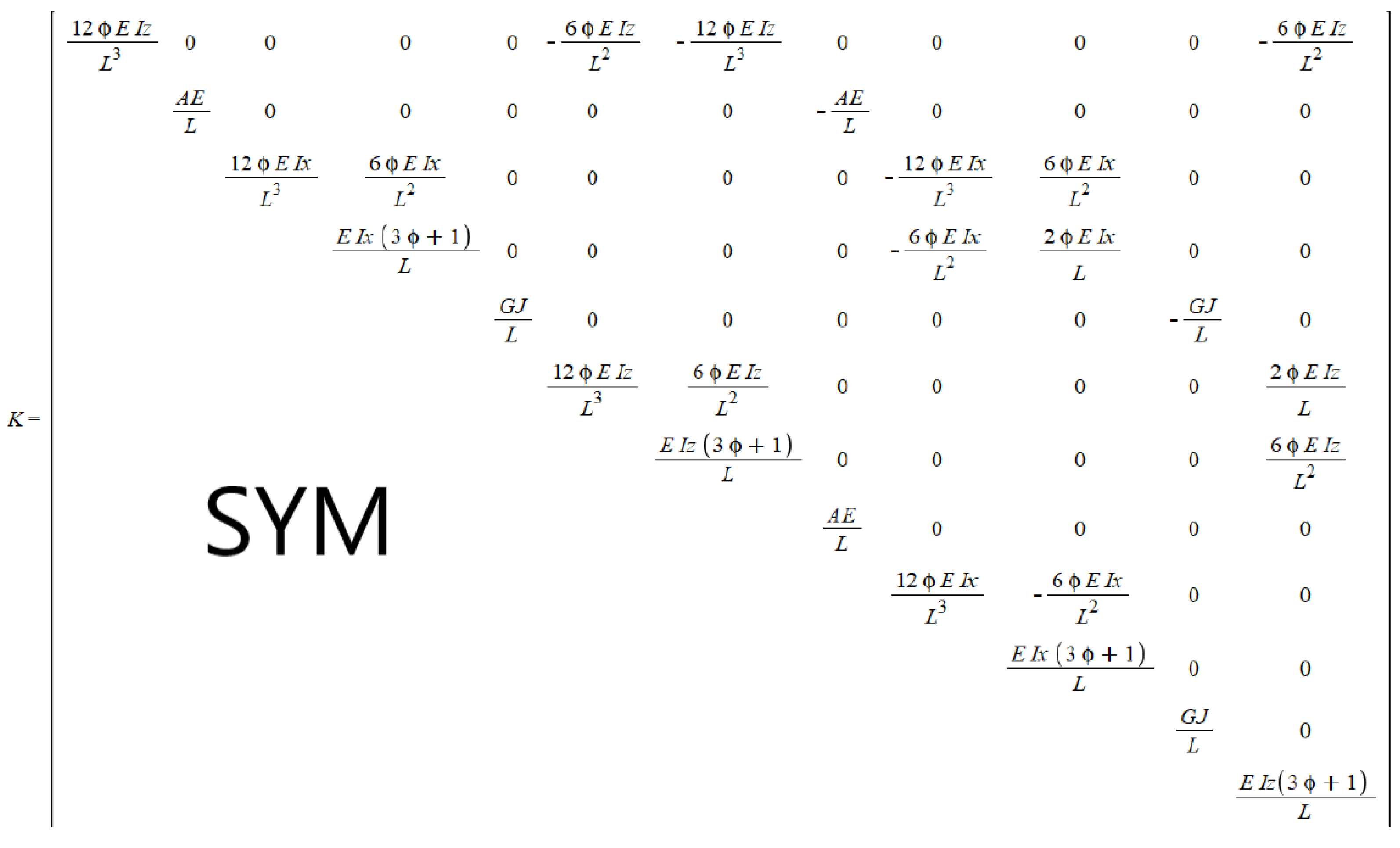
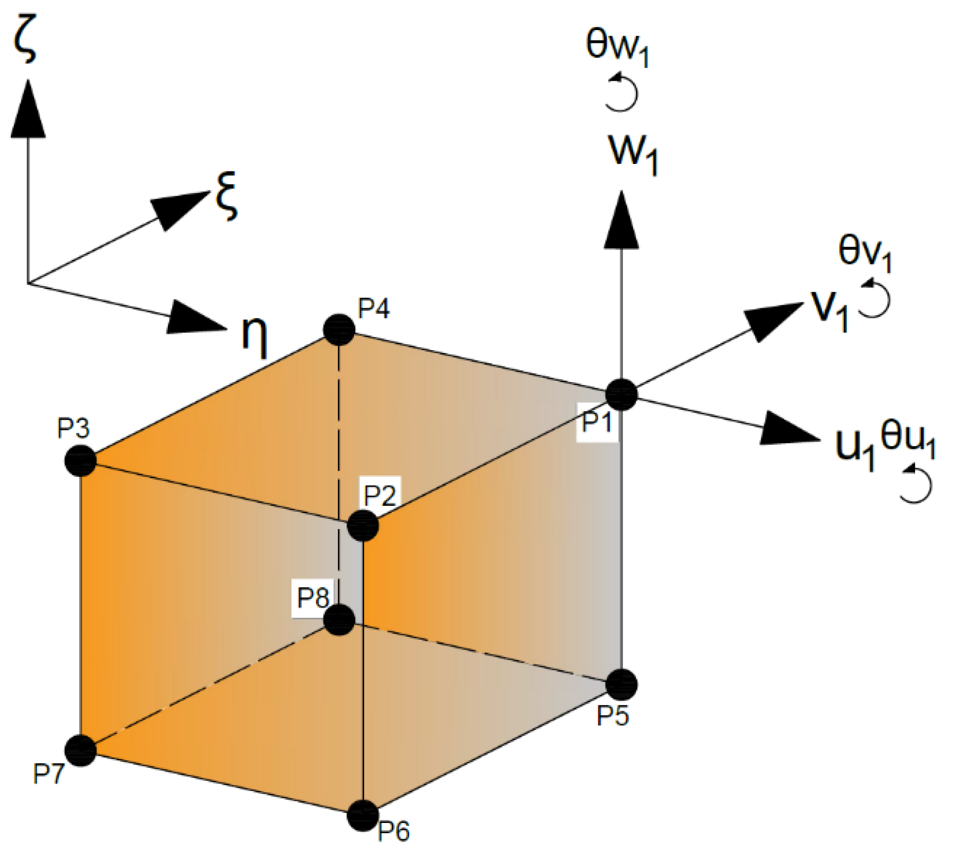
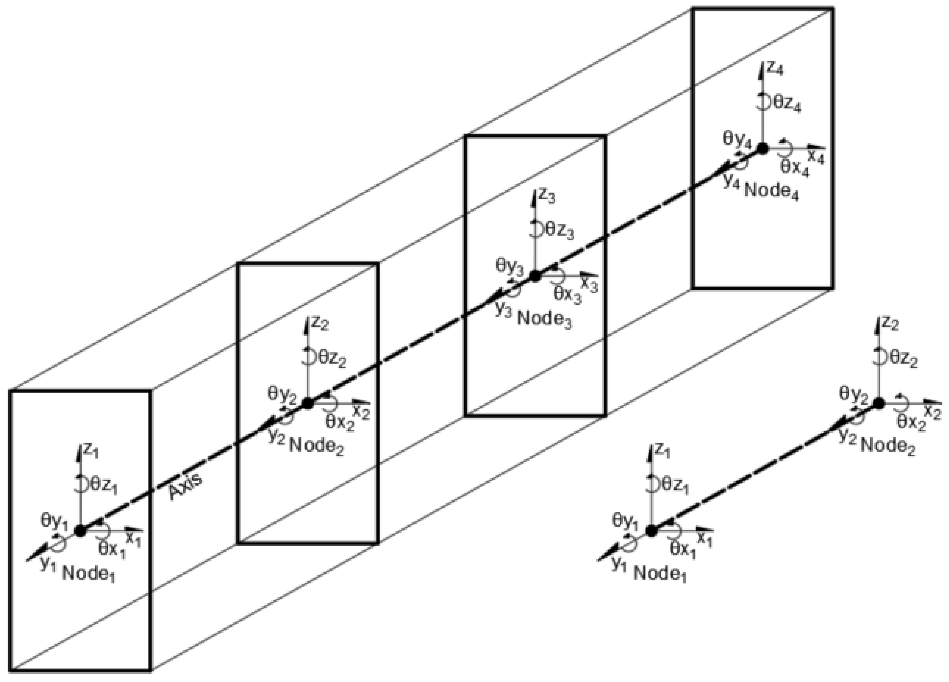
In this article, an Hexa 3D 8-node (48 DOF per element) and a 1D 2-node (12 DOF per element) will be developed, both based on their weak formulation and the Hermitian interpolation.

2. Materials and Methods

2.1. Formulation of the Hexahedral FE with 8 Nodes and 48 DOF per Element, Using Hermitian Interpolation

2.1.1. Isoparametric Formulation

This formulation has the advantage of being able to capture bending effects directly with only 8 nodes in a regular hexahedron, in the isoparametric space [7]. The hexaedron element and its DOF, in the isporametric space (which domain is $\Omega =(-1,1)$ for each edge), number of nodes and local axis, is shown in Figure 1. The hermitian polynomial for the interpolation was selected as third degree polynomial, as shown in Equation (1), which will be used to generate the shape functions for the three local axis ($\xi ,\eta ,\zeta$).

$$P(\xi )=a+b\xi +c{\xi }^2+d{\xi }^3$$

(1)

Rotation at any point of $P(\xi )$ will be $\frac{\partial }{\partial \xi }P(\xi )$, and, if the boundary conditions are taken in 2D for each edge as $\theta w_1,\theta w_2,w_1,w_2$ (Figure 2), the constants $a,b,c,d$ can be calculated as shown in Equation (2).

$$\left[\begin{array}{c}{w}_1\\ \theta w_1\\ w_2\\ {\theta }_{w_2}\end{array}\right]=\left[\begin{array}{cccc}1& -1& 1& -1\\ 0& 1& -2& 3\\ 1& 1& 1& 1\\ 0& 1& 2& 3\end{array}\right]\left[\begin{array}{c}a\\ b\\ c\\ d\end{array}\right]$$

(2)

$w_1$ and $w_2$ represent the displacement perpendicular to the edge axis for each node, while $\theta w_1$ and $\theta w_2$ represent the rotation of each node. Solving Equation (2) for constants $a,b,c,d$, with each one as a function of $\theta w_1,\theta w_2,w_1,w_2$, then grouping for $\theta w_1,\theta w_2,w_1,w_2$ and expanding the solution for each local axe, the shape functions are obtained as shown in Equation (3). It has to be noticed that the same procedure can be applied for axis $\eta$ and $\zeta$, obtaining the same equations.

$$\left[\begin{array}{c}{H}_1\left(\xi \right)\\ H_2\left(\xi \right)\\ H_3\left(\xi \right)\\ H_4\left(\xi \right)\end{array}\right]=\left[\begin{array}{c}1/4{\xi }^3-3/4\xi +1/2\\ 1/4{\xi }^3-1/4{\xi }^2-\xi /4+1/4\\ -1/4{\xi }^3+3/4\xi +1/2\\ 1/4{\xi }^3+1/4{\xi }^2-\xi /4-1/4\end{array}\right]$$

(3)

In order to construct the shape functions for each node, in the isoparametric space, a superposition of all them are proposed, as shown in Figure 3, where $H_1,H_3$ represent displacements, and $H_2,H_4$ represent rotations.

By making the superposition of the corresponding shape functions for each node, the equations for displacements and rotations are shown from Equations (4)–(11). Notice that this element is ’complete’, it means, if any equation for displacement is evaluated in any point with its coordinate, the result will be one (1), and for rotations, the result will be zero (0).

$$N{H}_1(\eta ,\xi ,\zeta )=H_3(\xi )H_3(\eta )H_3(\zeta );R{H}_1(\eta ,\xi ,\zeta )=H_4(\xi )H_4(\eta )H_4(\zeta )$$

(4)

$$N{H}_2(\eta ,\xi ,\zeta )=H_1(\xi )H_3(\eta )H_3(\zeta );R{H}_2(\eta ,\xi ,\zeta )=H_2(\xi )H_4(\eta )H_4(\zeta )$$

(5)

$$N{H}_3(\eta ,\xi ,\zeta )=H_1(\xi )H_1(\eta )H_3(\zeta );R{H}_3(\eta ,\xi ,\zeta )=H_2(\xi )H_2(\eta )H_4(\zeta )$$

(6)

$$N{H}_4(\eta ,\xi ,\zeta )=H_3(\xi )H_1(\eta )H_3(\zeta );R{H}_4(\eta ,\xi ,\zeta )=H_4(\xi )H_2(\eta )H_4(\zeta )$$

(7)

$$N{H}_5(\eta ,\xi ,\zeta )=H_3(\xi )H_3(\eta )H_1(\zeta );R{H}_5(\eta ,\xi ,\zeta )=H_4(\xi )H_4(\eta )H_2(\zeta )$$

(8)

$$N{H}_6(\eta ,\xi ,\zeta )=H_1(\xi )H_3(\eta )H_1(\zeta );R{H}_6(\eta ,\xi ,\zeta )=H_2(\xi )H_4(\eta )H_2(\zeta )$$

(9)

$$N{H}_7(\eta ,\xi ,\zeta )=H_1(\xi )H_1(\eta )H_1(\zeta );R{H}_7(\eta ,\xi ,\zeta )=H_2(\xi )H_2(\eta )H_2(\zeta )$$

(10)

$$N{H}_8(\eta ,\xi ,\zeta )=H_3(\xi )H_1(\eta )H_1(\zeta );R{H}_8(\eta ,\xi ,\zeta )=H_4(\xi )H_2(\eta )H_2(\zeta )$$

(11)

Once obtained, the shape functions in the isoparametric space, a transformation to the Cartesian space is required, through the Jacobian matrix. The shape functions can be expressed in Cartesian coordinates according to Equations (12)–(14)

$$X=\sum _{i=1}^n{\mathit{NH}}_i\left(\eta ,\xi ,\zeta \right)X_i+\sum _{i=1}^n{\mathit{RH}}_i\left(\eta ,\xi ,\zeta \right)X_i$$

(12)

$$Y=\sum _{i=1}^n{\mathit{NH}}_i\left(\eta ,\xi ,\zeta \right)Y_i+\sum _{i=1}^n{\mathit{RH}}_i\left(\eta ,\xi ,\zeta \right)Y_i$$

(13)

$$Z=\sum _{i=1}^n{\mathit{NH}}_i\left(\eta ,\xi ,\zeta \right)Z_i+\sum _{i=1}^n{\mathit{RH}}_i\left(\eta ,\xi ,\zeta \right)Z_i$$

(14)

In matrix form, the Jacobian matrix can be expressed as shown in Equation (15), and the transformation to the Cartesian coordinates is shown in Equation (16).

$$\mathbf{J}=\left[\begin{array}{ccc}\frac{\partial }{\partial \xi }x\left(\eta ,\xi ,\zeta \right)& \frac{\partial }{\partial \xi }y\left(\eta ,\xi ,\zeta \right)& \frac{\partial }{\partial \xi }z\left(\eta ,\xi ,\zeta \right)\\ \frac{\partial }{\partial \eta }x\left(\eta ,\xi ,\zeta \right)& \frac{\partial }{\partial \eta }y\left(\eta ,\xi ,\zeta \right)& \frac{\partial }{\partial \eta }z\left(\eta ,\xi ,\zeta \right)\\ \frac{\partial }{\partial \zeta }x\left(\eta ,\xi ,\zeta \right)& \frac{\partial }{\partial \zeta }y\left(\eta ,\xi ,\zeta \right)& \frac{\partial }{\partial \zeta }z\left(\eta ,\xi ,\zeta \right)\end{array}\right]$$

(15)

$$\left[\begin{array}{c}\frac{\partial }{\partial X}\\ \frac{\partial }{\partial Y}\\ \frac{\partial }{\partial Z}\end{array}\right]={\left({\mathbf{J}}^{-1}\right)}^T\left[\begin{array}{c}\frac{\partial }{\partial \eta }\\ \frac{\partial }{\partial \xi }\\ \frac{\partial }{\partial \zeta }\end{array}\right]$$

(16)

2.1.2. Elasticity Parameters

The deformation tensor, based on the six DOF per node, is shown in Equation (17) (matrix B), and the displacements matrix is shown in Equation (18). Notice that Equation (18) is showing 6 rows and 6 columns, but it is only for 1 node; hence, for the 8 nodes, the dimension of the matrix will be by 6 × 48.

$$\left[\begin{array}{c}{\epsilon }_x\\ {\epsilon }_y\\ {\epsilon }_z\\ \gamma {}_{\mathit{xy}}\\ \gamma {}_{\mathit{yz}}\\ \gamma {}_{\mathit{zx}}\end{array}\right]=\left[\begin{array}{cccccc}\frac{\partial }{\partial x}N{H}_n& 0& 0& \frac{\partial }{\partial x}R{H}_n& 0& 0\\ 0& \frac{\partial }{\partial y}N{H}_n& 0& 0& \frac{\partial }{\partial y}R{H}_n& 0\\ 0& 0& \frac{\partial }{\partial z}N{H}_n& 0& 0& \frac{\partial }{\partial z}N{H}_n\\ \frac{\partial }{\partial y}N{H}_n& \frac{\partial }{\partial x}N{H}_n& 0& \frac{\partial }{\partial y}R{H}_n& \frac{\partial }{\partial x}R{H}_n& 0\\ 0& \frac{\partial }{\partial z}N{H}_n& \frac{\partial }{\partial y}N{H}_n& 0& \frac{\partial }{\partial z}R{H}_n& \frac{\partial }{\partial y}R{H}_n\\ \frac{\partial }{\partial z}N{H}_n& 0& \frac{\partial }{\partial x}N{H}_n& \frac{\partial }{\partial z}R{H}_n& 0& \frac{\partial }{\partial x}R{H}_n\end{array}\right]\left[\begin{array}{c}{u}_n\\ v_n\\ w_n\\ \theta u_n\\ \theta v_n\\ \theta w_n\end{array}\right]$$

(17)

$$\begin{array}{c}N\end{array}=\left[\begin{array}{cccccc}N{H}_n& 0& 0& 0& 0& 0\\ 0& N{H}_n& 0& 0& 0& 0\\ 0& 0& N{H}_n& 0& 0& 0\\ 0& 0& 0& R{H}_n& 0& 0\\ 0& 0& 0& 0& R{H}_n& 0\\ 0& 0& 0& 0& 0& R{H}_n\end{array}\right]$$

(18)

The properties of the materials are shown in the Equation (19).

$$\left[\begin{array}{c}{\sigma }_x\\ {\sigma }_y\\ {\sigma }_z\\ {\tau }_{\mathit{xy}}\\ {\tau }_{\mathit{yz}}\\ {\tau }_{\mathit{xz}}\end{array}\right]=\left[\begin{array}{cccccc}2\mu +\lambda & \lambda & \lambda & 0& 0& 0\\ \lambda & 2\mu +\lambda & \lambda & 0& 0& 0\\ \lambda & \lambda & 2\mu +\lambda & 0& 0& 0\\ 0& 0& 0& \mu & 0& 0\\ 0& 0& 0& 0& \mu & 0\\ 0& 0& 0& 0& 0& \mu \end{array}\right]\left[\begin{array}{c}{ϵ}_x\\ {ϵ}_y\\ {ϵ}_z\\ {\gamma }_{\mathit{xy}}\\ {\gamma }_{\mathit{yz}}\\ {\gamma }_{\mathit{xz}}\end{array}\right]$$

(19)

2.1.3. Numerical Integration

The numerical integration used for calculations was based on Gaussian method, with 3 integration points for edge. The three main points used for the calculations were $x=[-\sqrt{\frac{5}{3}},0,\sqrt{\frac{5}{3}}]$, and $w=\frac{5}{9},\frac{8}{9},\frac{5}{9}$. The 27 integration points were obtained by the permutation of x and w.

2.1.4. Elemental Stifness and Forces Matrices

The strong formulation for the element stiffnes matrix is shown in Equation (20), while the strong formulation of the forces matrix is shown in Equation (21). The e subfix denotes the elemental matrix.

$$K_e={\int }_{\Omega }^{}{\mathbf{B}}^T\mathbf{D}\mathbf{B}\mathbf{J}\mathrm{d}\Omega$$

(20)

$$F_e={\int }_{\Omega }^{}{\mathbf{N}}^{T}q\left(x\right)\mathbf{J}\mathrm{d}\Omega$$

(21)

The strong formulation is not viable to evaluate, due to the complexity of the coordinate transformation between the isoparametric space and the Cartesian space; hence, a finite elements formulation based on the weak formulation, which implies numerical integration to the Equations (20) and (21), which become Equations (22) and (23)

$$K_e=K_e+\sum _{i=1}^n{w}_i{\mathbf{B}\left(x_i\right)}^T\mathbf{D}\mathit{B}\left({\mathit{x}}_{\mathit{i}}\right)det\left(\mathbf{J}\right)$$

(22)

$$F_e=F_e+\sum _{i=1}^n{w}_i{\mathbf{N}\left(x_i\right)}^{T}q\left(x\right)det\left(\mathbf{J}\right)$$

(23)

where:

$\mathbf{B}$ is the deformation tensor (Equation (17)). Notice that this tensor depends directly of the shape functions $(\eta ,\xi ,\zeta )$, which asume the values of the Gaussian points.

$\mathbf{N}$ is the displacements matrix (Equation (18))

$\mathbf{D}$ is the matrix which contains the materials properties (Equation (19))

$q\left(x\right)$ is the Neumann condition or boundary conditions (external forces)

n is the number of integration points

The global matrices $\mathbf{K}$ and $\mathbf{F}$ are obtained from the assembly of $K_e$ and $F_e$.

2.2. Formulation of the 1D 2-Nodes Structural Element Based on Timoshenko’s Beams Theory

In this section, a formulation of a 1D 2-nodes structural element with 6 DOF per node is based on Timoshenko’s beams theory starting from a variational formulation (this type of formulation is based on virtual work commonly), and also based on the main differential equation of displacement. Once this FE is formulated, the cross section will be deformated using geometric relationships in order to compare if, for simple beams, a deformed shape is based on the axis displacement.

2.2.1. 2D Variational Formulation (Weak Formulation)

Similar to the deduction of the beam under Bernoulli’s theory, the resolution of the Equation (24) leads to a varational formulation.

$$EI\frac{d^{4}v\left(x\right)}{d{x}^4}=q\left(x\right)$$

(24)

where I is the second moment of area of the cross section, E is the Young’s module, $v\left(x\right)$ is a displacement function, and $q\left(x\right)$ is the applied external force.

Following the general procedure, a solution is proposed by means of a test function, as shown in the Equation (25), which is integrated to reduce the order, as shown in Equation (26); this is $w\left(x\right)ϵC^4(\Omega ,\Re )$, where $\Omega =(0,L)$ is the domain of the beam; $v:\Omega \to \Re$ is the displacement at any point of the beam; and $q:\Omega \to \Re$ is the Neumann condition or boundary conditions (external forces).

$$w\left(x\right)EIz\frac{d^{4}v\left(x\right)}{d{x}^4}=w\left(x\right)q\left(x\right)$$

(25)

where:

E, is the Young’s module.

$Iz$, is the second moment of areas around the axis submited to bending moments.

$${\int }_0^{L}w\left(x\right)E\mathit{Iz}\frac{d^4}{d{x}^4}v\left(x\right)dx={\int }_0^{L}w\left(x\right)q\left(x\right)dx$$

(26)

When solving the integral by parts, and knowing that the test function $w\left(x\right)$ must have the same boundary condition (Dirichlet) as the function $v\left(x\right)$, Equations (27) and (28) are obtained.

$$w\left(x\right)E\mathit{Iz}\frac{d^3}{d^{}{x}^3}v\left(x\right)-{\int }_0^L\frac{d}{dx}w\left(x\right)E\mathit{Iz}\frac{d^3}{d^{}{x}^3}v\left(x\right)={\int }_0^{L}w\left(x\right)q\left(x\right)dx$$

(27)

$$-{\int }_0^L\frac{d}{dx}w\left(x\right)E\mathit{Iz}\frac{d^3}{d^{}{x}^3}v\left(x\right)={\int }_0^{L}w\left(x\right)q\left(x\right)dx$$

(28)

Equation (28) is solved again through integrating by parts, leading to Equation (29), where the values $w\left(L\right),w\left(0\right)$ and their derivatives evaluated at 0 and L are inputs; so, the final Equation to solve is expressed as Equation (30). $M\left(0\right)$ is the bending moment at the initial node, and $M\left(L\right)$ is the bending moment at the final node.

$${\int }_0^L\frac{d^2}{d^{}{x}^2}w\left(x\right)E\mathit{Iz}\frac{d^2}{d^{}{x}^2}v\left(x\right)={\int }_0^{L}w\left(x\right)q\left(x\right)dx+\frac{d}{dx}w\left(L\right)M\left(L\right)-\frac{d}{dx}w\left(0\right)M\left(0\right)$$

(29)

$${\int }_0^L\frac{d^2}{d^{}{x}^2}w\left(x\right)E\mathit{Iz}\frac{d^2}{d^{}{x}^2}v\left(x\right)={\int }_0^{L}w\left(x\right)q\left(x\right)dx$$

(30)

2.2.2. Finite Elements Solution

A Hermitian polynomial is proposed for the solution of Equation (3), as shown in Equation (31).

$$v\left(x\right)=d{x}^3+c{x}^2+bx+a$$

(31)

Based on Timoshenko’s beam theory, the additional shear deformation can be appended to the polynomial of Equation (31), posing a balance of shear forces, as shown in Equation (32), where the term $\mathit{Ks}GA\gamma$ represents the shear force. Timoshenko’s beam theory states that, unlike the Euler–Bernoulli’s beam theory, where the cross section does not rotate after loads are applied to it, the shear distortion v is considered as an additional rotation of the cross section. Therefore, transverse rotation and transverse displacement are considered as independent variables [22].

$$E\mathit{Iz}\frac{d^3}{d{x}^3}v\left(x\right)+\mathit{Ks}GA\gamma =0$$

(32)

where $Iz$ represents the second moment of area around the bending axis, $Ks$ is a shear correction factor depending of the cross section, G is the shear module, and A is the shear area.

In order to include this shear deformation, the value of $\gamma$ is determined from Equation (32), obtaining Equation (33), and this value is substituted in the rotation expression, as shown in Equation (34).

$$\gamma =-6\frac{E\mathit{Iz}d}{\mathit{Ks}GA}$$

(33)

$$\theta \left(x\right)=\frac{d}{dx}v\left(x\right)+6\frac{E\mathit{Iz}d}{\mathit{Ks}GA}$$

(34)

To solve Equation (34), the boundary conditions shown in Figure 2 are set, obtaining the expressions of the integration constants, as shown in Equation (35).

$$\left[\begin{array}{c}{v}_1\\ {\theta }_1\\ v_2\\ {\theta }_2\end{array}\right]=\left[\begin{array}{cccc}1& 0& 0& 0\\ 0& 1& 0& 6\frac{E\mathit{Iz}}{AG\mathit{Ks}}\\ 1& L& L^2& L^3\\ 0& 1& 2L& 3L^2+6\frac{E\mathit{Iz}}{AG\mathit{Ks}}\end{array}\right].\left[\begin{array}{c}a\\ b\\ c\\ d\end{array}\right]$$

(35)

The values of the constants $a,b,c,d$ are obtained by operating in Equation (35). Grouping the values ${\theta }_1,{\theta }_2,v_1,v_2$ and using the transformation $\varphi =\frac{1}{1+\alpha }$, $\alpha =\frac{12E{I}_z}{K_{s}GA{L}^2}$, the shape functions shown in Equations (36)–(39) are obtained.

$$N_1\left(x\right)=1-\frac{3x^2\varphi }{L^2}+\frac{2x^3\varphi }{L^3}-\frac{x\varphi (\frac{1}{\varphi }-1)}{L}$$

(36)

$$N_2\left(x\right)=\frac{x^3\varphi }{L^2}-\frac{x^2\varphi }{L}-\frac{x^2\varphi (\frac{1}{\varphi }-1)}{2L}+x\varphi +\frac{x\varphi }{2}(\frac{1}{\varphi }-1)$$

(37)

$$N_3\left(x\right)=\frac{3x^2\varphi }{L^2}-\frac{2x^3\varphi }{L^3}+\frac{x\varphi (\frac{1}{\varphi }-1)}{L}$$

(38)

$$N_4\left(x\right)=\frac{x^3\varphi }{L^2}-\frac{x^2\varphi }{L}+\frac{x^2\varphi (\frac{1}{\varphi }-1)}{2L}-\frac{x\varphi }{2}(\frac{1}{\varphi }-1)$$

(39)

Returning to Equation (30), the terms of stiffness and force are obtained, which are shown in Equations (40)–(42)

$$w\left(x\right)=\sum _{i=1}^n{w}_i·N_i\left(x\right)v\left(x\right)=\sum _{j=1}^n{v}_j·N_j\left(x\right)$$

(40)

$$K_{ij}={\int }_0^L\frac{d^2}{d{x}^2}{N}_i\left(x\right)EIz\frac{d^2}{d{x}^2}{N}_j\left(x\right)$$

(41)

$$F_i={\int }_0^L{N}_i\left(x\right)w\left(x\right)dx$$

(42)

Using Equation (41) for the indices $i=1,2,3,4$ and $j=1,2,3,4$, the stiffness matrix for bending and shear is obtained, shown in Equation (43), while the volume forces term is used Equation (42); it is shown in Equation (44). The ful 3D stiffness matrix is shown in Figure A2, and the schema for the ful 3D DOF is shown in Figure A3.

$$K_e=\left[\begin{array}{cccc}12\frac{\varphi E\mathit{Iz}}{L^3}& 6\frac{\varphi E\mathit{Iz}}{L^2}& -12\frac{\varphi E\mathit{Iz}}{L^3}& 6\frac{\varphi E\mathit{Iz}}{L^2}\\ 6\frac{\varphi E\mathit{Iz}}{L^2}& \frac{E\mathit{Iz}\left(3\varphi +1\right)}{L}& -6\frac{\varphi E\mathit{Iz}}{L^2}& \frac{E\mathit{Iz}\left(3\varphi -1\right)}{L}\\ -12\frac{\varphi E\mathit{Iz}}{L^3}& -6\frac{\varphi E\mathit{Iz}}{L^2}& 12\frac{\varphi E\mathit{Iz}}{L^3}& -6\frac{\varphi E\mathit{Iz}}{L^2}\\ 6\frac{\varphi E\mathit{Iz}}{L^2}& \frac{E\mathit{Iz}\left(3\varphi -1\right)}{L}& -6\frac{\varphi E\mathit{Iz}}{L^2}& \frac{E\mathit{Iz}\left(3\varphi +1\right)}{L}\end{array}\right]$$

(43)

$$F_e=\left[\begin{array}{c}-\frac{1}{2}w\left(x\right)L\\ -\frac{1}{12}{L}^{2}w\left(x\right)\\ -\frac{1}{2}w\left(x\right)L\\ \frac{1}{12}{L}^{2}w\left(x\right)\end{array}\right]$$

(44)

It can be seen that if shear effects are neglected due to the effects explained in Timoshenko’s beam theory, that is, $\alpha =0$, the matrix $K_e$ is equal to the one obtained by applying the Euler–Bernoulli Theory. Since what is sought is to obtain a matrix of 6 degrees of freedom per node (12 × 12 matrix), the same process can be carried out by taking into account the rotation around the z axis, resulting in a 4 × 4 $K_e$ matrix, including $Iy$ instead of $Iz$, and including axial and torsional effects.

3. Results

3.1. Validation of the Hexahedral FE with 8 Nodes

Firstly, the finite element Hexa 8 was validated for various types of beams subjected to different types of load, comparing the results with the ANSYS^® software. The cross section is 20 cm in base and 40 cm in height (Concrete, fc = 24.52 MPa, E = 23,414 MPa), to which the minimum amount of steel reinforcement has been introduced and transformed into rectangular bars. The minimum reinforcing steel yielded 6 bars of 14 mm diameter, which yielded rectangular bars 12.5 mm on a side (fy = 411.9 MPa, E = 205,940 MPa). In Figure 4, Figure 5, Figure 6 and Figure 7, the graphic at the right represents the modeling in ANSYS ^® software [27], while the graphic at the left represents the output of the finite element Hexa 8, displayed in Paraview^® software [28] and calculated using Python^® software [29]. The mesh was constructed with a Python script, and there were three different types of mesh for the cross section (Figure A1 and

Table A1. Mesh sensitivity.

Mesh	N° of Hexahedrons	N° of Nodes	Max. Vertical Displacement (m)	Error (%)
a	2240	2805	$-3.85\times {10}^{-6}$	18.113
a	3360	4080	$-4.03\times {10}^{-6}$	14.240
a	6720	7905	$-4.21\times {10}^{-6}$	10.433
a	10,800	11,730	$-4.24\times {10}^{-6}$	9.832
b	1500	2232	$-4.68\times {10}^{-6}$	0.356
b	2000	2952	$-4.71\times {10}^{-6}$	0.198
b	2500	3672	$-4.72\times {10}^{-6}$	0.461
b	3000	4392	$-4.73\times {10}^{-6}$	0.607
c	6800	8805	$-3.78\times {10}^{-6}$	19.509
c	10,200	11,760	$-3.97\times {10}^{-6}$	15.632
c	12,240	15,760	$-4.56\times {10}^{-6}$	2.983

), using the medium mesh for the validation.

The error in each simulation is shown in

Table 1. Error between ANSYS and Hexa 8 EF.

Dirichlet Condition	Neuman Condition	Displacements (mm)
		Hexa 8	ANSYS	Error (%)
One side fixed	Self weigth	$-9.87\times {10}^{-6}$	$-9.79\times {10}^{-6}$	0.79
One side fixed	Pz = −1000 N	$-1.26\times {10}^{-4}$	$-1.27\times {10}^{-4}$	0.96
One side fixed	Px = −1000 N	$-4.97\times {10}^{-7}$	$-4.98\times {10}^{-7}$	0.11
Boths sides fixed	Self weigth	$-4.21\times {10}^{-6}$	$-4.26\times {10}^{-6}$	1.21

, where the maximun error is about $3.21\%$, which means that the results for Hexa 8 FE are reliable.

3.2. Validation of the 1D 2-Nodes Structural Element for Timoshenko Beams

To determine if the deformed beam with the hypothesis is accurate in comparisson with the Hexahedral FE with 8 nodes, the evaluation of three different beams with different Dirichlet and Neuman conditions was proposed, as shown in the following paragraphs.

3.2.1. One Side Fixed Beam

This beam has the section already defined and has a length of 1 m. The results for this beam are shown in Figure 8, Figure 9 and Figure 10. The left Figure represents the EF simulation, while the right represents the Timoshenko simulation. Notice that in these results, the error has been calculated for the Timoshenko beam formulation in comparison with the Hexahedral FE with 8 nodes.

The error for each simulation, for the Timoshenko beam, is shown in

Table 2. Error for Timoshenko beams simulations.

Case	Axis	Error (%)
1	Z	2.494
2	Z	7.531
3	Y	9.348
3	Z	10.214

. Notice that errors for Timoshenko beam formulation are not negible for the torsional case (case 3), and there are several reasons for this; one reason is that for Timoshenko beam formulation, the supports were added to a single point, allowing displacements for the nodes above and below the support nodes, while for the Hexahedral FE with 8 nodes, supports were added to a surface, restricting displacements for all the support nodes. These errors, from the point of view of structural analysis, should be not allowed, due to the fact that for structural analysis the main goal is to reproduce the behavior of a real structure as well as posible; on the other hand, for structural design, even when these error values are high, for the estimation of structural cross sections, steel reinforcement, or steel profiles, these errors probably do not affect the design. For instance, a common structural parameter for acceptation or rejection of beams is the deflection or maximun vertical displacement, which is expressed in terms of the total length of the beam ($Length/480,Length/360$, among others), and if the displacements are in the order of ${10}^{-3}$ cm, with these errors, the beam still can be accepted.

Another reason could be that the deformed shape for Timoshenko beam formulation is based on linear geometric relationships, which cannot be accurate in order to estimate the deformed cross section, while with the Hexahedral FE with 8 nodes, the displacements of each node are calculated based on the FE formulation explained above. In addition, these errors were calculated as an average of the error of each point, which can be unfavorable if one point presents a huge error.

3.2.2. Double Pinned Beam

The results are presented for a beam with a length of 2 m, with pinned supports at its ends (Figure 11, Figure 12 and Figure 13). The left Figure represents the EF simulation, while the right Figure represents the Timoshenko simulation.

The error for each simulation, for the Timoshenko beam, is shown in

Table 3. Error for Timoshenko beams simulations.

Case	Axis	Error (%)
1	Z	8.129
2	Z	0.024
3	Y	0.204
3	Z	6.912

.

3.2.3. Beam with Two Pinned Supports (L = 0 m and L = 2 m) and a 1 m Cantiliever

For this beam, a length of 3 m has been considered, as shown in Figure 14, Figure 15, Figure 16, Figure 17, Figure 18 and Figure 19.

The error for each simulation, for the Timoshenko beam, is shown in

Table 4. Error for Timoshenko beams simulations.

Case	Axis	Error (%)
1	Z	10.872
2	Z	0.800
3	Z	0.567
4	Y	1.511
5	Y	17.531
6	X	19.004

.

4. Discussion

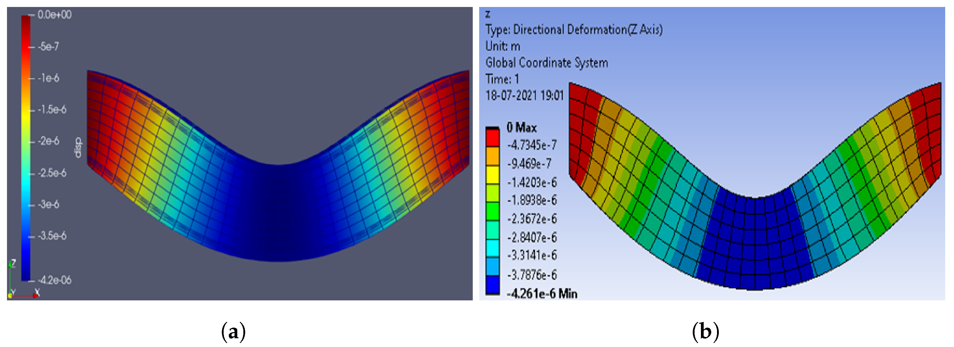
According to the results obtained, it is possible to affirm that although the results appear to be satisfactory for the structural element under Timoshenko’s theory, the error calculated in relative terms is high in some cases. In this paper, two different FE were created and evaluated, with expected results: the Hexahedral FE with 8 nodes performed better that the 1D FE Timoshenko beam formulation. In comparison, the axis displacements were relatively close, but the deformed cross section were not, essencialy with torsional effects.

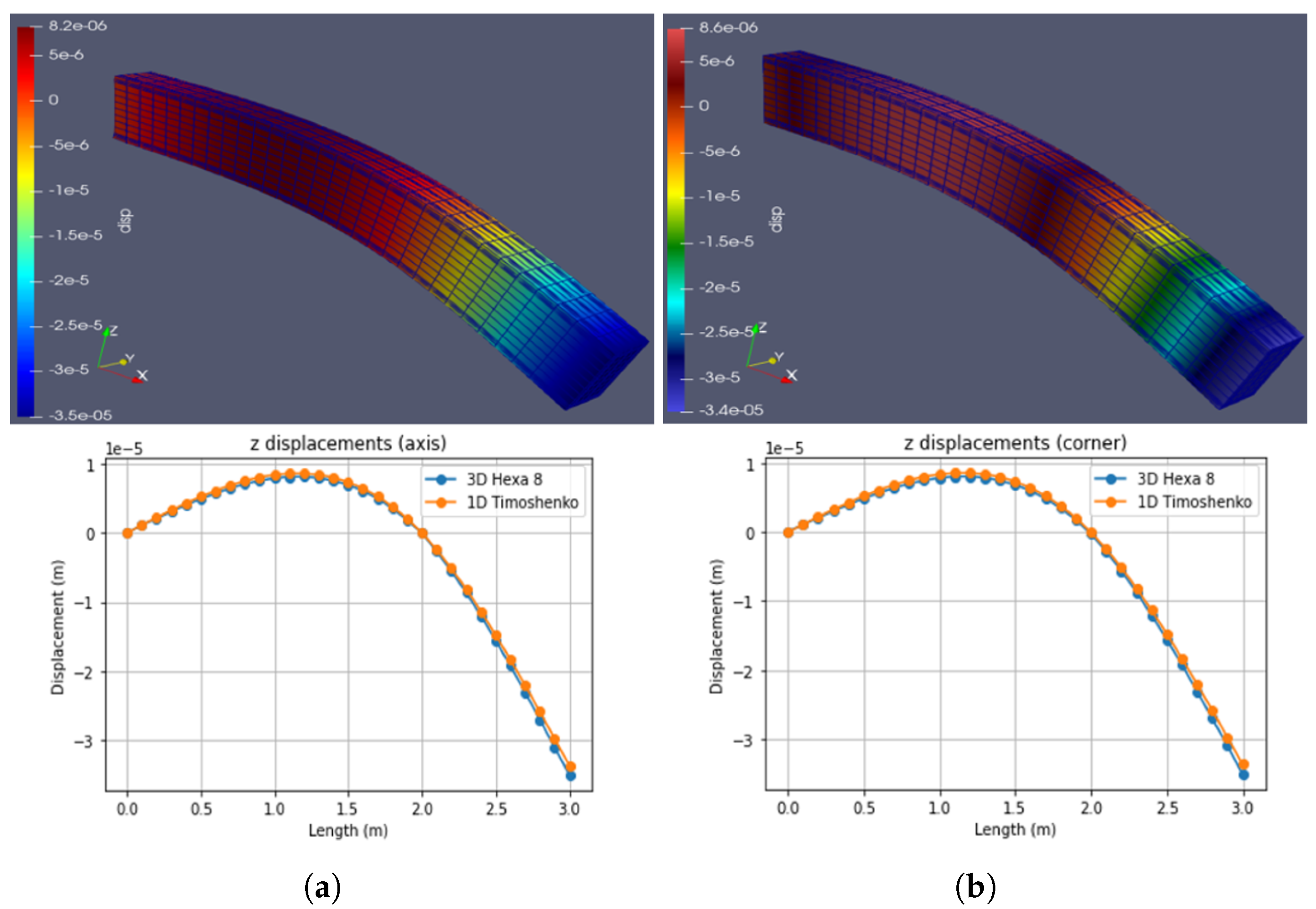
In the case of the beam embedded at one end, it is observed that in the first case (

Table A2. Ful error table for double fixed beam.

Error (%)
	Case 1	Case 2	Case 3
Length	Z	Z	Y	Z
0	0	0	0	0
0.05	72.59	21.19	69.22	86.48
0.1	57.45	14.52	43.54	38.89
0.15	47.75	10.20	33.07	29.32
0.2	40.84	7.31	26.60	24.22
0.25	35.58	5.37	22.12	20.74
0.3	31.40	4.03	18.87	18.09
0.35	27.98	3.06	16.43	15.98
0.4	25.13	2.34	14.56	14.28
0.45	22.70	1.79	13.07	12.88
0.5	20.60	1.37	11.86	11.70
0.55	18.77	1.03	10.84	10.68
0.6	17.14	0.76	9.96	9.79
0.65	15.68	0.54	9.17	8.98
0.7	14.35	0.36	8.41	8.23
0.75	13.14	0.21	7.63	7.57
0.8	12.01	0.08	6.80	7.07
0.85	10.97	0.02	5.83	6.91
0.9	9.98	0.11	4.65	7.60
0.95	9.04	0.17	3.07	9.75
1	8.13	0.23	0.20	13.75
Average	24.34	3.56	16.00	17.28

), the error is $24.34\%$ on average, while for case 2, the error remains quite low, at $3.56\%$, and for the torsional case, the values again increase to $17.00\%$ on average, which can mean important changes in the design of structures susceptible to displacement, by underestimating the maximum deflections; however, the behavior of the cross section in all cases is similar, and in addition to this, when observing the results just at the maximum length ($L=1$ m), where the maximum deflection occurs, the error is low, being the lowest of the entire table in cases 1 to 3; therefore, from the point of view of maximum deflections, the error is low.

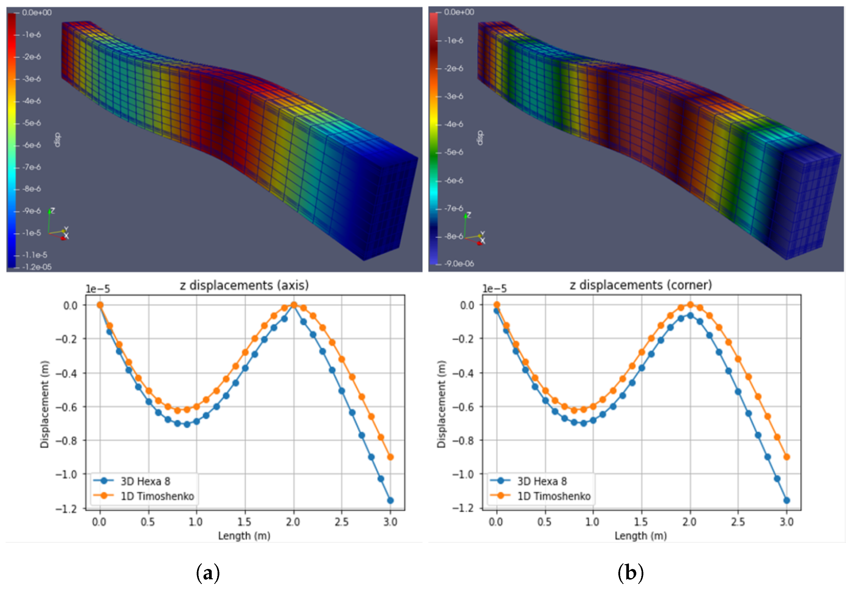
In the case of the beam articulated at both ends, it is observed that according to the

Table A3. Ful error table for two pinned supports beam.

	Error (%)
	Case 1	Case 2	Case 3
Length	Z	Z	Y	Z
0.00	0.00	0.00	0.00	0.00
0.07	22.13	20.82	60.34	68.47
0.13	11.48	12.49	35.58	31.99
0.20	7.91	10.02	25.92	24.48
0.27	5.96	8.84	20.11	19.95
0.33	4.83	8.32	16.35	16.89
0.40	4.09	8.11	13.86	14.85
0.47	3.57	8.09	12.26	13.72
0.53	3.20	8.18	11.45	13.69
0.60	2.93	8.37	11.21	14.87
0.67	2.74	8.63	12.40	19.15
0.73	2.61	8.17	10.38	13.82
0.80	2.53	7.84	9.70	11.67
0.87	2.49	7.63	9.36	10.59
0.93	2.50	7.53	9.35	10.23
1.00	2.54	7.54	9.53	10.21
1.07	2.62	7.65	9.84	10.42
1.13	2.74	7.86	10.24	10.77
1.20	2.90	8.18	10.74	11.24
1.27	3.10	8.62	11.35	11.83
1.33	3.35	9.19	12.10	12.55
1.40	3.67	9.05	13.02	13.45
1.47	4.06	8.99	14.19	14.57
1.53	4.56	9.02	15.70	16.01
1.60	5.20	9.18	17.71	17.87
1.67	6.05	9.51	20.49	20.33
1.73	7.28	10.15	24.50	23.66
1.80	9.26	11.38	30.58	28.39
1.87	12.72	13.78	40.62	36.14
1.93	22.78	21.55	66.32	73.62
2.00	0.00	0.00	0.00	0.00
Average	5.14	9.07	17.20	17.99

, the error for case 1 is low, at $5.14\%$, while the error for case 2 increases to $9.07\%$, and in the case of torsion, it continues to increase to approximately $17\%$, again, this can cause important changes in structures susceptible to displacement. Moreover, the same behavior is presented, so that the error values at the maximum deflection point ($L=1$ m) are the lowest; so, an estimate of deflections is quite close.

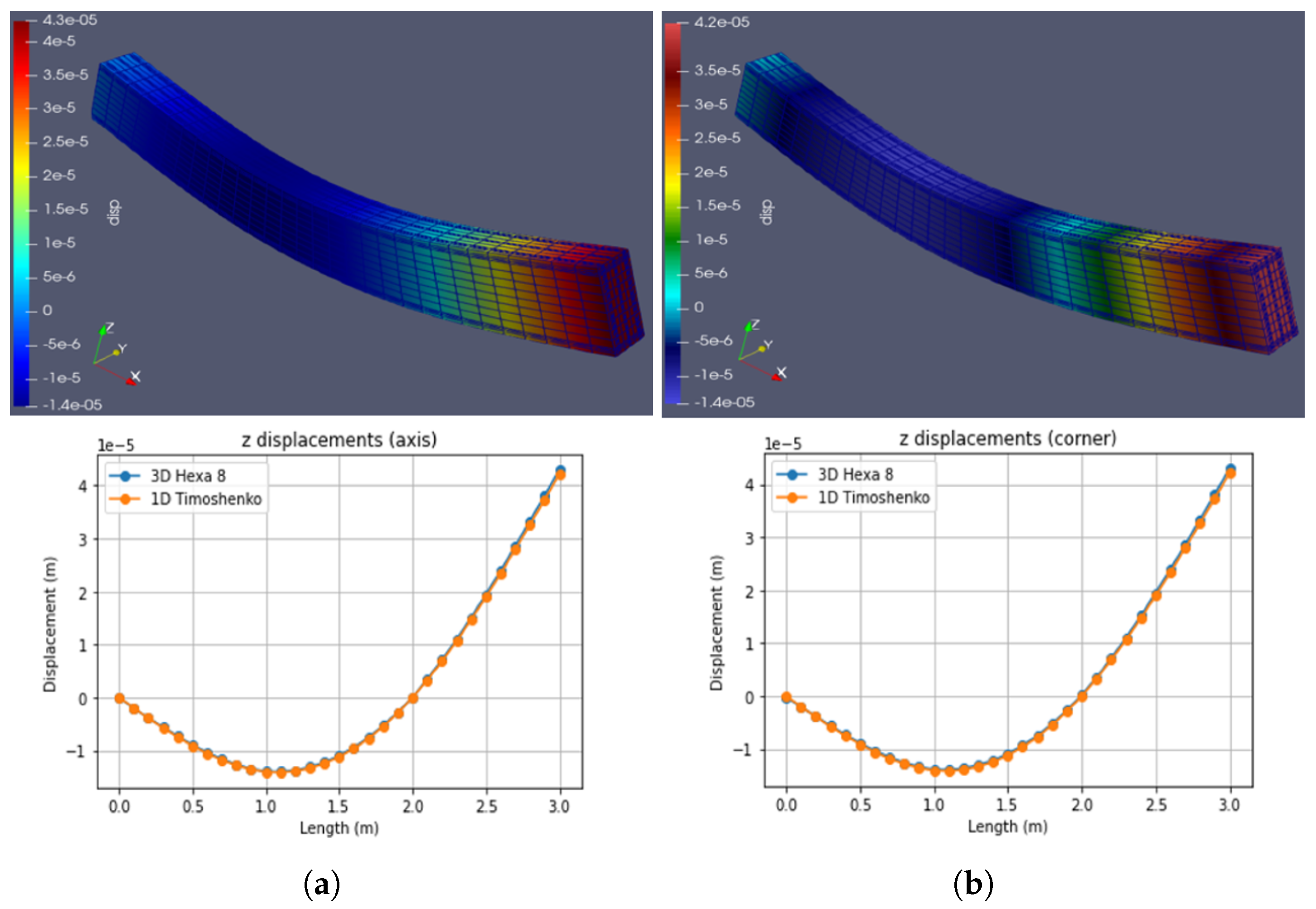
Something similar happens with the cantilever beam (

Table A4. Ful error table for two pinned supports with cantiliever beam.

	Error (%)
Length	Case 1	Case 2	Case 3	Case 4	Case 5	Case 6
0.00	0.00	0.00	0.00	0.00	0.00	0.00
0.10	24.18	0.80	3.94	100.00	78.28	100.00
0.20	15.04	5.87	1.31	100.00	62.47	100.00
0.30	12.67	6.69	2.16	100.00	51.48	100.00
0.40	11.52	6.91	2.36	100.00	43.40	100.00
0.50	11.01	6.89	2.27	100.00	37.21	100.00
0.60	10.87	6.79	2.05	100.00	32.29	100.00
0.70	11.01	6.64	1.76	100.00	28.26	100.00
0.80	11.41	6.48	1.40	100.00	24.76	100.00
0.90	12.05	6.32	1.00	100.00	21.56	100.00
1.00	12.97	6.17	0.57	100.00	17.53	100.00
1.10	14.21	6.04	0.96	100.00	20.55	100.00
1.20	15.87	5.93	1.30	100.00	22.63	100.00
1.30	18.06	5.85	1.59	100.00	24.87	100.00
1.40	21.02	5.81	1.85	100.00	27.48	100.00
1.50	25.09	5.84	2.09	100.00	30.80	100.00
1.60	30.88	5.96	2.34	100.00	35.26	100.00
1.70	39.72	6.33	2.67	100.00	41.64	100.00
1.80	53.67	7.18	3.21	100.00	51.53	100.00
1.90	78.77	11.65	5.40	100.00	68.72	100.00
2.00	–	–	–	100.00	100.00	100.00
2.10	82.87	10.77	5.83	91.28	100.00	74.49
2.20	63.64	7.34	3.90	67.48	100.00	56.80
2.30	51.67	6.25	3.31	48.30	100.00	45.73
2.40	43.36	5.57	2.94	33.85	100.00	38.64
2.50	37.42	5.11	2.69	22.91	100.00	33.58
2.60	32.93	4.76	2.50	14.46	100.00	29.69
2.70	29.41	4.48	2.34	7.84	100.00	26.57
2.80	26.58	4.26	2.22	2.61	100.00	23.87
2.90	24.21	4.09	2.13	1.51	100.00	21.18
3.00	22.16	3.88	1.99	4.76	100.00	19.00
Average	28.14	5.89	2.34	29.50	36.04	36.95

), observing high average percentages in cases 1, 4, 5, and 6, but not in cases 2 and 3; in case 1, it is observed that in the section between $L=0$ m and $L=2$ m, the lowest error occurs in the zone of maximum deflection, and in the same way in $L=3$ m, but the error is high in absolute terms. For cases 2 and 3, the behavior is the same, with a lower error value, so it can be considered acceptable. With respect to the other cases, the error has been calculated without taking into account the values of 100 because this comes from the way in which the degrees of freedom of both models are restricted, showing that for the FE model, there are some displacements that are translated between sections, while in the Timoshenko model, the displacements are restricted on the axis and no deformation is transmitted to the cross section.

5. Conclusions

As a conclusion, it can be established that the finite element 3D Hexa 8 created with Hermite polynomials accurately represents the results of the simulations when compared with a commercial software, with the disadvantage that when implemented in Python–Cython, the computation times are quite high. This finite element 3D Hexa 8 has the advantage to represent the rotations of the nodes with the translation and rotation component, which is the correct way to represent the real behavior of an element submitted to axial, bending and shear forces, in comparisson with some finite elements which the rotations are based only on the translations of each node.

The FE 3D formulation for the hexahedron was easy to formulate with third degree Hermitian polynomials due to the number of equations nedded for representing bending effects and adding the corresponding DOF for rotation, in comparison with common formulations. The proposed FE is based on hermitian polynomial interpolation, which considerably reduces the quantity of nodes in the hexahedron element and catches the bending effect more accurately by adding three additional DOF of rotation for each node. Rotations in common FE are caught by adding more nodes in the hexahedron and can include three or more nodes for each Edge, with 3 DOF for each one but only in translation, and rotations are calculated based on the translations.

It is also well known that the addition of rotations of DOF using hermitian polynomial interpolation is used for beam formulation (similar to the Timoshenko beam formulation presented in this paper) and for plates, which work with the axis of the structural element, but in this paper, the using hermitian polynomial interpolation is used directly in the FE formulation, in order to reduce the quantity of nodes and add three more DOF for rotations.

The advantage of this FE could lie in the processing time, but it depends because for a common FE formulation, there has to be a minumum of 16 nodes in order to correctly catch the bending effect (which is not very precise, because the polynomical order is barely 2), generating 48 equations per element, so the number of equations increases, but, using the Hexahedral FE with eight nodes, the number of equations is the same (48) per element but the order of the interpolation is 3 (used in this paper), not 2, so, with a common FE formulation (3 DOF per node) there will need 24 nodes, generating 72 equations per element, and it will always catch the rotations based on the translations. Based on the paragraph above, the advantages of using an FE lie in accuracy obtained by adding three additional DOF for rotations.

With respect to the Timoshenko simulations, it is observed that the results oscillate between high and low for the different beams in the different cases, so it is recommended to continue with the development until a better approximation is achieved in terms of deflections. One of the possible causes of these differences is the way in which the restrictions are carried out since by EF, these are carried out on a surface or on a line, while by the Timoshenko simulation, they are carried out at a point on the shaft, and this might make a difference.

In some cases, the Timoshenko simulations and the finite element 3D Hexa 8 matched almost perfectly, which implies that for academic purposes, it is possible to use the total section deformed shape based on the axis deformations, and by applying some trigonometric relations.

The accuracy of the finite element model must obviously be contrasted with the experimental results carried out on beams with geometry and mechanical characteristics similar to those used in this work.

References

1. Zienkiewicz, O.C.; Taylor, R.L.; Zhu, J.Z. The Finite Element Method: Its Basis and Fundamentals, 6th ed.; Butterworth-Heinemann: Oxford, UK, 2006; pp. 103–134. [Google Scholar]
2. Hughes, T.J.R. The Finite Element Method: Linear Static and Dynamic Finite Element Analysis; Dover Publications: Mineola, NY, USA, 2000; pp. 310–379. [Google Scholar]
3. Oñate, E. Structural Analysis with the Finite Element Method. Linear Statics: Volume 2: Beams, Plates and Shells; Springer Science and Business Media: Barcelona, Spain, 2013; pp. 37–43. [Google Scholar]
4. Zienkiewicz, O.C.; Taylor, R.L.; Nithiarasu, P.; Zhu, J.Z. The Finite Element Method; McGraw-Hill: London, UK, 1977; Volume 2, pp. 111–167. [Google Scholar]
5. Braess, D. Finite Elements: Theory, Fast Solvers, and Applications in Solid Mechanics; Cambridge University Press: Cambridge, UK, 2007; pp. 60–76. [Google Scholar]
6. Seshu, P. Textbook of Finite Element Analysis; Learning Private Limited: New Delhi, India, 2003; pp. 145–231. [Google Scholar]
7. Logan, D.L. A First Course in the Finite Element Method, 6th ed.; Cengage Learning: Boston, MA, USA, 2016; pp. 536–555. [Google Scholar]
8. Numanoğlu, H.M.; Ersoy, H.; Civalek, O.; Ferreira, A.J.M. Derivation of nonlocal FEM formulation for thermo-elastic Timoshenko beams on elastic matrix. Compos. Struct. 2021, 273, 114292. [Google Scholar] [CrossRef]
9. Yassopoulos, C.; Leake, C.; Reddy, J.N.; Mortari, D. Analysis of Timoshenko–Ehrenfest beam problems using the theory of functional connections. Eng. Anal. Bound. Elem. 2021, 132, 271–280. [Google Scholar] [CrossRef]
10. Choi, M.J.; Sauer, R.A.; Klinkel, S. An isogeometric finite element formulation for geometrically exact Timoshenko beams with extensible directors. Comput. Methods Appl. Mech. Eng. 2021, 385, 113993. [Google Scholar] [CrossRef]
11. Rodrigues, M.A.C.; Burgos, R.B.; Martha, L.F. A unified approach to the Timoshenko 3D beam-column element tangent stiffness matrix considering higher-order terms in the strain tensor and large rotations. Int. J. Solids Struct. 2021, 222, 11100. [Google Scholar] [CrossRef]
12. Shen, Z.; Chouvion, B.; Thouverez, F.; Beley, A. Enhanced 3D solid finite element formulation for rotor dynamics simulation. Finite Elem. Anal. Des. 2021, 195, 103584. [Google Scholar] [CrossRef]
13. Abdelrahman, A.A.; Esen, I.; Eltaher, M.A. Vibration response of Timoshenko perforated microbeams under accelerating load and thermal environment. Appl. Math. Comput. 2021, 407, 126307. [Google Scholar] [CrossRef]
14. Pallares-Muñoz, M.R.; Payá-Zaforteza, I.; Hospitaler-Pérez, A. New modeling strategies for analyzing lateral-torsional buckling in class-4 steel structural members at elevated temperatures using beam-type elements. Structures 2021, 34, 3508–3532. [Google Scholar] [CrossRef]
15. Albas, Ş.D.; Ersoy, H.; Akgöz, B.; Civalek, Ö. Dynamic analysis of a fiber-reinforced composite beam under a moving load by the ritz method. Mathematics 2021, 9, 1048. [Google Scholar] [CrossRef]
16. Chen, K.; Cao, K.; Gao, G.; Bao, H. Shape sensing of Timoshenko beam subjected to complex multi-node loads using isogeometric analysis. Measurement 2021, 184, 109958. [Google Scholar] [CrossRef]
17. Liu, G.R.; Quek, S.S. The Finite Element Method: A Practical Course, 2nd ed.; Butterworth-Heinemann, Linacre House, Jordan Hill: Oxford, UK, 2003; pp. 139–202. [Google Scholar]
18. Celigüeta-Lizarza, J.T. Metodo de los Elementos Finitos para Analisis Estructural, 3rd ed.; Unicopia: San Sebastian, Spain, 2011; pp. 15–94. [Google Scholar]
19. Long, Y.Q.; Cen, S.; Long, Z.F. Advanced Finite Element Method in Structural Engineering; Tsinghua University Press: Beijing, China, 2009; pp. 495–586. [Google Scholar]
20. Chandrupatla, T.R.; Belegundu, A.D.; Ramesh, T.; Ray, C. Introduction to Finite Elements in Engineering, 3rd ed.; Prentice Hall: Hoboken, NJ, USA, 2002; pp. 237–287. [Google Scholar]
21. Koutromanos, I. Fundamentals of Finite Element Analysis: Linear Finite Element Analysis; John Wiley and Sons: Hoboken, NJ, USA, 2018; pp. 385–424. [Google Scholar]
22. Rodrigues, M.A.C.; Burgos, R.B.; Martha, L.F. A Unified Approach to the Timoshenko Geometric Stiffness Matrix Considering Higher-Order Terms in the Strain Tensor. Lat. Am. J. Solids Struct. 2019, 16, 1–22. [Google Scholar] [CrossRef]
23. Bazoune, A.; Khulief, Y.A.; Stephen, N.G. Shape functions of three-dimensional Timoshenko beam element. J. Sound Vib. 2003, 259, 473–480. [Google Scholar] [CrossRef] [Green Version]
24. Caillerie, D.; Kotronis, P.; Cybulski, R. A Timoshenko finite element straigth with internal degrees of freedom. Int. J. Numer. Anal. Methods Geomech. 2015, 39, 1753–1773. [Google Scholar] [CrossRef] [Green Version]
25. Bui, N.N.; Ngo, M.; Nikolic, M.; Brancherie, D.; Ibrahimbegovic, A. Enriched Timoshenko beam finite element for bending and shear failure or reinforced concrete elements. Comput. Struct. 2014, 143, 9–18. [Google Scholar] [CrossRef]
26. Jafari, V.; Vahdani, S.H.; Rahimian, M. Derivation of the consistent flexibility matrix for geometrically nonlinear Timoshenko frame finite element. Finite Elem. Anal. Des. 2010, 46, 1077–1085. [Google Scholar] [CrossRef]
27. DeSalvo, G.J. ANSYS Engineering Analysis System User’s Manual; Swanson Analysis Systems, Inc.: Houston, TX, USA, 2018; 185p. [Google Scholar]
28. Henderson, A. ParaView Guide, A Parallel Visualization Application; Kitware, Inc.: Clifton Park, NY, USA, 2007. [Google Scholar]
29. Van Rossum, G.; Drake, F.L., Jr. Python Reference Manual; Centrum voor Wiskunde en Informatica: Amsterdam, The Netherlands, 1995. [Google Scholar]
Figure 1. DOF for each edge of the hexahedron.
Mathematics 10 00836 g001
Figure 2. DOF for the hexahedron.
Mathematics 10 00836 g002
Figure 3. Combination of shape functions for each node (Isoparametric).
Mathematics 10 00836 g003
Figure 4. Both sides fixed beam submitted to self weigth. (a) Paraview (Python), (b) ANSYS. (Note: e n indicates 10 n ) .
Mathematics 10 00836 g004
Figure 5. One side fixed beam, submitted to self weigth. (a) Paraview (Python), (b) ANSYS.
Mathematics 10 00836 g005
Figure 6. One side fixed beam, submitted to self weigth and a force at the non-fixed side (1000 N). (a) Paraview (Python), (b) ANSYS.
Mathematics 10 00836 g006
Figure 7. One side fixed beam, submitted to a compression force (1000 N). (a) Paraview (Python), (b) ANSYS.
Mathematics 10 00836 g007
Figure 8. Case 1: Self weigth. (a) Hexa8. (b) Timoshenko. (Note: e n indicates 10 n ).
Mathematics 10 00836 g008
Figure 9. Case 2: Horizontal (y) load at the end of the beam (1000 N). (a) Hexa8. (b) Timoshenko. (Note: e n indicates 10 n ).
Mathematics 10 00836 g009
Figure 10. Case 3: Torsional load at the end of the beam (2800 N.m). (a) Hexa8. (b) Timoshenko. (Note: e n indicates 10 n ).
Mathematics 10 00836 g010
Figure 11. Case 1: Self weigth. (a) Hexa8. (b) Timoshenko. (Note: e n indicates 10 n ).
Mathematics 10 00836 g011
Figure 12. Case 2: Pure flex. Two loads at L/3 and 2L/3 (Fz = −1000 N). (a) Hexa8. (b) Timoshenko. (Note: e n indicates 10 n ).
Mathematics 10 00836 g012
Figure 13. Case 3: Torsional load at L/3 (2800 N.m). (a) Hexa8. (b) Timoshenko. (Note: e n indicates 10 n ).
Mathematics 10 00836 g013
Figure 14. Case 1: Self weigth. (a) Hexa8. (b) Timoshenko. (Note: e n indicates 10 n ).
Mathematics 10 00836 g014
Figure 15. Case 2: At L = 3 m, Fz = −1000 N. (a) Hexa8. (b) Timoshenko. (Note: e n indicates 10 n ).
Mathematics 10 00836 g015
Figure 16. Case 3: at L = 1 m, Fz = −1000 N. At L = 3 m, Fz = −1000 N. (a) Hexa8. (b) Timoshenko. (Note: e n indicates 10 n ).
Mathematics 10 00836 g016
Figure 17. Case 4: Torsional load at L = 3 m (2800 N.m). (a) Hexa8. (b) Timoshenko. (Note: e n indicates 10 n ).
Mathematics 10 00836 g017
Figure 18. Case 5: Torsional load at L = 1 m (2800 N.m). (a) Hexa8. (b) Timoshenko. (Note: e n indicates 10 n ).
Mathematics 10 00836 g018
Figure 19. Case 6: Compression load at L = 3 m (Fx = −1000 N.m). (a) Hexa8. (b) Timoshenko. (Note: e n indicates 10 n ).
Mathematics 10 00836 g019