A Combined Experimental-Numerical Investigation of the Thermal Efficiency of the Vessel in Domestic Induction Systems

Abstract

New studies are emerging to reduce energy costs and become a more sustainable society. One of the processes where the greatest savings can be made is in cooking, due to its large-scale global use. In this vein, this study aims to analyse the influence of the vessel in the thermal efficiency at the cooking process. For that purpose, a numerical model of a cooking vessel was designed and validated with three different experimental heating tests. One of the key factors of the process is the contact between the vessel and the glass, therefore, two new approaches to model the thermal contact between the vessel and the cooktop were explored. Once the numerical models were calibrated, a full factorial analysis was performed to quantify the influence of the key parameters of the vessel in the heating process during cooking (thermal conductivity, specific heat, convection and radiation coefficients, and vessel concavity). Two of the most influential parameters in the heating process are the conductivity and the thermal contact between the vessel and the glass. Higher cooking efficiency can be achieved both with a low thermal conductivity vessel and with a high concavity, i.e., increasing the isolation between the vessel and the glass.

1. Introduction

Domestic cooking appliances have significantly evolved towards a more user-friendly and efficient use during the last decades due to the importance of cooking in our daily life [1]. One of the most important elements of the cooking process is the vessel; however, its influence on the energy efficiency has not yet been widely discussed in literature, in contrast to other domestic appliances such as gas burners and induction systems [2,3,4].

There are few studies about the vessel influence during cooking related to thermal efficiency and bottom temperature homogenisation. Cadavid et al. [5] analysed the thermal efficiency of a pot on an electric stove using numerical simulations. Villacis et al. [4] experimentally evaluated the energy efficiency of different materials for cookware used in induction systems. Hannani et al. [6] analysed the thermal efficiency of some cookings pots using a combined experimental and neural network method. Sedighi and Dardashti [7] reported that both multilayer plates and some thermal properties, such as thermal conductivity, provide a more uniform temperature profile. Ayata et al. [8] trained a neural network to find a solution to the nonregular distribution of temperature using the most efficient thickness distribution, and Karunanithy and Shafer [9] studied the efficiency of different saucepans on various cooktops and agreed that the surface finish of the pan base significantly affects the cooking efficiency.

There is no study that delves into all factors involved in the properties of cooking vessels, probably due to the difficulty of conducting these tests experimentally [4]. To address this need, we have developed high-fidelity simulations with the finite element method (FEM) and designed a full factorial analysis to study the effect of the main parameters of the vessel. The finite element (FE) model was based on a previous study [10], used to analyse the thermal distribution on the bottom of a pan depending on the meat size and position in the pan.

One of the main limitations of the FE model developed at [10] was the assumption of a constant thermal conductance between the cooking vessel and the glass. The micro-concavity of the vessel and the thermal-deformation of the vessel during the heating makes very complex to model accurately this thermal contact conductance. To address this issue, we explored two novel approaches: (I) including a layer of stratified air between the pan and the glass and (II) setting a variable thermal contact conductance in the interaction between the vessel and the glass along the radius, hereinafter referred to as Model I and Model II, respectively, see Figure 1a.

The first goal of this paper was to study how the bottom of the pan affects the cooking and in detail, the influence of the contact between the vessel base and glass. For that purpose, three FE models were calibrated independently based on experimental heating tests in three different solids: two multilayer frying pans from the Würtembergische Metallwarenfabrik (WMF) and Schulte brands and a steel plate (which was used as a flat sample). Once a high-fidelity numerical model was achieved, the key parameters of the vessel were analysed through a full factorial analysis.

This paper is organised as follows. We first describe the experimental set-up in Section 2.1: the cooktop, the three vessels under investigation and the PI control algorithm used to control the temperature of the vessel. The proposed FE models and the design of the experiments (DoE) to analyse the key parameters of the vessels under heating are explained in Section 2.2 and Section 2.3, respectively. This is followed by the results and discussion of the study and, finally, the main conclusions obtained are presented.

2. Materials & Methods

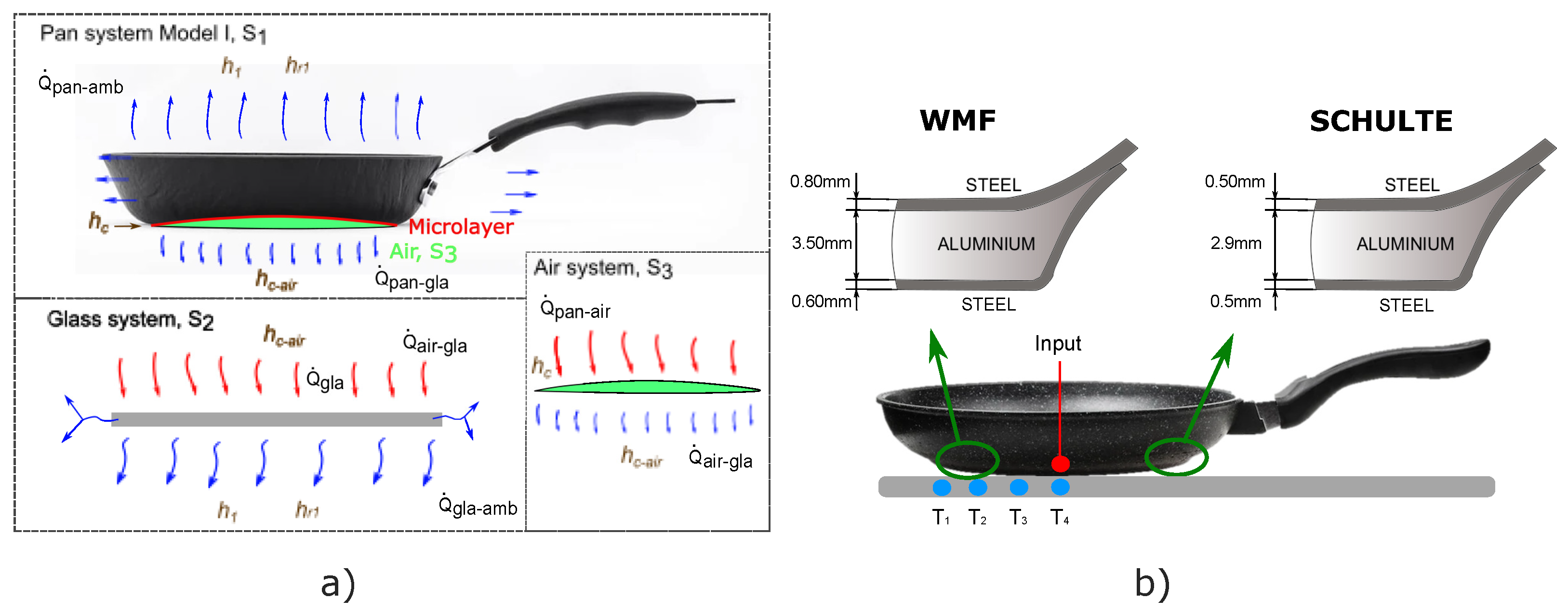
2.1. Experimental Set-Up

The experimental heating tests consisted of heating a vessel to 200 ${}^{\circ }$C for 1800 s on an induction cooktop prototype from BSH Home Appliances. The inductor used in the experiments generates a power distribution resembling a ring, which is assumed to be rotationally symmetric; see Figure 1 in Cabeza-Gil et al. [10]. The applied power turns into heat in a steel microlayer of 100 $\mathsf{\mu }$m, which is placed at the bottom of the vessel, by means of the dissipation of the eddy current density induced [11]. The power density was controlled with a PI algorithm, whose input is a thermocouple, hereinafter referred to as $T_{\mathit{sensor}}$, which was located at the centre of the cookware surface for all vessels [12]. To measure the thermal footprint in the glass, four thermocouples were placed under the glass at a radius of 7.00, 5.00, 2.00 cm and at the centre, $T_1$, $T_2$, $T_3$ and $T_4$, respectively, see Figure 1b.

Three different solids (two vessels and a steel plate) with different concavities, see Figure 2, were heated: a multilayer WMF pan with a diameter of 21 cm and a thickness of 4.9 mm (red line); a multilayer Schulte pan, model Industar, with a diameter of 20 cm and a thickness of 3.9 mm (green line); and a circular steel plate, which was specifically used in this study since its base surface is practically flat, with a diameter of 20 cm and a thickness of 6 mm (blue line). The multilayer pans consisted of three layers: steel, aluminium and steel, from bottom to top. The WMF has an aluminium volume percentage of 71.43%, while the Schulte pan has an aluminium volume percentage of 74.36%. The concavity of each vessel was measured with a Faro Prime robot with an accuracy of ±27.00 $\mathsf{\mu }$m (see Figure 2). The emissivity ($ϵ$) of each vessel under investigation was measured with a thermal emissometer, model TIR 100-2 from Inglas, along the whole spectrum.

A computer to which the experimental setup was connected calculated the supplied power required and provided it to achieve the target temperature (200 ${}^{\circ }$C) by means of the PI controller [12]. The tests for each sample were carried out three times. The software used to supply the power and to register all temperatures of the thermocouples was MATLAB R2020a.

2.2. Model Description

2.2.1. Heat Transfer Model

Two different FE models were developed to simulate the heating process of the vessels depending on how the heat transfer between the vessel and the glass was modelled. Both models were divided into two coupled systems, the vessel ($S_1$) and the glass surface ($S_2$). A new solid domain, a layer of air ($S_3$), was included in Model I to simulate the thermal contact between the vessel and the glass. In Model II, this thermal contact was modelled through a variable thermal contact conductance.

In $S_1$, ${\dot{Q}}_{pan}$ represents the heat rate generated in the ferromagnetic microlayer of the pan from the induction cooking hob. ${\dot{Q}}_{pan-amb}$ indicates the convective and radiative heat losses from the pan to the ambient environment, modelled by $h_1$ and $h_{r1}$, respectively, which are the heat transfer convective and radiation coefficients. Heat losses between the pan and the glass are different in each model because of the presence of air. In Model I, ${\dot{Q}}_{pan-air}$ depicts the heat losses to the air between the pan and the glass. In $S_2$, ${\dot{Q}}_{air-gla}$ represents the conductive heat transfer between the air and the glass and ${\dot{Q}}_{pan-gla}$ between the pan and the glass. In Model II, without the layer of air, ${\dot{Q}}_{pan-gla}$ depicts the conductive heat transfer between the pan and the glass. ${\dot{Q}}_{gla}$ is the heat absorbed by the glass, and ${\dot{Q}}_{gla-amb}$ are the convective and radiative losses from the glass to the ambient environment, which are also modelled as $h_1$ and $h_{r1}$, respectively.

The governing equations of the systems are described in Cabeza-Gil et al. [10], which come from the local heat transfer equation (Equation (1)) [13,14].

$$\left\{\begin{array}{c}\left(a\right)P={\rho }_{\mathit{SM}}{c}_{\mathit{e}-\mathit{SM}}\frac{\partial T_{\mathit{SM}}}{\partial t}-k_{SM}{\nabla }^2{T}_{SM},\Rightarrow \mathrm{SM},\\ \left(b\right)0={\rho }_{\mathit{SD}}{c}_{\mathit{e}-\mathit{SD}}\frac{\partial T_{\mathit{SD}}}{\partial t}-k_{\mathit{SD}}{\nabla }^2{T}_{\mathit{SD}},\Rightarrow \mathrm{SD}.\end{array}\right.$$

(1)

The domain of Equation (1a) is the steel microlayer (SM) of the vessel where the electromagnetic power is supplied, being P the volumetric power density generated by the induction heat source. Equation (1b) refers to the remaining part of the solid domain (SD). The terms ${\rho }_{SD}$, $c_{e-SD}$, and $k_{SD}$ are the density, the specific heat capacity and the thermal conductivity of the solid material (steel or aluminium), respectively. $T_{\mathit{SM}}$ and $T_{\mathit{SD}}$ are the corresponding temperature at some determined point in the volume domain.

Regarding the boundary conditions of the system, Equations (2) and (3) refer to the convection and radiation heat losses to the ambient environment, respectively.

$$-{\lambda }_i\frac{\partial T_i}{\partial n}=h_i(T_i-T_{amb}),$$

(2)

$$h_i=h_i^{conv}+h_i^r=h_i^{conv}+\sigma ϵ(T_i^2+T_{amb}^2)(T_i+T_{amb}),$$

(3)

where the subscript i refers to outer surface of the vessel or the glass and $\frac{\partial T_i}{\partial n}$ is the partial T-derivative normal to the reference surface. $h_i$ includes both the convective and radiative contributions, i.e., $h_i^{conv}$ and $h_i^r$ are the convective and radiative heat transfer coefficients, respectively. $\sigma$ is the Stefan–Boltzmann constant, $ϵ$ is the emissivity of the pan and $T_{amb}$ is the ambient temperature.

Thermal conduction was differently modelled for Model I and Model II. In Model I, the conduction heat losses were modelled through Equation (4) from the vessel to the air ($h_c^{va}$) and from the air to the glass ($h_c^{ag}$):

$$-{\lambda }_v\frac{\partial T_v}{\partial n}=h_c^{va}(T_v-T_a),-{\lambda }_a\frac{\partial T_a}{\partial n}=h_c^{ag}(T_a-T_g),$$

(4)

where ${\lambda }_v$ and ${\lambda }_a$ are the thermal conductivity of vessel and air. $T_v$, $T_a$ and $T_g$ are the respective temperatures at the vessel, air and glass surfaces. $h_c^{va}$ is the thermal contact conductance to be evaluated between the vessel and the air, and $h_c^{ag}$ is the thermal conductance between the air and the glass. A perfect thermal contact between the vessel and the air surface, and the air and the glass surface, was considered.

For the Model II, an iterative analysis was performed in the three samples under investigation to determine the relationship between the air gap and the thermal conductance coefficient along the radius, see Equation (5):

$$Q_c={\int }_0^R{\int }_0^{2\pi }{h}_c^{vg}\left(r\right)·\mathsf{\Delta }T\left(r\right)·r·dr·d\theta ,$$

(5)

where $Q_c$ refers to the heat loss at the contact between the pan and the glass, $h_c^{vg}\left(r\right)$ corresponds to the thermal conductance coefficient depending on the radius between the vessel and the glass, and $\mathsf{\Delta }T\left(r\right)$ is the difference in the surface temperatures in the volume domain.

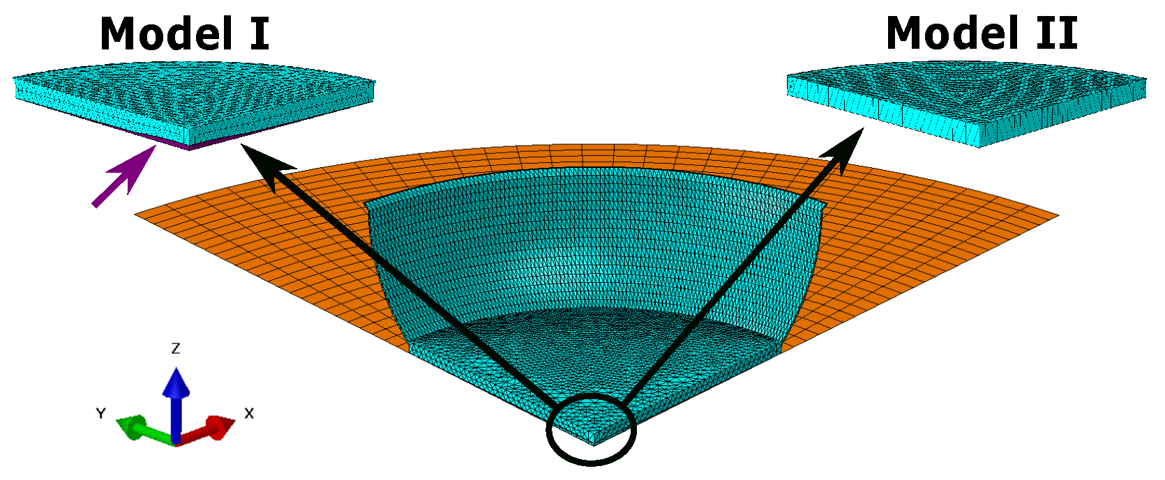
2.2.2. Finite Element Model

The FE model developed in this study is shown in Figure 3, and it is based on the study developed by Cabeza-Gil et al. [10]. The vessel geometry and the inclusion of the layer of air were different depending on the FE model analysed. Model I includes an air layer between the solid and the glass whereas Model II includes a variable thermal contact conductance. Both FE models consisted of a vitroceramic circular glass with a 200 mm radius × 4 mm thickness and the corresponding vessel previously described in Section 2.1. Due to the rotational symmetry, a quarter of the model was designed.

The commercial software Abaqus v.6.14 was used to generate the model mesh and perform the simulations. The glass was considered a shell, which was meshed with 1408 quadratic 4-node quadrilateral (DS4) and 32 3-node linear triangular (DS3) heat transfer shell elements, while the vessel (WMF, Schulte pan and steel plate) was considered a 3D solid, which was meshed with approximately 35,000 (depending on the solid) 10-node quadratic heat transfer tetrahedral elements (DC3D10); see Figure 3. For the Model I, the layer of air was approximately modelled with 200 DC3D10 elements.

The power density distribution generated by the induction system was numerically computed in an electromagnetic FE model [15,16]. The power-density field from the FE model was mapped using an in-house subroutine, which was written in MATLAB 2020a, onto the FE mesh to perform the thermal analysis. The power supplied was calculated using PI control, which is a temperature-level control, and it was added through the URDFIL and DFLUX subroutines. This control reproduces the control implemented in the experimental heating tests by determining the power supplied from the previous time increment ($\mathsf{\Delta }t=1$ s) of the temperature sensor. The target temperature in the control was 200 ${}^{\circ }$C, and the maximum power applied was limited to 2200 W, as in the experimental tests.

The whole model was at ambient temperature ($T_{amb}=23{}^{\circ }$C) as initial condition. The boundaries conditions applied to the model are described in Section 2.2.1. Briefly, convection and radiation heat losses were imposed to all external surfaces of the model. For Model I, the heat conduction between the vessel and the air, and the air and the glass, was considered through a thermal contact conductance. Whereas for Model II, the heat conduction between the vessel and the glass surfaces was considered through a variable thermal contact conductance depending on the position ($h_c^{vg}\left(r\right)$. Convective and conductance parameters used in the computational models were obtained individually for each vessel after an optimisation process by fitting the experimental tests with the numerical tests. In each vessel, the same convective parameter was applied for all external surfaces. The coefficients of the glass were the same for all simulations. The thermal air properties [14] used in the study are shown in

Table 1. Properties of air (Model I) modelled based on temperature as a continuum between the vessel and the pan [12].

Temperature (K)	Density (kg/m${}^3$)	Conductivity (W/mK)	Specific Heat (kJ/kgK)	Expansion Coefficient (-)
300	1.16	0.026	1.007	0.0037
350	0.99	0.030	1.009
400	0.87	0.034	1.014
450	0.77	0.037	1.021
500	0.69	0.041	1.030
550	0.63	0.044	1.040
600	0.58	0.047	1.051

.

2.2.3. Finite Element Method Discretization

The weak form of Equation (1a) can be written as:

$${\int }_{\mathsf{\Omega }}P\delta Td\mathsf{\Omega }={\int }_{\mathsf{\Omega }}\rho c_e\frac{\partial T}{\partial t}\delta Td\mathsf{\Omega }-{\int }_{\mathsf{\Omega }}k{\nabla }^{2}T\delta Td\mathsf{\Omega }$$

(6)

being $\mathsf{\Omega }$ the solid domain and $\delta T$ the virtual temperature. The application of classical differentiation rules to the last term of Equation (6) leads to the following statement:

$${\int }_{\mathsf{\Omega }}P\delta Td\mathsf{\Omega }={\int }_{\mathsf{\Omega }}\rho c_e\frac{\partial T}{\partial t}\delta Td\mathsf{\Omega }+{\int }_{\mathsf{\Omega }}\nabla \delta Tk\nabla Td\mathsf{\Omega }-{\int }_{\partial \mathsf{\Omega }}k\nabla T\delta Td(\partial \mathsf{\Omega })$$

(7)

The FEM discretization procedure starts from the following approximation of the temperature function:

$$T(x,y,z)=N_{\alpha }{T}_{\alpha }, \mathrm{being} \alpha =1,\dots ,n$$

(8)

where $T(x,y,z)$, the temperature in the Cartesian coordinates, is represented by $N_{\alpha }$, the shape functions, and $T_{\alpha }$, the nodal temperatures. n is the total number of degrees of freedom of the model. Following the usual approximation of FEM, the virtual temperature ($\delta T$) is identified as the shape functions, $\delta T=N_{\beta }$. The matrix form of Equation (7) is represented as follows:

$$Q_{\alpha }^{\left(e\right)}={\int }_{{\mathsf{\Omega }}^{\left(e\right)}}P{N}_{\beta }d\mathsf{\Omega }+{\int }_{\partial {\mathsf{\Omega }}^{\left(e\right)}}k\nabla T{N}_{\beta }d(\partial \mathsf{\Omega })$$

(9)

$$K_{\alpha \beta }^{\left(e\right)}={\int }_{{\mathsf{\Omega }}^{\left(e\right)}}(k_x{N}_{\alpha ,x}{N}_{\beta ,x}+k_y{N}_{\alpha ,y}{N}_{\beta ,y}+k_z{N}_{\alpha ,z}{N}_{\beta ,z})d\mathsf{\Omega }$$

(10)

$$M_{\alpha \beta }^{\left(e\right)}={\int }_{{\mathsf{\Omega }}^{\left(e\right)}}\rho c_e{N}_{\alpha }{N}_{\beta }d\mathsf{\Omega }$$

(11)

The assemblage and condensation procedures for the system matrices and vectors lead to the well-known final system of algebraic equations, which has been solved implicitly through the trapezoidal rule for time integration in Abaqus. The initial and boundary conditions needed to solve the equations system are described in Section 2.2.1.

$$M_{\alpha \beta }\frac{\partial T_{\beta }}{\partial t}+K_{\alpha \beta }{T}_{\beta }=Q_{\alpha }$$

(12)

2.3. Design of the Experiment

The influence of the key parameters of the model, the conductivity (k), specific heat ($c_e$), emissivity ($ϵ$), and concavity ($Con$) of the vessel, and the convective coefficients of the vessel ($h_v^{conv}$) and the glass ($h_g^{conv}$) in the cooking process were analysed following the DoE methodology by a full factorial analysis [17]. The simulations consisted in heating the vessel during 1800 s as in the experimental tests. A screening analysis was performed to observe the influence of each variable and decide the levels of the DoE. Based on this analysis, an intermediate value was selected for the conductivity, specific heat and concavity, whereas the remaining terms (emissivity and convective coefficients of the vessel and the glass) had two levels, resulting in 243 simulations (i.e., $3^3\times 3^2=243$ simulations), see

Table 2. Values of the analysed parameters for each level. Conductivity, specific heat and concavity have three levels, whereas both convective parameters and emissivity have only two. The steel density was considered constant with a value of 7900 kg/m${}^3$.

Process Parameters	Low Level	Intermediate Level	Maximum Level
k (W/mK)	49	142	235
$c_e$ (J/kgK)	300	420	540
$Con$	Scenario #A	Scenario #B	Scenario #C
$h_v^{conv}$ (W/m${}^2$K)	3	-	9
$h_g^{conv}$ (W/m${}^2$K)	3	-	9
$ϵ$	0.3	-	0.9

.

The maximum and minimum levels of the conductivity and the specific heat were chosen based on the properties of aluminium and steel [18]. The parameters affecting three heat losses ($ϵ$, $h_v$, $h_g$) were chosen according to values reported in the literature [10,11].

To analyse the influence of concavity, three different scenarios, see Figure 4, were considered. The red line was considered the reference case (from the WMF pan), hereinafter referred to as scenario #B. Two more scenarios where the concavity was increased by 1.5 times and decreased by 0.5 times were introduced (scenario #A and scenario #C, respectively).

The effect of the key parameters in the heating process were analysed measuring different factors of the cooking process: time to reach steady state ($t_{st}$), supplied energy during the cooking ($E_{in}$), maximum temperature of the sensor ($T_s$) and temperature homogenisation at the bottom along the radius after 1 min from the start ($H_r$):

$$H_r=1-\frac{1}{S_p}{\int }_0^{2\pi }{\int }_0^{r_{ext}}\frac{\mid \overline{T}-T(r,\theta )\mid }{\overline{T}}·r·dr·d\theta ,$$

(13)

where $H_r$ refers to the temperature homogenisation along the radius in the second 60 of the cooking, $S_p$ is the cookware surface of the pan, r is the radius of the pan, $\overline{T}$ is the mean temperature of the nodes selected in the cookware surface and $T(r,\theta )$ is the temperature in each node.

3. Results & Discussion

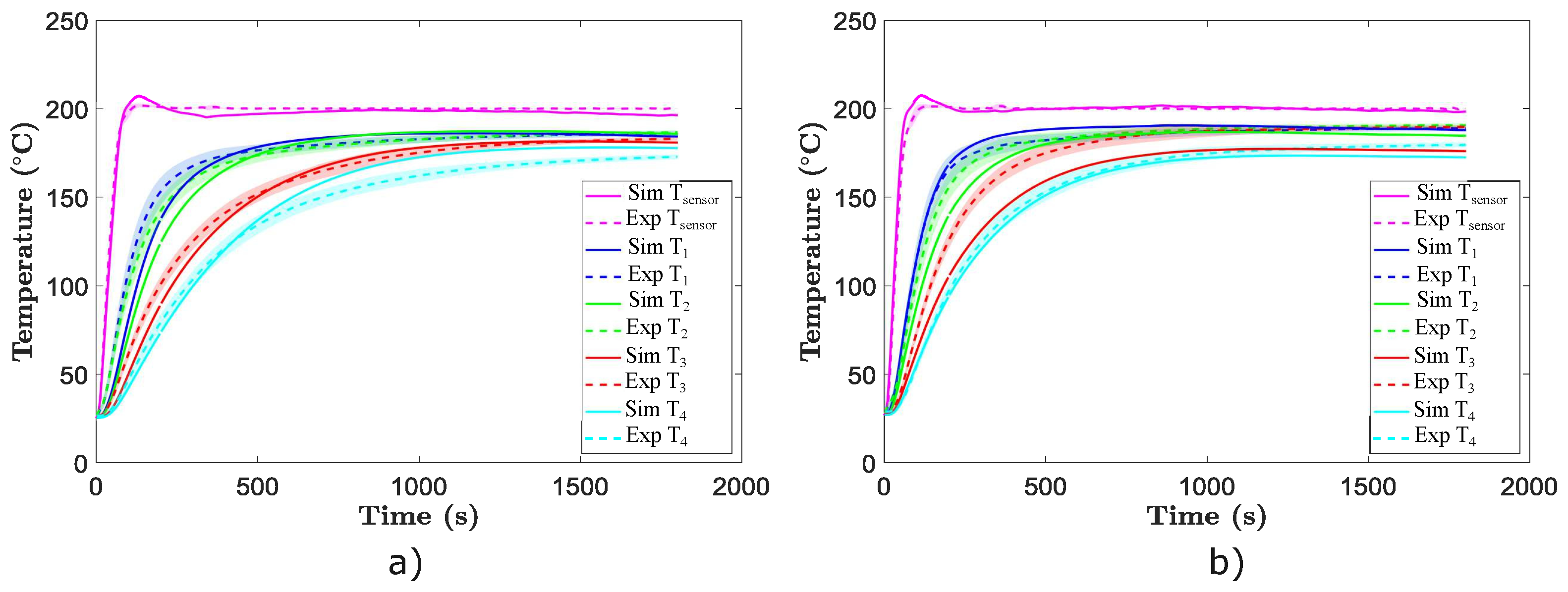
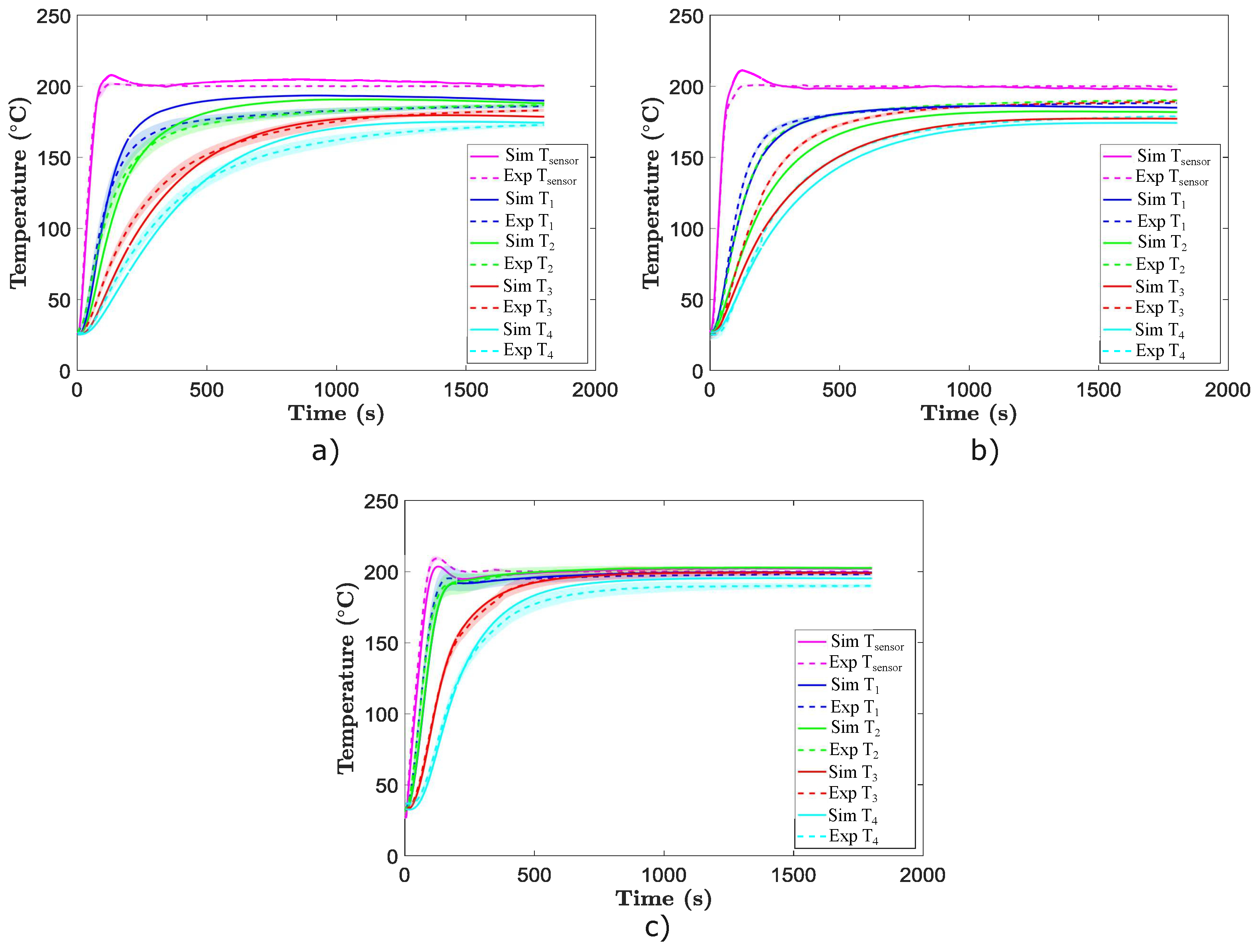
3.1. Experimental-Numerical Calibration of the Heat Loss Coefficients

The heat loss coefficients for the five calibrated models are presented in

Table 3. Heat loss coefficients: convective coefficients ($h_v^{conv}$ and $h_g^{conv}$), thermal conductance coefficients ($h_c^{vg}$, $h_c^{va}$ and $h_c^{ag}$) and emissivity coefficient ($ϵ$) for the five FE models, the two with the layer of air (Model I) and the three with the non-linear thermal conductance along the radius (Model II).

	Model I		Model II
	WMF	Schulte	WMF	Schulte	Steel Plate
$h_v^{conv}$ (W/m${}^2$K)	4	6	5.5	7	8
$h_g^{conv}$ (W/m${}^2$K)	4	4	5.5	5.5	4
$h_c^{vg}$ (W/m${}^2$K)	-	-	$h_c^{vg}$(r)	$h_c^{vg}$(r)	$h_c^{vg}$(r)
$h_c^{va}$ (W/m${}^2$K)	3000	3000	-	-	-
$h_c^{ag}$ (W/m${}^2$K)	3000	3000	-	-	-
$ϵ$	0.95	0.87	0.95	0.87	0.4

. Only the WMF and Schulte pans were developed in Model I because the steel plate is flat (Figure 2) and there is no layer of air to be modelled. Convective coefficients were optimised to reduce the mean absolute error (MAE) between the experimental and numerical temperatures. We obtained a convective coefficient of 8.0 W/m${}^2$K, similar to Sanz-Serrano et al. [11], which obtained a convective coefficient of 9.5 W/m${}^2$K using the difference finite method.

3.1.1. Model I: Modelling the Layer of Air between the Vessel and the Pan

Figure 5a,b show the WMF and Shulte heating processes, respectively. The dotted lines indicate the values obtained from the experimental tests whilst the continuous lines represent the computational results (see Figure 1b for the location of the thermal sensors). Shaded areas in the experimental tests are the standard deviations. Both numerical results of the surface thermocouples are within the experimental deviation.

The fitting between experimental and numerical results is good, although the experimental glass temperatures of the WMF pan heat up slightly faster than the simulated temperatures in the transient state (0–200 s). The temperatures in the steady state are practically the same.

Table 4. MAE of the three models with Model I. $T_{\mathit{sensor}}$, $T_1$, $T_2$, $T_3$ and $T_4$ are the thermocouples in Figure 1b. The units are ${}^{\circ }$C.

	${\mathit{T}}_{\mathit{s}\mathit{e}\mathit{n}\mathit{s}\mathit{o}\mathit{r}}$	${\mathit{T}}_1$	${\mathit{T}}_2$	${\mathit{T}}_3$	${\mathit{T}}_4$
WMF	2.63	4.63	5.36	3.33	6.75
Schulte	1.33	2.93	4.94	13.27	3.31

shows the MAEs between the numerical and experimental temperatures. The thermocouple placed in the centre ($T_4$) presented the highest error, 6.75 ${}^{\circ }$C.

On the other hand, during the whole heating process in the Schulte (Figure 5b), both the experimental and simulated results are similar (all MAEs are under 5 ${}^{\circ }$C) except for $T_3$, which differs more from the experimental temperature (MAE of 13.27 ${}^{\circ }$C). A misalignment of the thermal sensor or the vessel in the experimental tests might be one factor. This area has the largest concavity deviation and small variations can significantly influence the thermal contact conductance and thus the temperature.

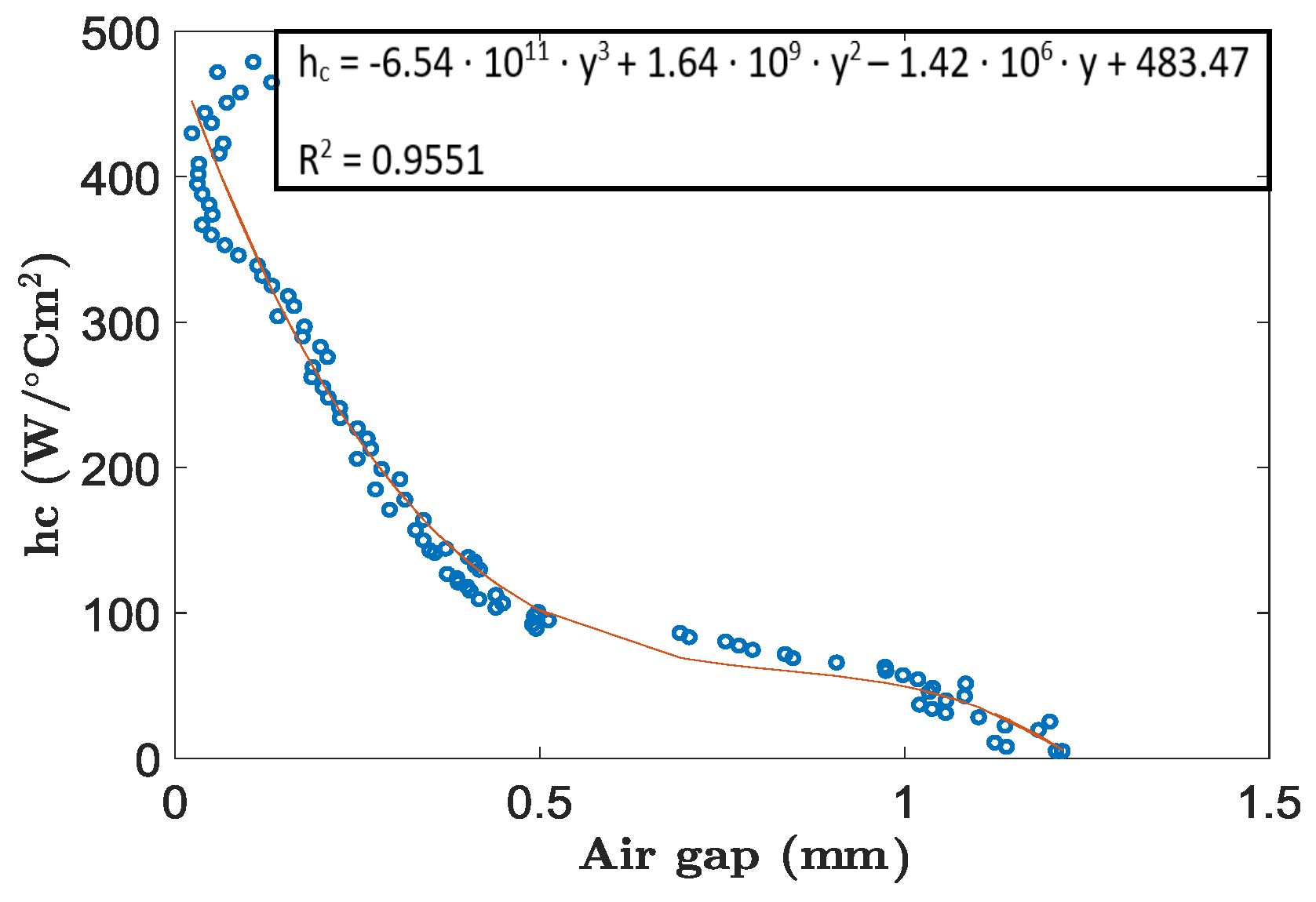
3.1.2. Model II: Fitting of the Nonlinear Thermal Conductance along the Radius

The equation that relates the thermal conductance coefficient and the air gap for the pans (WMF and Schulte) is shown in Figure 6. An iterative inverse analysis, such as in Paesa et al. [19], was performed, and it included several simulations of WMF with different variable thermal conductances along the radius. The optimal result was correlated with the concavity of the pan (see Figure 2), and thus, the following relationship, see Figure 6, was achieved. The WMF pan was used as reference vessel and the parameter fitting were also employed later for the Schulte pan simulations.

The results of the simulations are shown in Figure 7. The surface thermocouples of WMF and Schulte present very low MAEs of 3.09 ${}^{\circ }$C and 1.80 ${}^{\circ }$C, respectively (see

Table 5. MAE of the two models modelled with Model II. $T_{sensor}$, $T_1$, $T_2$, $T_3$ and $T_4$ are the thermocouples in Figure 1b. The units are ${}^{\circ }$C.

	${\mathit{T}}_{\mathit{s}\mathit{e}\mathit{n}\mathit{s}\mathit{o}\mathit{r}}$	${\mathit{T}}_1$	${\mathit{T}}_2$	${\mathit{T}}_3$	${\mathit{T}}_4$
WMF	3.09	9.45	6.69	3.77	5.65
Schulte	1.8	2.48	12.17	15.01	4.48
Steel plate	2.76	4.55	1.7	0.89	5.39

).

Regarding the glass thermocouples in the WMF (see Figure 7a), the experimental temperatures are slightly higher than the numerical temperatures in the transient state (approximately 0–200 s). For the Schulte pan, the experimental values are moderately higher than the simulated one during the whole cooking (see Figure 7b).

The heat conduction between the steel plate and the glass was initially considered as perfect as the plate is completely flat; however, the numerical results did not fit the experimental results. Thus, a thermomechanical analysis was performed to observe if there was a significant thermal deformation during the cooking that produced an input of air between the plate and the glass. It was noted that the concavity changes with increasing distance between the base vessel and the glass up to an axial displacement of 120 $\mathsf{\mu }$m (see Supplemental Data). Thus, $h_c^{vg}$ was modelled as piecewise as follows due to the thermomechanical analysis: from the centre until a radius of 10 cm is 50 W/m${}^2$K; from 20 to 50 cm of radii, 150 W/m${}^2$K; and the rest of the pan, 500 W/m${}^2$K. With this assumption, There was a clear correlation between the experimental and numerical temperatures, see Figure 7c.

3.1.3. Comparative between Model I and Model II

Both Model I and Model II show a good agreement with the experimental results. Overall, the results obtained for both the WMF and Schulte pans for Model II are slightly worse than those for Model I (see Table 4 and Table 5). If the concavity of the vessel is known, Model I might provide more accurate results. On the other side, Model II is indispensable for simulations where the concavity of the vessel is not known. However, it contains the tedious work of obtaining the variable thermal contact conductance by an inverse analysis.

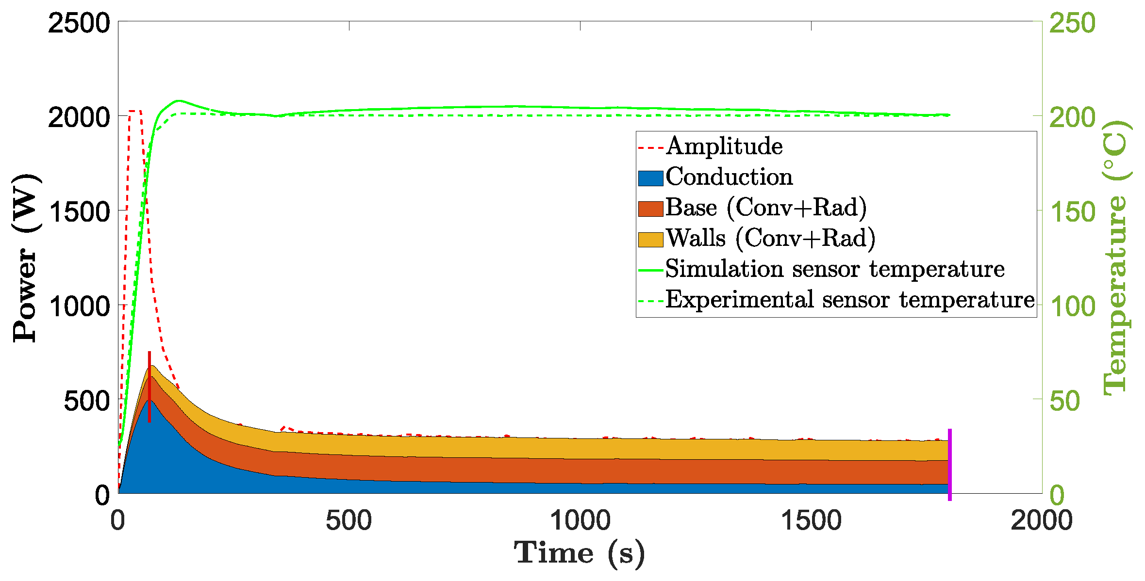
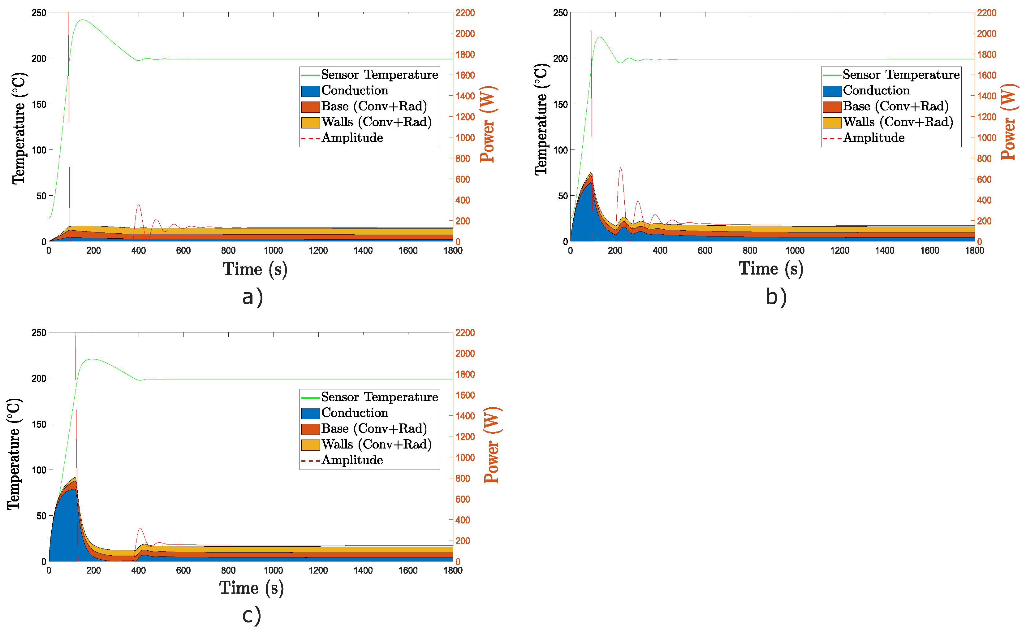
3.1.4. Heat Flux Analysis

The inbound energies, which are referred to as supplied power, and outbound energies, which are referred to as heat losses, of the WMF (using the Model II approach) are shown in Figure 8. The red dotted line represents the introduced power, the coloured areas refer to the heat losses during cooking, and the dotted and continuous green lines depict the experimental and simulation temperatures of the sensor, respectively. At the beginning of cooking, all the power is used as heat to warm up the vessel. When the temperature of the sensor reaches the target (200 ${}^{\circ }$C), the power decreases and maintains a constant value. The power of the steady state (approximately 400–1800 s) is converted into heat losses, mostly convection and radiation losses from the walls and the upper surface of the base (in yellow and orange).

The inbound and outbound energies of the Schulte and steel plate models are shown in the Supplemental Data. The heat losses of the three models at their maximum power level and at the end of cooking (red and pink line markers in Figure 8) are shown in

Table 6. Conduction, radiation and convection losses in the three vessels under investigation. The Schulte pan, that has the biggest concavity, presents the lowest conductivity losses during the transient state.

	Maximum Level			End of the Cooking
	WMF	Schulte	Steel Plate	WMF	Schulte	Steel Plate
Conduction (W)	496.7	122.4	546.6	49.6	14.9	46.8
Convection (W)	104.9	65.1	53.5	153.1	111.0	65.1
Radiation (W)	77.8	71.2	32.76	77.8	71.2	32.7

. In the transient state, conduction losses to the glass prevail above convection and radiation losses. However, in the steady state, convection losses become higher than the remaining ones. The results are consistent with Cabeza-Gil et al. [10] and Cadavid et al. [5].

The efficiency of the pans is calculated during the first 400 s as the energy used to heat up the vessel divided by the supplied energy as in Karunanithy and Shafer [9]. The efficiencies of the WMF, Schulte and steel plate are 79.95%, 82.5% and 74.18%, respectively. These values are consistent with those in Karunanithy and Shafer [9] and Villacis et al. [4], although the experimental setups were different and the experimental calculations can lead to some errors due to the approximation of the average temperature of the vessel. The energy necessary to heat up the solids during the 1800 s heating tests was 0.56 kWh, 0.38 kWh and 0.28 kWh for the WMF, Schulte and steel plate, respectively. These measurements were calculated as the temporal integration of the power supplied in the microsteel layer of the vessel.

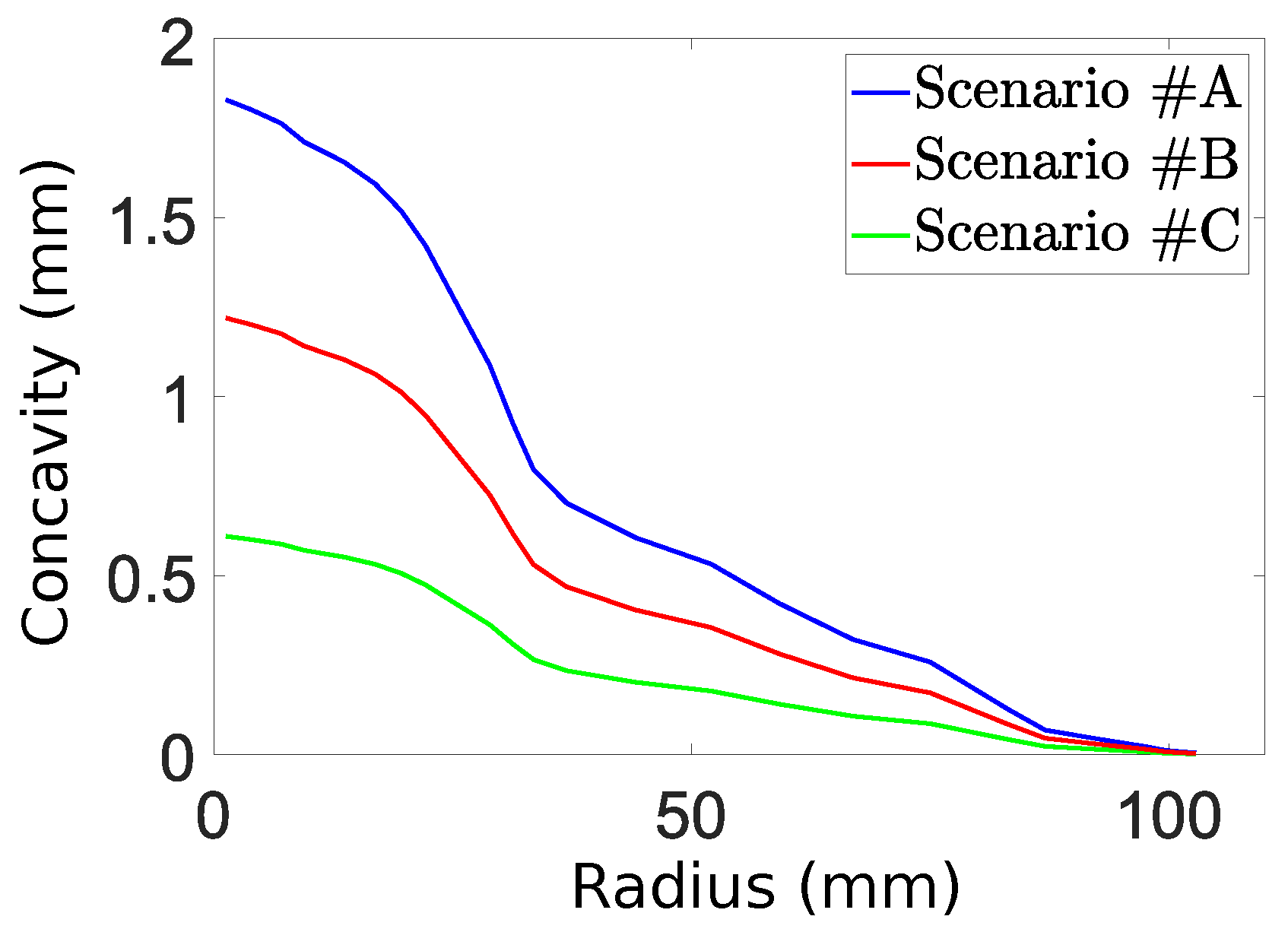
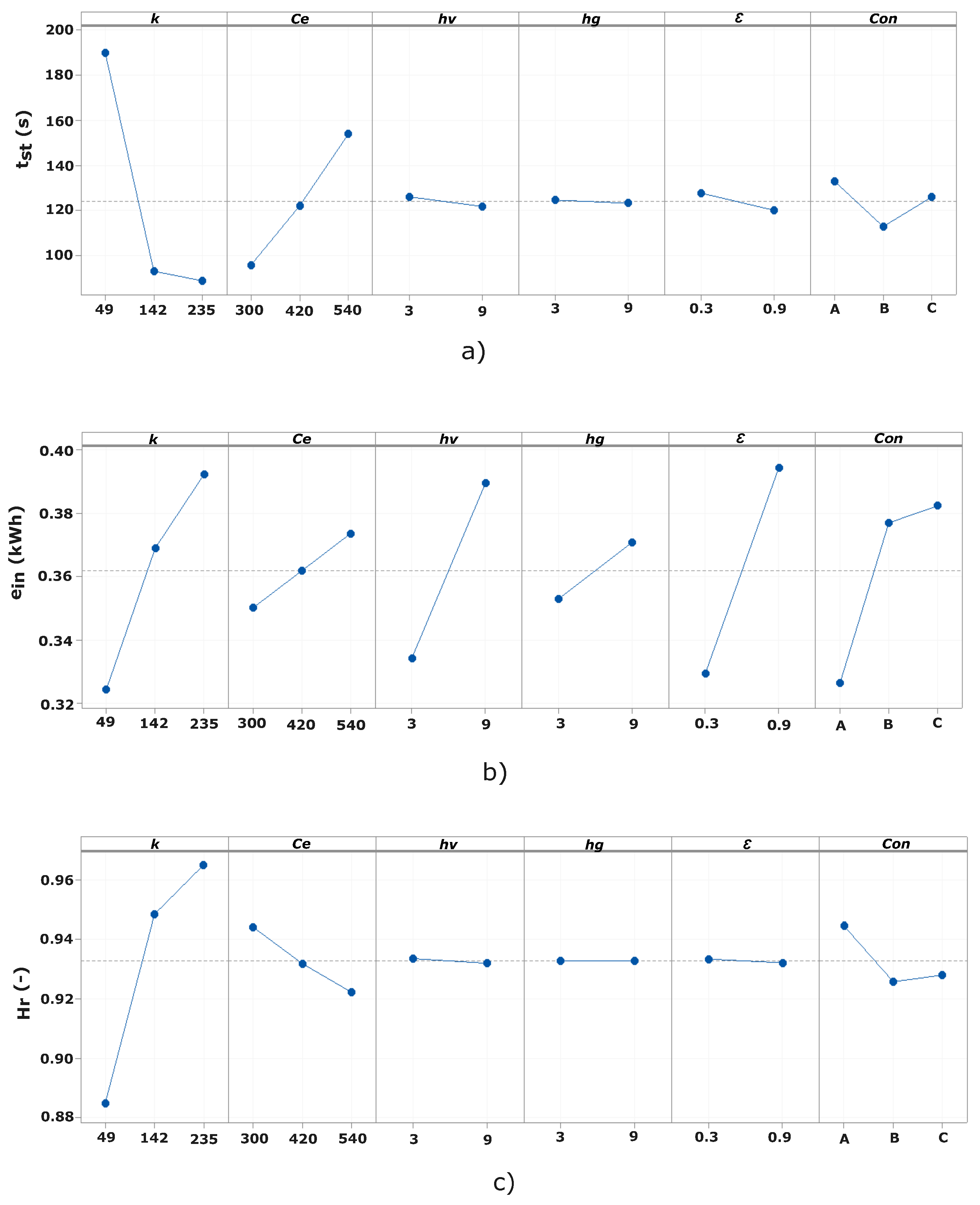
3.2. Design of Experiments (DoE)

In this section, the effects of the key parameters in the cooking and pan heating, namely, conductivity (k), specific heat ($c_e$), emissivity ($ϵ$), concavity ($Con$) of the vessel, and convective coefficients of the vessel ($h_v^{conv}$) and the glass ($h_g^{conv}$), are presented. The main responses in the heating tests, the time to reach steady state $t_{st}$, the introduced energy $E_{in}$ and the homogenisation along the radius in the second 60 of the cooking $H_r$, are shown through the main effects plots (see Figure 9). All results were supported by a Pareto analysis (see Supplemental Data).

Regarding the time to reach the steady state, as shown in Figure 9a, conductivity has the highest influence [20], and as it increases, the time to achieve the steady state decreases. Specific heat also influences $t_{st}$, and as it increases, more time is needed to heat the vessel. The rest of the parameters have little influence.

The most influential parameters in the supplied energy (Figure 9b) are the conductivity, vessel convective coefficient, emissivity and concavity. These results are consistent with Villacis et al. [4], Cadavid et al. [5], Newborough et al. [21] and Karunanithy and Shafer [9], who found that the efficiency of the pan depends on the pan composition and external surface emissivity.

We performed another analysis decreasing the cooking time to 400 s (see Supplemental Data), where the influence of the specific heat was not as high as expected. The effect of the supplied energy on the variable parameters was similar to that of the total lost energy during the whole cooking period (t = 1800 s); see Supplemental Data.

Lastly, concerning the temperature homogenisation along the radius after 1 min of cooking (Figure 9c), both convective coefficients and emissivity have no influence at all. The most important parameter is the conductivity, which is directly correlated with the temperature homogenisation.

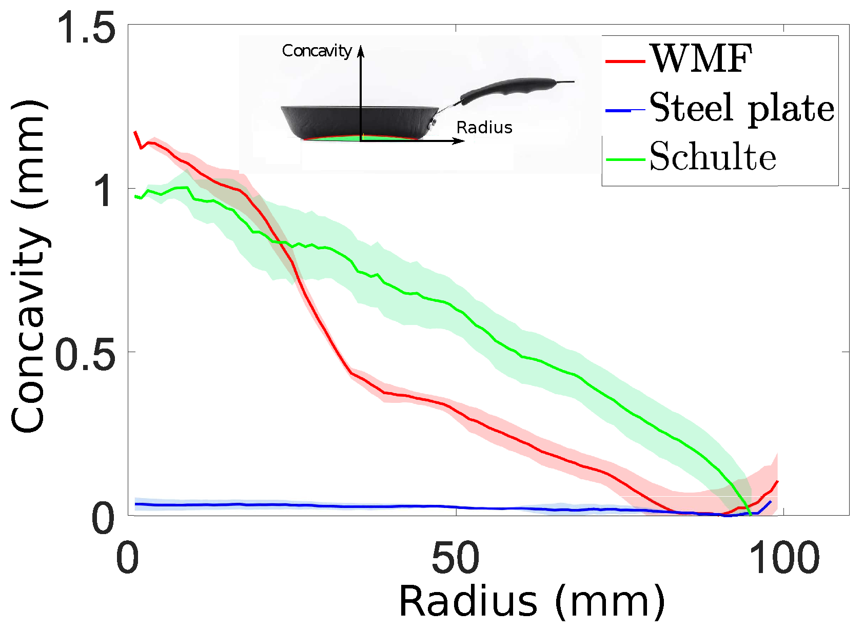
3.3. Influence of the Vessel Concavity

To better explain the effect of the vessel concavity, three heating scenarios were performed as examples with consistency in all of them, which means that they all have the same parameters except for concavity, which varied according to the levels in Table 2, which are represented in Figure 2.

The heat losses, amplitude of the power density and sensor temperature of the three cases are shown in Figure 10. Figure 10a corresponds to the highest concavity case, followed by Figure 10b,c with the lowest concavity. The conduction losses for the highest concavity case are minimum, which makes an overheating of the temperature sensor (because the sensor is placed at the center [10]). For the lowest concavity case, the conduction losses are the main losses at the beginning of the heating. After reaching the highest heat losses, the losses decrease rapidly as the glass has been heated; therefore, the temperature of the sensor decreases slowly because the pan loses less heat.

4. Conclusions

This study explored two novel approaches to model the thermal contact between the vessel and the cooktop, and thus achieving more realistic simulations. Once the numerical model was optimised, a design of experiments was performed to analyse the influence of the main parameters of the vessel during the cooking. The main conclusions of the study are as follows:

• The conductivity is the governing factor of the effect of the vessel in the cooking. When the vessel conductivity is high, it achieves the steady state and a better temperature homogeneity sooner. In contrast, the supplied energy is considerably higher. Thus, manufacturers should reach a compromise between being more energy effective and achieving a homogeneous temperature in the cooking surface in the shortest possible time.
• A more concave cooking vessel is more efficient, as the air layer between the pan base and the glass acts as insulation, reducing the heat losses of the vessel to the glass. The air gap should not be sufficiently large, as the magnetic field could lose efficiency.
• More than 80% of the heat losses during the transient state are due to the heat losses from the vessel to the glass.
• The main heat losses in the steady state are due to the convection and radiation.
• Both numerical approaches (Model I, including a layer of air and Model II, adding a variable thermal contact conductance) lead to similar results with MAEs lower than 5 K for the temperatures in the vessel and the glass. Model II adds the complexity of calibrating the variable thermal contact conductance.

References

1. Acero, J.; Burdio, J.; Barragan, L.; Navarro, D.; Alonso, R.; Ramon, J.; Monterde, F.; Hernandez, P.; Llorente, S.; Garde, I. Domestic Induction Appliances. IEEE Ind. Appl. Mag. 2010, 16, 39–47. [Google Scholar] [CrossRef]
2. Borg, S.; Kelly, N. The effect of appliance energy efficiency improvements on domestic electric loads in European households. Energy Build. 2011, 43, 2240–2250. [Google Scholar] [CrossRef]
3. Yohanis, Y.G. Domestic energy use and householders’ energy behaviour. Energy Policy 2012, 41, 654–665. [Google Scholar] [CrossRef]
4. Villacís, S.; Martínez, J.; Riofrío, A.; Carrión, D.; Orozco, M.; Vaca, D. Energy Efficiency Analysis of Different Materials for Cookware Commonly Used in Induction Cookers. Energy Procedia 2015, 75, 925–930. [Google Scholar] [CrossRef] [Green Version]
5. Cadavid, F.J.; Cadavid, Y.; Amell, A.A.; Arrieta, A.E.; Echavarría, J.D. Numerical and experimental methodology to measure the thermal efficiency of pots on electrical stoves. Energy 2014, 73, 258–263. [Google Scholar] [CrossRef]
6. Hannani, S.; Hessari, E.; Fardadi, M.; Jeddi, M. Mathematical modeling of cooking pots’ thermal efficiency using a combined experimental and neural network method. Energy 2006, 31, 2969–2985. [Google Scholar] [CrossRef]
7. Sedighi, M.; Dardashti, B. Finite element analysis of heat transfer in multi-layer cooking pots with emphasis on layer number. Int. J. Automot. Mech. Eng. 2015, 11, 2253–2261. [Google Scholar] [CrossRef]
8. Ayata, T.; Çavuşoğlu, A.; Arcaklioğlu, E. Predictions of temperature distributions on layered metal plates using artificial neural networks. Energy Convers. Manag. 2006, 47, 2361–2370. [Google Scholar] [CrossRef]
9. Karunanithy, C.; Shafer, K. Heat transfer characteristics and cooking efficiency of different sauce pans on various cooktops. Appl. Therm. Eng. 2016, 93, 1202–1215. [Google Scholar] [CrossRef]
10. Cabeza-Gil, I.; Calvo, B.; Grasa, J.; Franco, C.; Llorente, S.; Martínez, M. Thermal analysis of a cooking pan with a power control induction system. Appl. Therm. Eng. 2020, 180, 115789. [Google Scholar] [CrossRef]
11. Sanz-Serrano, F.; Sagues, C.; Llorente, S. Inverse modeling of pan heating in domestic cookers. Appl. Therm. Eng. 2016, 92, 137–148. [Google Scholar] [CrossRef] [Green Version]
12. Ogata, K. Modern Control Engineering; Prentice Hall: Hoboken, NJ, USA, 2010. [Google Scholar]
13. Hewitt, G.F.; Shires, G.L.; Bott, T.R. Process Heat Transfer; BHB: USA, 1994. Available online: https://www.begellhouse.com/ebook_platform/monograph/book/7daba87f6fb65d65.html (accessed on 10 February 2022).
14. Incropera, F.P.; DeWitt, D.P. Fundamentals of Heat and Mass Transfer, 8th ed.; John Wiley & Sons, Inc.: New York, NY, USA, 2017. [Google Scholar]
15. Acero, J.; Carretero, C.; Lope, I.; Alonso, R.; Burdio, J.M. FEA-Based Model of Elliptic Coils of Rectangular Cross Section. IEEE Trans. Magn. 2014, 50, 1–7. [Google Scholar] [CrossRef]
16. Lope, I.; Acero, J.; Carretero, C. Analysis and Optimization of the Efficiency of Induction Heating Applications with Litz-Wire Planar and Solenoidal Coils. IEEE Trans. Power Electron. 2016, 31, 5089–5101. [Google Scholar] [CrossRef] [Green Version]
17. Weissman, S.A.; Anderson, N.G. Design of experiments (DoE) and process optimization. A review of recent publications. Org. Process. Res. Dev. 2015, 19, 1605–1633. [Google Scholar] [CrossRef]
18. Seli, H.; Ismail, A.I.M.; Rachman, E.; Ahmad, Z.A. Mechanical evaluation and thermal modelling of friction welding of mild steel and aluminium. J. Mater. Process. Technol. 2010, 210, 1209–1216. [Google Scholar] [CrossRef]
19. Paesa, D.; Llorente, S.; Sagues, C.; Aldana, O. Adaptive Observers Applied to Pan Temperature Control of Induction Hobs. IEEE Trans. Ind. Appl. 2009, 45, 1116–1125. [Google Scholar] [CrossRef]
20. Lawless, Z.D.; Hobbs, M.L.; Kaneshige, M.J. Thermal conductivity of energetic materials. J. Energ. Mater. 2020, 38, 214–239. [Google Scholar] [CrossRef]
21. Newborough, M.; Probert, S.; Newman, M. Thermal performances of induction, halogen and conventional electric catering hobs. Appl. Energy 1990, 37, 37–71. [Google Scholar] [CrossRef]
Figure 1. (a) Representation of the systems that form Model I ( S 1 and S 2 are the same for Model II). S 1 corresponds to the system of the solid/pan, S 2 corresponds to the glass and S 3 corresponds to the air. The input heat is shown as red arrows, while outgoing heat is shown by blue arrows. Q ˙ p a n a i r and Q ˙ a i r g l a s s corresponds only to Model I. (b) Distribution of thermocouples in the vessel and the glass. The thermocouple (red) placed at the centre is used as input for the PI control ( T sensor ). Blue thermocouples are placed below the glass.
Mathematics 10 00802 g001
Figure 2. The mean and deviation concavity for each solid under investigation are depicted. The red line corresponds to the WMF, the green line to the Schulte and the blue line to the steel plate. The axis x = 0 is placed at the lowest geometric point of the vessel located in the periphery.
Mathematics 10 00802 g002
Figure 3. Vitroceramic glass is represented in orange, and the multilayer round WMF pan is represented in blue. Model I is modelled with the air (purple instance) between the glass and the pan, while Model II replaces the air by modelling the interaction between the vessel and glass by a variable thermal conductance coefficient along the radius.
Mathematics 10 00802 g003
Figure 4. Concavities of the three different scenarios. Scenario #A (blue line) corresponds to a larger concavity compared to scenario #B, the concavity measured to the WMF pan with the robot (red line). Scenario #C (green line) corresponds to a flatter concavity compared to scenario #B.
Mathematics 10 00802 g004
Figure 5. Temperatures of the surface and area under the glass from 0 to 1800 s for both the experimental test (dotted lines) and computational simulations (continuous lines) in Model I. (a) corresponds to the WMF pan and (b) to the Schulte pan.
Mathematics 10 00802 g005
Figure 6. Relation between the thermal conductance coefficient and the air gap. The relation and its equation, where y is the distance between the glass and the base of the pan, are shown graphically. The R-squared value of the regression model is also presented.
Mathematics 10 00802 g006
Figure 7. Temperatures of the surface and under the glass (see Figure 1b for location of the temperature sensors) from 0 to 1800 s for both experimental tests (dotted lines) and computational simulations (continuous lines) in Model II: (a) WMF pan, (b) Schulte pan and (c) steel plate.
Mathematics 10 00802 g007
Figure 8. Representation of the heat losses of computational Model II of the WMF (coloured areas), the amplitude of the power density introduced (red dotted line) and the experimental and simulation sensor temperatures (dotted and continuous green lines, respectively). The blue area corresponds to conduction losses between the base of the pan and the glass. The orange and yellow areas indicate the convection and radiation losses in the base and walls of the pan, respectively.
Mathematics 10 00802 g008
Figure 9. Main effects plot of conductivity (k), specific heat ( c e ), pan and glass convective coefficients ( h v and ( h g )), emissivity ( ϵ ) and concavity ( C o n ) for the responses: time to reach the steady state (a), supplied energy (b) and temperature homogenisation along the radius in the second 60 of the cooking (c). The units of the parameters are conductivity (W/mK); specific heat (J/kgK); convective coefficients (W/m 2 K); emissivity (-); and concavity (-).
Mathematics 10 00802 g009
Figure 10. Temperature of the sensor (green continuous line), amplitude of the power density (red dotted line) and losses (coloured areas) of three WMF pans that only differ on its concavity, case #A (a), case #B (b) and case #C (c) (see Figure 4). The yellow area represents convective and radiation losses of the walls, the orange area represents convective and radiation losses of the base of the pan, and the blue area represents conduction losses to the glass.
Mathematics 10 00802 g010