An Efficient Algorithm to Compute the Linear Complexity of Binary Sequences

Abstract

Binary sequences are algebraic structures currently used as security elements in Internet of Things devices, sensor networks, e-commerce, and cryptography. In this work, a contribution to the evaluation of such sequences is introduced. In fact, we present a novel algorithm to compute a fundamental parameter for this kind of structure: the linear complexity, which is related to the predictability (or non-predictability) of the binary sequences. Our algorithm reduced the computation of the linear complexity to just the addition modulo two (XOR logic operation) of distinct terms of the sequence. The performance of this procedure was better than that of other algorithms found in the literature. In addition, the amount of required sequence to perform this computation was more realistic than in the rest of the algorithms analysed. Tables, figures, and numerical results complete the work.

1. Introduction

The Internet is rapidly evolving, making possible the connectivity among any kinds of devices and giving rise to the Internet of Things (IoT) [1,2]. The IoT is based on all the applications and possibilities provided by the devices of daily use such as mobile phones, televisions, refrigerators, etc., to improve people’s lives and business environments. Nevertheless, the need to secure the interconnection of all these devices soon arose. This task is not easy, since the vast majority of IoT devices are not manufactured nor designed with safety in mind. Moreover, these devices are very different from each other, and security must be adapted to distinct models, types, and technical characteristics.

The security of an IoT network involves different techniques, i.e., blockchain, trust management [3,4,5], as well as cryptographic mechanisms. Cryptographic security is needed to prevent users from losing data and to avoid risks related to the inappropriate use of passwords. Many designs providing cryptographic security are based on true random numbers, but their generation is a complex task [6,7]. Some popular random noise algorithms are somehow imperfect, showing defects that make them vulnerable and predictable, which in cryptographic terms is a real concern. Some weaknesses are never found, at least publicly, and create a false sense of security in the community of users. The devices in which faults are detected are those with the most flagrant glitches or those that are most popular, e.g.: (1) the algorithm A5 in GSM mobile communications cryptanalysed in [8,9]; (2) the J3Gen generator for low-cost passive RFID tags; (3) the generator RC4 for encrypting Internet traffic that was also cryptanalysed in [10,11]. In brief, it is difficult to design a true random number generator that can provide a strong cryptographic basis for system security, especially for IoT devices; see [12,13].

Pseudo-Random Number Generators (PRNGs) are deterministic algorithms [14,15] used to produce random number sequences for cryptographic applications, such as digital signatures, the generation of nonces or keys, etc. These applications require some statistical properties in their output sequences such as a large period and linear complexity, low auto-correlation, wide dimensional distribution, the uniformity of the distribution for large quantities of generated numbers, etc. The interested reader is referred to [16] (Chapter 2).

Binary sequences generated by maximal-period Linear Feedback Shift Registers (LFSRs), i.e., PN-sequences [17], have been extensively used in many and diverse applications such as e-commerce, mobile wireless communications, digital broadcasting, and cryptography (stream ciphers) [18,19]. In order to ensure their cryptographic use, it is required to remove the linearity inherent to the PN-sequences. LFSRs play an important part in the design of cryptographic PNRGs [20,21]. Among the most popular families of cryptographic sequence generators based on PN-sequences, we can highlight the irregular decimation-based generators. The method of irregularly decimating the output sequences of LFSRs [22] generates powerful PNRGs that produce, in turn, sequences with good cryptographic properties such as: long periods, large linear complexity, two-valued auto-correlation properties, good distribution of zeros and ones along the sequence, etc. One of the most important generators in this family is the Generalized Self-Shrinking Generator (GSSG) [23]. This generator is fast, easy to implement, and generates good cryptographic sequences [24], so it is appropriate for low-cost applications.

In this paper, we present a contribution to security whose significance is limited to cryptographic mechanisms. In fact, our proposal is an algorithm that computes the linear complexity of sequences with a period of a power of two. The technique herein presented uses Hadamard matrices [25] and the B-representation of sequences proposed in [26,27]. Our algorithm was much more efficient than the other ones proposed in the literature [26,28,29,30], and the required amount of sequence to perform this computation was also more realistic.

Furthermore, besides being faster and requiring less intercepted bits of the sequence, the importance of this algorithm relies on the fact that it is especially efficient for families of sequences with an upper bound on the parameter’s linear complexity, i.e, the sequences generated by the Generalized Self-Shrinking Generator (GSSG) [23].

Our contributions can be enumerated as follows: (1) some basic concepts needed to understand the rest of the paper are introduced (Section 2); (2) we recall the concept of B-representation and establish a relation between this representation of sequences and the Hadamard matrices (Section 3); (3) we propose a novel method of computing the linear complexity of sequences with a period of a power of two and apply it to generalized sequences in Section 4 and Section 5, respectively; (4) we discuss (Section 6) the advantages of our method when compared with the other ones; (5) the paper ends (Section 7) with some important remarks concerning our results.

2. Basic Concepts and Generalities

In this section, we introduce different concepts and structures that are used systematically throughout the work.

2.1. Linear Feedback Shift Registers

Let ${\mathbb{F}}_2=\{0,1\}$ be the Galois field of two elements. Consider ${\left\{u_i\right\}}_{i\ge 0}=\{u_0,u_1,u_2,\dots \}$ a binary sequence with $u_i\in {\mathbb{F}}_2$, for $i=0,1,2,\dots$ We say that the sequence ${\left\{u_i\right\}}_{i\ge 0}$ is periodic if there exists an integer T, called the period, such that $u_{i+T}=u_i$, for all $i\ge 0$. In the sequel, all the sequences considered are binary sequences, and the symbol + denotes the Exclusive-OR (XOR) logic operation.

Let r be a positive integer, and let $a_1,a_2,a_3,\dots ,a_r$ be constant coefficients with $a_j\in {\mathbb{F}}_2$, for $j=1,2,\dots ,r$. A binary sequence ${\left\{u_i\right\}}_{i\ge 0}$ satisfying the relation:

$$u_{i+r}=a_1{u}_{i+r-1}+a_2{u}_{i+r-2}+a_3{u}_{i+r-3}+\cdots +a_{r-1}{u}_{i+1}+a_r{u}_i,i\ge 0,$$

(1)

is called an r-th order linear recurring sequence in ${\mathbb{F}}_2$. The terms $\{u_0,u_1,\dots ,$$u_{r-1}\}$ are referred to as the initial terms and define uniquely the construction of the sequence.

A relation of the form given by Equation (1) is called an r-th order linear recurrence relationship.

The monic polynomial:

$$p\left(x\right)=x^r+a_1{x}^{r-1}+a_2{x}^{r-2}+a_3{x}^{r-3}+\cdots +a_{r-1}x+a_r\in {\mathbb{F}}_2\left[x\right]$$

is called the characteristic polynomial of the linear recurring sequence and ${\left\{u_i\right\}}_{i\ge 0}$ is said to be generated by $p\left(x\right)$.

We can obtain linear recurring sequences through Linear Feedback Shift Registers (LFSRs) [17]. In fact, an LFSR can be defined as an electronic device with r interconnected memory cells (or stages) with binary content. At every clock pulse, the binary element of each stage is shifted to the adjacent stage, as well as a new element is computed through the linear feedback to fill the empty stage (see Figure 1). We say that the LFSR has the maximal length if the characteristic polynomial of the linear recurring sequence is primitive. In this case, its output sequence is called the Pseudo-Noise sequence (PN-sequence), and its period is $T=2^r-1$ with $2^{r-1}$ ones and $2^{r-1}-1$ zeros; see [17].

The linear complexity of a sequence ${\left\{u_i\right\}}_{i\ge 0}$, denoted by $LC$, is defined as the length of the shortest LFSR that generates such a sequence or, equivalently, as the lowest-order linear recurrence relationship that generates such a sequence.

In cryptographic applications, the linear complexity must be as large as possible. The expected value is approximately half the period $LC\simeq T/2$ (see [31]).

2.2. The Generalized Self-Shrinking Generator

Consider a PN-sequence ${\left\{u_i\right\}}_{i\ge 0}$ obtained from a maximal-length LFSR with L stages and an L-dimensional binary vector $\mathcal{G}=[g_0,g_1,g_2,...,g_{L-1}]\in {\mathbb{F}}_2^L$, and let ${\left\{v_i\right\}}_{i\ge 0}$ be the sequence defined as:

$$v_i=g_0{u}_i+g_1{u}_{i-1}+g_2{u}_{i-2}+\cdots +g_{L-1}{u}_{i-L+1}\mathrm{for}i\ge 0.$$

(2)

Next, we define a decimation rule to generate a new sequence ${\left\{s_j\right\}}_{j\ge 0}$ as follows:

$$\left\{\begin{array}{cc}If{u}_i=1,\hfill & \mathrm{then}{s}_j=v_i;\hfill \\ If{u}_i=0,\hfill & \mathrm{then}{v}_i\mathrm{is}\mathrm{discarded}.\hfill \end{array}\right.$$

The sequence ${\left\{s_j\right\}}_{j\ge 0}$, denoted by $S\left(\mathcal{G}\right)$, is called the generalized self-shrunken sequence, GSS-sequence, or simply generalized sequence associated with $\mathcal{G}$; see [23]; the sequence generator is called the Generalized Self-Shrinking Generator (GSSG). The set of sequences $\mathcal{S}=\left\{S\left(\mathcal{G}\right)|\mathcal{G}\in {\mathbb{F}}_2^L\right\}$ is called the family of generalized sequences based on the PN-sequence ${\left\{u_i\right\}}_{i\ge 0}$. It is worth noticing that the period of any generalized sequence is a divisor of $2^{L-1}$ (as $2^{L-1}$ is the number of ones in the PN-sequence), and the linear complexity satisfies [29]:

$$2^{L-2}<LC\le 2^{L-1}-(L-2).$$

(3)

In order to analyse more properties of this generator, the interested reader is referred to [22,23,27,32].

From now on, we consider a sequence with the notation ${\left\{u_i\right\}}_{i\ge 0}$ or $\left\{u_i\right\}$, indistinctly.

2.3. Binomial Sequences

The binomial number $\left(\genfrac{}{}{0pt}{}{n}{i}\right)$ represents the coefficient corresponding to the power $x^i$ in the algebraic expansion of the polynomial ${(1+x)}^n$. For every integer $n\ge 0$, we know that $\left(\genfrac{}{}{0pt}{}{n}{0}\right)=1$, while $\left(\genfrac{}{}{0pt}{}{n}{i}\right)=0$ for $i>n$. Now, the binomial sequences are introduced as follows.

Definition 1.

Given a fixed integer $k\ge 0$, the k-th binomial sequence is given by:

$${\left\{\left(\genfrac{}{}{0pt}{}{n}{k}\right)\right\}}_{n\ge 0}=\left\{\begin{array}{cc}0,\hfill & ifn<k,\hfill \\ \left(\genfrac{}{}{0pt}{}{n}{k}\right)mod2,\hfill & ifn\ge k.\hfill \end{array}\right.$$

Table 1. The first 8 binomial coefficients $\left(\genfrac{}{}{0pt}{}{n}{k}\right)$$(0\le k<8)$ and their binomial sequences $\left\{\left(\genfrac{}{}{0pt}{}{n}{k}\right)\right\}$, periods, and linear complexities.

Binomial Coeff.	Binomial Sequences $\left\{\left(\genfrac{}{}{0pt}{}{\mathit{n}}{\mathit{k}}\right)\right\}$	Period	LC
$\left(\genfrac{}{}{0pt}{}{n}{0}\right)$	$11111111\dots$	1	1
$\left(\genfrac{}{}{0pt}{}{n}{1}\right)$	$01010101\dots$	2	2
$\left(\genfrac{}{}{0pt}{}{n}{2}\right)$	$00110011\dots$	4	3
$\left(\genfrac{}{}{0pt}{}{n}{3}\right)$	$00010001\dots$	4	4
$\left(\genfrac{}{}{0pt}{}{n}{4}\right)$	$00001111\dots$	8	5
$\left(\genfrac{}{}{0pt}{}{n}{5}\right)$	$00000101\dots$	8	6
$\left(\genfrac{}{}{0pt}{}{n}{6}\right)$	$00000011\dots$	8	7
$\left(\genfrac{}{}{0pt}{}{n}{7}\right)$	$00000001\dots$	8	8

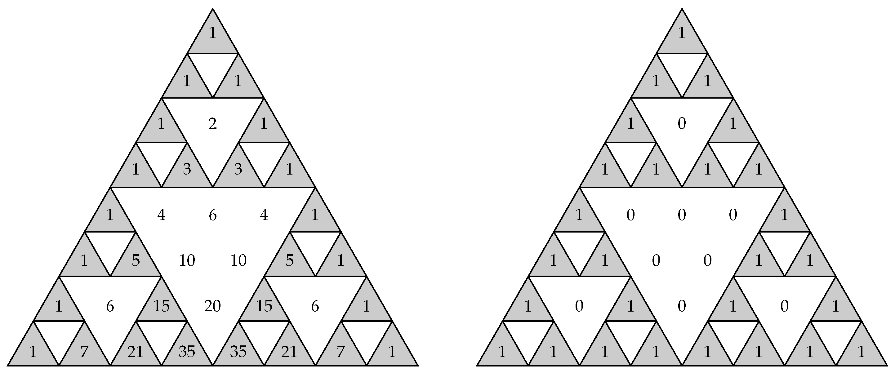
shows the first eight binomial coefficients, as well as the first eight binomial sequences with their corresponding periods and linear complexities. Moreover, recall that the binomial sequences are just shifted versions (starting in the first one) of the successive diagonals of Sierpinski’s triangle reduced modulo two, as depicted in Figure 2.

In the following, we recall some results about the period and the structure of the binomial sequences.

Proposition 1

([26], Proposition 3). Given the binomial sequence $\left\{\left(\genfrac{}{}{0pt}{}{n}{2^L+k}\right)\right\}$, with $0\le k<2^L$, we have that:

(a) 

The period of such a sequence is $T=2^{L+1}$;

(b) 

The period of such a sequence has the following structure:

$${\left\{\left(\genfrac{}{}{0pt}{}{n}{2^L+k}\right)\right\}}_{0\le n<2^{L+1}} = \left\{\begin{array}{cc}0\hfill & if0\le n<2^L+k,\hfill \\ \left(\genfrac{}{}{0pt}{}{n}{k}\right)\hfill & if{2}^L+k\le n<2^{L+1}.\hfill \end{array}\right.$$

Corollary 1

([26], Corollary 4). The binomial sequences of the form $\left\{\left(\genfrac{}{}{0pt}{}{n}{2^L}\right)\right\}$, $(L=0,1,2,\dots )$ have period $T=2^{L+1}$ and the following structure:

$${\left\{\left(\genfrac{}{}{0pt}{}{n}{2^L}\right)\right\}}_{0\le n<2^{L+1}} = \left\{\begin{array}{c}0If0\le n<2^L;\hfill \\ 1If{2}^L\le n<2^{L+1}.\hfill \end{array}\right.$$

Corollary 2

([26], Corollary 5). The binomial sequences of the form $\left\{\left(\genfrac{}{}{0pt}{}{n}{2^L}\right)\right\}$$(L=0,1,2,\dots )$ are balanced, i.e, they contain the same number of ones and zeros.

The proofs and more properties of such sequences can be found in [26].

Remark 1.

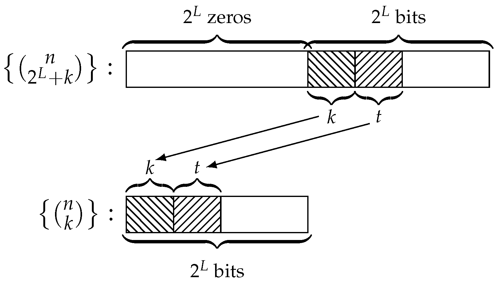
The binomial sequences have the following structure:

$$\begin{array}{cc}\hfill \left\{\left(\genfrac{}{}{0pt}{}{n}{2^L}\right)\right\}:& \underset{2^L\mathit{zeros}}{\underbrace{00\dots 0}}\underset{2^L\mathit{ones}}{\underbrace{11\dots 1}}\hfill \\ \hfill \left\{\left(\genfrac{}{}{0pt}{}{n}{2^L+k}\right)\right\}:& \underset{2^L\mathit{zeros}}{\underbrace{00\dots 0}}\underset{\begin{array}{c}\hfill \begin{array}{c}\mathit{the}\mathit{first}{2}^L\mathit{terms}\\ \mathit{of}\left\{\left(\genfrac{}{}{0pt}{}{n}{k}\right)\right\}\end{array}\end{array}}{\underbrace{\dots \dots \dots \dots }}\hfill \end{array}$$

See the Figure 3 for more details. The following example illustrates the previous results.

Example 1.

The binomial sequence $\left\{\left(\genfrac{}{}{0pt}{}{n}{4}\right)\right\}$ has period eight and is composed of four consecutive zeros followed by four consecutive ones:

$$\left\{\left(\genfrac{}{}{0pt}{}{n}{4}\right)\right\}:00001111$$

The binomial sequence $\left\{\left(\genfrac{}{}{0pt}{}{n}{7}\right)\right\}=\left\{\left(\genfrac{}{}{0pt}{}{n}{4+3}\right)\right\}$ has also period eight and is composed of four consecutive zeros followed by the first four bits of $\left\{\left(\genfrac{}{}{0pt}{}{n}{3}\right)\right\}:$

$$\left\{\left(\genfrac{}{}{0pt}{}{n}{7}\right)\right\}:0000\underset{\left\{\left(\genfrac{}{}{0pt}{}{n}{3}\right)\right\}}{\underbrace{0001}}$$

Theorem 1.

The linear complexity of the binomial sequence $\left\{\left(\genfrac{}{}{0pt}{}{n}{k}\right)\right\}$ is $k+1$.

Notice that, as a consequence of Theorem 1, the linear complexity of any binomial sequence is immediate. Furthermore, in the following sections, we will see that any sequence of a period of a power of two can be expressed as a sum (modulo two) of binomial sequences. As a result, it is easy to compute the linear complexity of such sequences by just observing the binomial sequence of a greater degree in the binomial decomposition [26].

2.4. Construction of Binomial Matrices from Binomial Sequences

In this subsection, we introduce the concept of the binomial matrix, which is closely related with the binomial sequences and Sierpinski’s triangle.

Definition 2.

Let t be a non-negative integer. We define the binomial matrix$H_t$ as the binary Hadamard matrix of size $2^t\times 2^t$ constructed as follows: $H_0=\left[1\right]$, for $t=0$, and:

$$H_t=\left[\begin{array}{cc}{H}_{t-1}& H_{t-1}\\ 0_{t-1}& H_{t-1}\end{array}\right],$$

for $t>0$, with $0_{t-1}$ the $2^{t-1}\times 2^{t-1}$ null matrix.

In general, any binomial matrix $H_t$ can be easily constructed from binomial sequences as follows:

• Its rows correspond to the first $2^t$ bits of the first $2^t$ binomial sequences, that is,

  $$H_t=\left[\begin{array}{c}\left\{\left(\genfrac{}{}{0pt}{}{n}{0}\right)\right\}\\ \\ \left\{\left(\genfrac{}{}{0pt}{}{n}{1}\right)\right\}\\ ⋮\\ \left\{\left(\genfrac{}{}{0pt}{}{n}{2^t-2}\right)\right\}\\ \\ \left\{\left(\genfrac{}{}{0pt}{}{n}{2^t-1}\right)\right\}\end{array}\right]=\left[\begin{array}{ccccccccccc}1& 1& 1& 1& 1& 1& \dots & 1& 1& 1& 1\\ 0& 1& 0& 1& 0& 1& \dots & 0& 1& 0& 1\\ ⋮& ⋮& ⋮& ⋮& ⋮& ⋮& & ⋮& ⋮& ⋮& ⋮\\ 0& 0& 0& 0& 0& 0& \dots & 0& 0& 1& 1\\ 0& 0& 0& 0& 0& 0& \dots & 0& 0& 0& 1\end{array}\right];$$
• Its columns correspond to the first $2^t$ bits of shifted versions of the first $2^t$ binomial sequences starting in their first one, i.e., the columns of $H_t$ are the diagonals of Sierpinski’s triangle (see Figure 2):

  $$H_t=\left[\begin{array}{ccccc}{\left\{\left(\genfrac{}{}{0pt}{}{n}{2^t-1}\right)\right\}}^{*}& {\left\{\left(\genfrac{}{}{0pt}{}{n}{2^t-1}\right)\right\}}^{*}& \dots & {\left\{\left(\genfrac{}{}{0pt}{}{n}{1}\right)\right\}}^{*}& {\left\{\left(\genfrac{}{}{0pt}{}{n}{0}\right)\right\}}^{*}\end{array}\right]=\left[\begin{array}{ccccc}1& 1& \dots & 1& 1\\ 0& 1& \dots & 0& 1\\ 0& 0& \dots & 1& 1\\ 0& 0& \dots & 0& 1\\ ⋮& ⋮& & ⋮& ⋮\\ 0& 0& \dots & 1& 1\\ 0& 0& \dots & 0& 1\end{array}\right].$$

In the previous expression, we denoted by ${\left\{\left(\genfrac{}{}{0pt}{}{n}{k}\right)\right\}}^{*}$ the shifted version of the binomial sequence $\left\{\left(\genfrac{}{}{0pt}{}{n}{k}\right)\right\}$ starting in the first one $(k=0,\dots ,2^t-1)$.

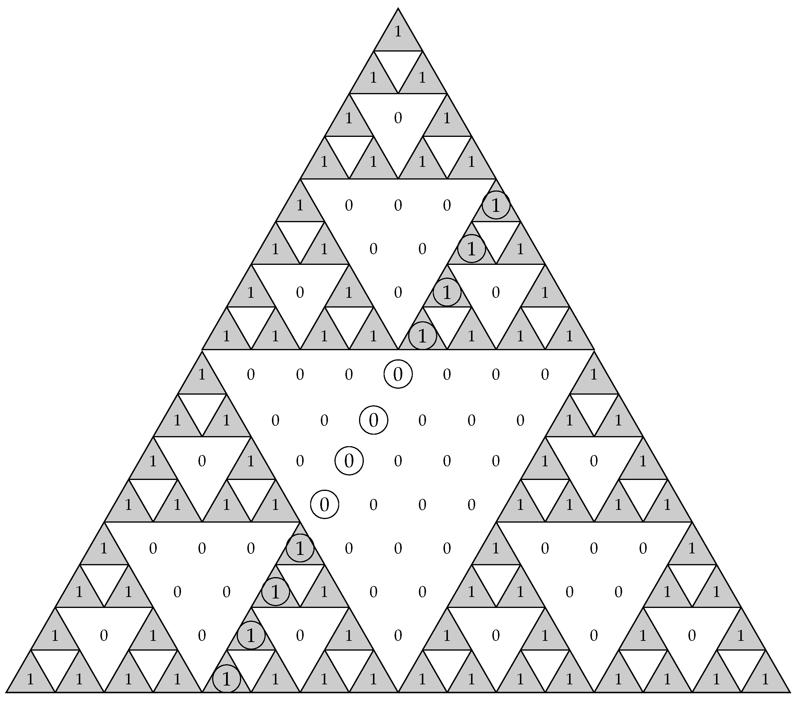
As we said before, the diagonals of the Sierpinski triangle correspond to the columns of the Hadamard matrix, and at the same time, they are shifted versions of the binomial sequences, that is the rows of the same matrix. See, for example, Figure 4. The circled diagonal corresponds to the shifted version ${\left\{\left(\genfrac{}{}{0pt}{}{n}{4}\right)\right\}}^{*}$ of the binomial sequence $\left\{\left(\genfrac{}{}{0pt}{}{n}{4}\right)\right\}$. Notice that the sequence $\left\{\left(\genfrac{}{}{0pt}{}{n}{4}\right)\right\}$ corresponds to the fourth row of $H_t$, and the circled diagonal corresponds to the $(2^t-5)$-th column of $H_t$, for t sufficiently large. In general, the sequence $\left\{\left(\genfrac{}{}{0pt}{}{n}{k}\right)\right\}$ corresponds to the k-th row of $H_t$, and the shifted version ${\left\{\left(\genfrac{}{}{0pt}{}{n}{k}\right)\right\}}^{*}$ (that is, the k-th diagonal of Sierpinski’s triangle) corresponds to the $(2^t-k-1)$-th column of $H_t$, for t sufficiently large.

In brief, there is a close relation among binomial sequences, diagonals of Sierpinski’s triangle, and binary Hadamard matrices.

3. B-Representation

The binomial representation (B-representation) of binary sequences was first introduced in [26]. In fact, every binary sequence $\left\{s_n\right\}$ whose period T is a power of two, that is $T=2^t$, can be expressed as a linear combination of binomial sequences as follows:

$$\left\{s_n\right\}=\sum _{i=0}^{2^t-1}{c}_i\left\{\left(\genfrac{}{}{0pt}{}{n}{i}\right)\right\},$$

(4)

where t is a non-negative integer, $\left\{\left(\genfrac{}{}{0pt}{}{n}{i}\right)\right\}$ is the i-th binomial sequence, and the coefficients $c_i\in {\mathbb{F}}_2$, for $(i=0,1,\dots ,2^t-1)$. The above equation is the B-representation of the sequence $\left\{s_n\right\}$.

Let $imax$ be an integer in the interval $(0\le imax\le 2^t-1)$ such that the coefficient $c_{imax}$ of the B-representation satisfies:

$c_{imax}\ne 0$ while $c_i=0$ for all index i in the range $(imax<i\le 2^t-1)$.

The coefficient $c_{imax}$ and the B-representation provide us with information about two fundamental parameters of the sequence, the period and the linear complexity:

• Period of $\left\{s_n\right\}$ in terms of the B-representation: As a consequence of Proposition 1, it is possible to prove that the period T of the sequence $\left\{s_n\right\}$ is the period of the binomial sequence $\left\{\left(\genfrac{}{}{0pt}{}{n}{imax}\right)\right\}$, since the period of the sequence is the greatest period of the binomial sequences included in its B-representation (see ([26], Proposition 3));
• Linear complexity of $\left\{s_n\right\}$ in terms of the B-representation: As a consequence of Theorem 1, the linear complexity of the sequence $\left\{s_n\right\}$ is the linear complexity of the binomial sequence $\left\{\left(\genfrac{}{}{0pt}{}{n}{imax}\right)\right\}$ (see ([26], Corollary 14)), that is:

  $$LC=imax+1.$$

  (5)

Fixing a linear complexity $LC$, the period T of the corresponding sequence is uniquely determined. Nevertheless, fixing a period T, there exist distinct sequences with such a period, but with different values of their linear complexities, as we can observe in Table 1.

Due to the particular structure of the binomial sequences, we can reformulate the binomial representation of $\left\{s_n\right\}$ given in Equation (4) and convert it into a matrix equation using the binomial matrix $H_t$.

Theorem 2.

Consider the B-representation of a sequence $\left\{s_n\right\}$ of period $T=2^t$, with t a non-negative integer, and let $H_t$ be the binomial matrix of size $2^t\times 2^t$. Then,

$$(s_0,s_1,\dots ,s_{2^t-1})=(c_0,c_1,\dots ,c_{2^t-1})·H_{t}mod2,$$

where the vector $(s_0,s_1,\dots ,s_{2^t-1})$ corresponds to the $2^t$ successive terms of the sequence $\left\{s_n\right\}$ and $(c_0,c_1,\dots ,c_{2^t-1})$ are the coefficients that weight the binomial sequences in (4).

Proof. 

From the B-representation of $\left\{s_n\right\}$ given in Expression (4), we have that:

$$\begin{array}{cccccccccccccccc}& c_0& ·& \{1& 1& 1& 1& 1& 1& 1& 1& \dots & 1& 1& 1& 1\}\\ & c_1& ·& \{0& 1& 0& 1& 0& 1& 0& 1& \dots & 0& 1& 0& 1\}\\ & c_2& ·& \{0& 0& 1& 1& 0& 0& 1& 1& \dots & 0& 0& 1& 1\}\\ & c_3& ·& \{0& 0& 0& 1& 0& 0& 0& 1& \dots & 0& 0& 0& 1\}\\ & ⋮& & ⋮& ⋮& ⋮& ⋮& ⋮& ⋮& ⋮& ⋮& & ⋮& ⋮& ⋮& ⋮\\ & c_{2^t-4}& ·& \{0& 0& 0& 0& 0& 0& 0& 0& \dots & 1& 1& 1& 1\}\\ & c_{2^t-3}& ·& \{0& 0& 0& 0& 0& 0& 0& 0& \dots & 0& 1& 0& 1\}\\ & c_{2^t-2}& ·& \{0& 0& 0& 0& 0& 0& 0& 0& \dots & 0& 0& 1& 1\}\\ +& c_{2^t-1}& ·& \{0& 0& 0& 0& 0& 0& 0& 0& \dots & 0& 0& 0& 1\}\\ \left\{s_n\right\}& =& & \{s_0& s_1& s_2& s_3& s_4& s_5& s_6& s_7& \dots & s_{2^t-4}& s_{2^t-3}& s_{2^t-2}& s_{2^t-1}\}\end{array}$$

where $s_k$, the k-th term of the sequence $\left\{s_n\right\}$, is the bitwise XOR operation of the k-th term of each binomial sequence, notated $\left(\genfrac{}{}{0pt}{}{k}{i}\right)$, multiplied by its corresponding coefficient $c_i$$(i=0,1,\dots ,2^t-1)$, that is:

$$s_k=\sum _{i=0}^{2^t-1}{c}_i\left(\genfrac{}{}{0pt}{}{k}{i}\right).$$

Thus, in matrix form, the previous representation can be expressed as:

$$(s_0,s_1,\dots ,s_{2^t-1})=(c_0,c_1,\dots ,c_{2^t-1})·H_t\mathit{mod}2.$$

(6)

□

An useful property of the Hadamard matrices is described as follows:

Lemma 1.

The inverse of a binomial matrix $H_t$ is the matrix itself, i.e., it is an idempotent matrix.

Proof. 

We proceed by induction. We have that $H_2^2=I_2$, where $I_2$ is the identity matrix of size $2\times 2$. Suppose that the axiom is true for $t-1$, then we have that:

$$H_t^2=\left[\begin{array}{cc}{H}_{t-1}^2& 0_{t-1}\\ 0_{t-1}& H_{t-1}^2\end{array}\right]=\left[\begin{array}{cc}{I}_{t-1}& 0_{t-1}\\ 0_{t-1}& I_{t-1}\end{array}\right]=I_t.$$

□

Making use of the previous results, the next theorem is introduced.

Theorem 3.

Consider the B-representation of $\left\{s_n\right\}$, a sequence of period $T=2^t$, with t a non-negative integer. Let $H_t$ be the binomial matrix of size $2^t\times 2^t$. Then,

$$(c_0,c_1,\dots ,c_{2^t-1})=(s_0,s_1,\dots ,s_{2^t-1})·H_t\mathit{mod}2.$$

(7)

Proof. 

The result is an immediate consequence of Theorem 2 and Lemma 1 multiplying Equation (6) by $H_t$ and rewriting it as indicated in (7). □

The previous expression allows us to compute the coefficients $c_i$ in terms of the binomial matrix $H_t$ and the elements of the sequence $\left\{s_n\right\}$. The following example clarifies this construction.

Example 2.

Consider the sequence $\left\{s_n\right\}=\{s_0,s_1,s_2,\cdots ,s_7\}$ of period $T=2^3$. According to Equation (4), we can write:

$$\begin{array}{cccccccccc}& c_0& ·\{1\hfill & 1& 1& 1& 1& 1& 1& 1\}\\ & c_1& ·\{0\hfill & 1& 0& 1& 0& 1& 0& 1\}\\ & c_2& ·\{0\hfill & 0& 1& 1& 0& 0& 1& 1\}\\ & c_3& ·\{0\hfill & 0& 0& 1& 0& 0& 0& 1\}\\ & c_4& ·\{0\hfill & 0& 0& 0& 1& 1& 1& 1\}\\ & c_5& ·\{0\hfill & 0& 0& 0& 0& 1& 0& 1\}\\ & c_6& ·\{0\hfill & 0& 0& 0& 0& 0& 1& 1\}\\ +& c_7& ·\{0\hfill & 0& 0& 0& 0& 0& 0& 1\}\\ \left\{s_n\right\}& =& \{s_0\hfill & s_1& s_2& s_3& s_4& s_5& s_6& s_7\}\end{array}$$

Thus, the elements of the sequence $\left\{s_n\right\}$ can be expressed as:

$$\begin{array}{ccc}{s}_0& =& c_0\hfill \\ s_1& =& c_0+c_1\hfill \\ s_2& =& c_0+c_2\hfill \\ s_3& =& c_0+c_1+c_2+c_3\hfill \\ s_4& =& c_0+c_4\hfill \\ s_5& =& c_0+c_1+c_4+c_5\hfill \\ s_6& =& c_0+c_2+c_4+c_6\hfill \\ s_7& =& c_0+c_1+c_2+c_3+c_4+c_5+c_6+c_7.\hfill \end{array}$$

Therefore, the matrix equation is:

$$(s_0,s_1,\dots ,s_7)=(c_0,c_1,\dots ,c_7)·H_{3}mod2,$$

(8)

where the binomial matrix $H_3$ is:

$$\begin{array}{c}{H}_3=\left[\begin{array}{cc}{H}_2& H_2\\ 0_2& H_2\end{array}\right]=\left[\begin{array}{rrrrrrrr}1& 1& 1& 1& 1& 1& 1& 1\\ 0& 1& 0& 1& 0& 1& 0& 1\\ 0& 0& 1& 1& 0& 0& 1& 1\\ 0& 0& 0& 1& 0& 0& 0& 1\\ 0& 0& 0& 0& 1& 1& 1& 1\\ 0& 0& 0& 0& 0& 1& 0& 1\\ 0& 0& 0& 0& 0& 0& 1& 1\\ 0& 0& 0& 0& 0& 0& 0& 1\end{array}\right].\end{array}$$

(9)

Now, multiplying both members of Equation (8) by the inverse matrix of $H_3$, that is the matrix itself, we obtain:

$$(s_0,s_1,\dots ,s_7)·H_{3}mod2=(c_0,c_1,\dots ,c_7).$$

This expression allows us to compute the coefficients $c_i$ from the sequence $\left\{s_n\right\}$ and the binomial matrix $H_3$.

Recall that, in the previous example, the rows of $H_3$ correspond to the first eight binomial sequences, while its columns read from right to left are the first eight diagonals of Sierpinski’s triangle (shifted versions of the corresponding binomial sequences).

4. Computation of $\mathit{LC}$ by Means of the B-Representation

According to the previous section, Equation (7) introduces a simple method of computing the coefficient $c_{imax}$ and, consequently, the linear complexity and period of the corresponding sequence.

4.1. An Algorithm to Compute the $LC$ of Sequences with a Period of a Power of Two

In this section, we present a fast algorithm, based on binomial matrices, that computes the $LC$ of any binary sequence whose period T is a power of two.

Note that the matrix $H_t$ can be expressed in terms of its columns as:

$$H_t=\left[{\mathit{h}}_{\mathbf{0}},{\mathit{h}}_{\mathbf{1}},\dots ,{\mathit{h}}_{{\mathbf{2}}^{\mathit{t}}-\mathbf{1}}\right].$$

Therefore, every binary coefficient $c_i$$(i=0,1,\dots ,2^t-1)$ is computed as the product modulo two of the row vector $(s_0,s_1,\dots ,s_{2^t-1})$ (the $2^t$ bits of the sequence $\left\{s_n\right\}$) by the corresponding column vector ${\mathit{h}}_{\mathit{i}}$. From now on, we represent in bold the column vectors of the binomial matrix $H_t$. The computation starts with the coefficient $c_{2^t-1}$ and proceeds in reverse order until the first coefficient $c_i\ne 0$ is reached. In that case, the index $imax=i$ and, consequently, the parameter $LC$ are computed via Equation (5). Algorithm 1 illustrates this computation.

Algorithm 1: Computation of the $LC$ of a given sequence.

Input:

$seq$: sequence of period $2^t$,

$H_t$: the $(2^t\times 2^t)$ binomial matrix

01:   $imax=-1$; $i=length\left(seq\right)-1$;

02:   while $i\ge 0$ do

03:      $c_i=(s_0,s_1,\dots ,s_{2^t-1})·{\mathit{h}}_{\mathit{i}}$;

04:      if $c_i\ne 0$ then

05:         $imax=i$;

06:         Break;

07:      endif

08:       $i=i-1$;

09:   endwhile

Output:

$LC=imax+1$: Linear complexity of the sequence.

From this computational method, two basic ideas can be drawn:

• The algorithm that computes $LC$ is reduced to products modulo two of binary vectors. Clearly, its computational complexity will be minimum compared with other algorithms found in the literature; see Section 6;
• If the column ${\mathit{h}}_{\mathit{imax}}$ has many zeros and only a few ones, then only a few terms of the sequence $\left\{s_n\right\}$ will be required to compute its $LC$.

In the sequel, these features were analysed in detail when this procedure was applied to a particular family of cryptographic sequences, the generalized self-shrunken sequences (see Section 2.2 for more details).

4.2. Sequences with an Upper Bound on the Linear Complexity

The previous algorithm is particularly useful when we analyse sequences whose $LC$ is upper bounded by a maximum value $L{C}_{max}$. In that case, the computation of coefficients is simplified as $c_i=0$ for every coefficient in the range $(imax<i\le 2^t-1)$. Then, Algorithm 1 starts with the index $i=imax=L{C}_{max}-1$ and computes the coefficient:

$$c_{imax}=(s_0,s_1,\dots ,s_{2^t-1})·{\mathit{h}}_{\mathit{imax}}.$$

Two different situations can occur:

• If $c_{imax}\ne 0$, then the linear complexity of the sequence is $L{C}_{max}$. Recall that, in this case, the computation of $LC$ was reduced to the simple product of two binary vectors. For sequences with an upper bound on $LC$, this computation can be seen as a quick test to check whether the sequence exhibits maximum $LC$;
• If $c_{imax}=0$, then the previous algorithm proceeds in decreasing order computing the remaining indices $(imax>i\ge 0)$ until a coefficient $c_i\ne 0$ is reached. In that case, the linear complexity of the sequence satisfies $LC<L{C}_{max}$.

In the next section, we applied the previous method to the generalized self-shrunken sequences.

5. Application of the Algorithm to Generalized Sequences

The generalized sequences seem to be the ideal candidates for the application of the previous algorithm. In fact, their period is a power of two, and as we saw in Section 2, their linear complexity is upper bounded by $LC\le 2^{L-1}-(L-2)$, where L is the length of the LFSR that generates the family of generalized sequences. Therefore, we initialized Algorithm 1 with the value $i=imax=2^{L-1}-(L-1)$.

Now, we can determine the value of the coefficient $c_{imax}$ by multiplying the generalized sequence $\left\{s_n\right\}$ by the corresponding column ${\mathit{h}}_{\mathit{imax}}$ of the Hadamard matrix (or binomial matrix) $H_{L-1}$. Depending on the value of $c_{imax}$, we can check whether the generalized sequence has or has not maximum complexity $L{C}_{max}$. Indeed, $c_{imax}\ne 0$ implies that the generalized sequence complexity is $LC=2^{L-1}-(L-2)$, otherwise $LC$ will take a lower value.

According to [29], half the sequences of the generalized family have maximum linear complexity. Therefore, half the coefficients $c_{imax}$ satisfy the inequality $c_{imax}\ne 0$. Thus, the linear complexity of half the sequences of a generalized family can be simply determined by the computation of the coefficient $c_{imax}$.

Let us see a particular example of the application of the defined algorithm in a generalized sequence.

Example 3.

Let $\left\{s_n\right\}=\left\{1110001001110100\right\}$ be a generalized sequence obtained from an LFSR of length $L=5$, the characteristic polynomial $x^5+x^3+1$, the initial state $IS=\left(11111\right)$, and $\mathcal{G}=[1,0,0,1,0]$. The period of the generalized sequence is $T=2^{L-1}=2^4$. Then, the binomial matrix $H_{L-1}=H_4$ is a $\left(2^4\times 2^4\right)$-Hadamard matrix of the form:

$${\displaystyle \begin{array}{c}{H}_4=\left[\begin{array}{rrrrrrrrrrrrrrrr}1& 1& 1& 1& 1& 1& 1& 1& 1& 1& 1& 1& 1& 1& 1& 1\\ 0& 1& 0& 1& 0& 1& 0& 1& 0& 1& 0& 1& 0& 1& 0& 1\\ 0& 0& 1& 1& 0& 0& 1& 1& 0& 0& 1& 1& 0& 0& 1& 1\\ 0& 0& 0& 1& 0& 0& 0& 1& 0& 0& 0& 1& 0& 0& 0& 1\\ 0& 0& 0& 0& 1& 1& 1& 1& 0& 0& 0& 0& 1& 1& 1& 1\\ 0& 0& 0& 0& 0& 1& 0& 1& 0& 0& 0& 0& 0& 1& 0& 1\\ 0& 0& 0& 0& 0& 0& 1& 1& 0& 0& 0& 0& 0& 0& 1& 1\\ 0& 0& 0& 0& 0& 0& 0& 1& 0& 0& 0& 0& 0& 0& 0& 1\\ 0& 0& 0& 0& 0& 0& 0& 0& 1& 1& 1& 1& 1& 1& 1& 1\\ 0& 0& 0& 0& 0& 0& 0& 0& 0& 1& 0& 1& 0& 1& 0& 1\\ 0& 0& 0& 0& 0& 0& 0& 0& 0& 0& 1& 1& 0& 0& 1& 1\\ 0& 0& 0& 0& 0& 0& 0& 0& 0& 0& 0& 1& 0& 0& 0& 1\\ 0& 0& 0& 0& 0& 0& 0& 0& 0& 0& 0& 0& 1& 1& 1& 1\\ 0& 0& 0& 0& 0& 0& 0& 0& 0& 0& 0& 0& 0& 1& 0& 1\\ 0& 0& 0& 0& 0& 0& 0& 0& 0& 0& 0& 0& 0& 0& 1& 1\\ 0& 0& 0& 0& 0& 0& 0& 0& 0& 0& 0& 0& 0& 0& 0& 1\end{array}\right].\end{array}}$$

(10)

According to Equation (3), the maximum value of the complexity will be here $L{C}_{max}=13$. Therefore, if the coefficient $c_{imax}=c_{13-1}=c_{12}=1$, then the sequence $\left\{s_n\right\}$ will have maximum linear complexity. In this example, we multiplied the generalized sequence by the column ${\mathit{h}}_{\mathbf{12}}$ of the matrix $H_4$ (the fourth column of $H_4$ read from right to left), giving rise to the coefficient $c_{12}=1$.

At the same time, we realized that the column ${\mathit{h}}_{\mathbf{12}}={\left(1000100010001000\right)}^{\prime }$ only includes four ones (a fourth of the period, i.e., $\raisebox{1ex}{$T$}\!\left/ \!\raisebox{-1ex}{$4$}\right.$), which means that only four terms of $\left\{s_n\right\}$ will determine whether the generalized sequence has $L{C}_{max}$. Those terms are: $s_0,s_4,s_8,s_{12}$, which, in turn, determine the coefficient:

$$c_{12}=s_0+s_4+s_8+s_{12}.$$

The remaining terms of the generalized sequence are redundant for this computation.

If the sequence $\left\{s_n\right\}$ was shifted, then the reasoning would be the same: one out of four consecutive digits of the sequence would be needed to check whether $LC=L{C}_{max}$. In brief, according to the column ${\mathit{h}}_{\mathbf{12}}$, any set of four digits separated by four positions from each other is enough for this checking.

We remark that, for generalized sequences, Equation (5) can be rewritten as:

$$imax=L{C}_{max}-1=2^{L-1}-(L-2)-1=2^{L-1}-(L-1).$$

Thus, the column ${\mathit{h}}_{\mathit{imax}}$ corresponds to the $(L-1)$-th column of the matrix $H_{L-1}$ read from right to left.

All the previous results can be generalized to any value of L taking into account that the binomial matrix $H_{L-1}$ is a Hadamard matrix. In the next subsections, we analysed the method described in the previous section. In fact, in order to obtain a bound on the number of required operations for this calculation, we computed the linear complexity of the generalized sequences coming from LFSRs with different lengths L.

5.1. Analysis of 3 $\le L\le$ 5

In a similar way to that developed in Example 3, we applied this method to generalized sequences coming from LFSRs with characteristic polynomials of degrees $L=3,4,5$.

In the case $L=3$, the maximum value of the linear complexity of a generalized sequence is $L{C}_{max}=3$. It corresponds to the column ${\mathit{h}}_{\mathbf{2}}$ of the matrix:

$$\begin{array}{c}\hfill H_2=\left[\begin{array}{cccc}1& 1& ➀& 1\\ 0& 1& ⓪& 1\\ 0& 0& ➀& 1\\ 0& 0& ⓪& 1\end{array}\right],\end{array}$$

(11)

that is the second column of $H_2$ (read from right to left) circled in (11), which corresponds to the binomial sequence ${\left\{\left(\genfrac{}{}{0pt}{}{n}{1}\right)\right\}}^{*}$. In

Table 2. Table of the values of the upper bound of $LC$, $imax$, and ${\mathit{h}}_{\mathit{imax}}$ for $L=3,4,5$.

L	${\mathit{LC}}_{\mathit{max}}$	$\mathit{imax}$	${\mathit{h}}_{\mathit{imax}}$	${\mathit{H}}_{\mathit{L}-1}$	${\left\{\left(\genfrac{}{}{0pt}{}{\mathit{n}}{\mathit{k}}\right)\right\}}^{*}$
3	3	2	2	$H_2$	${\left\{\left(\genfrac{}{}{0pt}{}{n}{1}\right)\right\}}^{*}$
4	6	5	3	$H_3$	${\left\{\left(\genfrac{}{}{0pt}{}{n}{2}\right)\right\}}^{*}$
5	13	12	4	$H_4$	${\left\{\left(\genfrac{}{}{0pt}{}{n}{3}\right)\right\}}^{*}$

, we computed, for $L=3,4,5$, the values of $L{C}_{max}$, the index $imax$, the location of ${\mathit{h}}_{\mathit{imax}}$, the binomial matrix $H_{L-1}$, and the binomial sequence associated with ${\mathit{h}}_{\mathit{imax}}$.

We observed that for $L=4$, $L{C}_{max}=6$, and using our algorithm, we obtained ${\mathit{h}}_{\mathit{imax}}={\mathit{h}}_{\mathbf{5}}$, that is the third column of $H_3$ (read from right to left) circled in $\left(12\right)$.

$$\begin{array}{c}\hfill H_3=\left[\begin{array}{cccccccc}1& 1& 1& 1& 1& ➀& 1& 1\\ 0& 1& 0& 1& 0& ➀& 0& 1\\ 0& 0& 1& 1& 0& ⓪& 1& 1\\ 0& 0& 0& 1& 0& ⓪& 0& 1\\ 0& 0& 0& 0& 1& ➀& 1& 1\\ 0& 0& 0& 0& 0& ➀& 0& 1\\ 0& 0& 0& 0& 0& ⓪& 1& 1\\ 0& 0& 0& 0& 0& ⓪& 0& 1\end{array}\right].\end{array}$$

(12)

Due to the recursive structure of the Hadamard matrix, we can obtain the column ${\mathit{h}}_{\mathbf{5}}$ of $H_3$ using the columns of $H_2$. We only had to concatenate twice the sequence given in the third column of $H_2$. In a similar way, for $L=5$, $L{C}_{max}=13$, then ${\mathit{h}}_{\mathit{imax}}={\mathit{h}}_{\mathbf{12}}$, that is the fourth column of $H_4$ in Equation (10) read from right to left. It can also be obtained from the concatenation twice of the fourth column of $H_3$ or concatenating four times the sequence given in the fourth column of $H_2$. In conclusion, we can construct the columns ${\mathit{h}}_{\mathit{imax}}$, for the cases $L=3,4,5$, using the matrix $H_2$, as we show in

Table 3. The 4-box to analyse generalized sequences with $L=3,4,5$.

	1	1	1	1
	0	1	0	1
	0	0	1	1
	0	0	0	1
L =	5	4	3
${\left\{\left(\genfrac{}{}{0pt}{}{n}{k}\right)\right\}}^{*}$ =	${\left\{\left(\genfrac{}{}{0pt}{}{n}{3}\right)\right\}}^{*}$	${\left\{\left(\genfrac{}{}{0pt}{}{n}{2}\right)\right\}}^{*}$	${\left\{\left(\genfrac{}{}{0pt}{}{n}{1}\right)\right\}}^{*}$

. We only needed to concatenate $2^{L-3}$ times the corresponding column of ${\mathit{h}}_{\mathit{imax}}$ in $H_2$ to obtain the column in $H_{L-1}$. In the next subsection, we generalized this method of obtaining the binomial sequences associated with the column ${\mathit{h}}_{\mathit{imax}}$, for different values of L.

5.2. Analysis of 5 $\le L\le$ 17

In the previous subsection, we used the matrix $H_2$ as the reference matrix to obtain the columns of ${\mathit{h}}_{\mathit{imax}}$ for $L=3,4,5$. From now on, we fix $H_4$ as our reference matrix, called the 16-box. From this matrix, we determined the column ${\mathit{h}}_{\mathit{imax}}$ for the different cases of L, which allowed us to obtain the number of required bits to compute $LC$.

In a similar way to that developed in previous sections, we analysed the linear complexity of the generalized sequences coming from LFSRs with length L in the range $L=5,\cdots ,17$.

The steps of this analysis can be enumerated as follows:

• Step 1: Take the $\left(2^4\times 2^4\right)$-matrix $H_4$ in Equation (10) as the reference matrix, the 16-box, since the successive matrices $H_{L-1}$ are made up of sub-matrices $H_4$ or 16-boxes;
• Step 2: Divide the period $T=2^{L-1}$ of the generalized sequence by 16 to determine the number of 16-boxes included in the $(2^{L-1}\times 2^{L-1})$-matrix $H_{L-1}$;
• Step 3: Count the number of ones in the column ${\mathit{h}}_{\mathit{imax}}$ of the 16-box;
• Step 4: Multiply this number by the number of 16-boxes in $H_{L-1}$ in order to obtain the total number of ones in the column ${\mathit{h}}_{\mathit{imax}}$ of $H_{L-1}$. This number coincides with the number of bits necessary to check whether the generalized sequence has $L{C}_{max}$. At the same time, the column ${\mathit{h}}_{\mathit{imax}}$ shows the distribution of the required bits all along the sequence $\left\{s_n\right\}$.

This analysis was adapted to the successive n-boxes used in the following subsections. As far as L increases by one, in the frame of the box, the column ${\mathit{h}}_{\mathit{imax}}$ is shifted one position to the left.

The 16-box is depicted in

Table 4. The 16-box to analyse generalized sequences with $5\le L\le 17$.

	1	1	1	1	1	1	1	1	1	1	1	1	1	1	1	1
	0	1	0	1	0	1	0	1	0	1	0	1	0	1	0	1
	0	0	1	1	0	0	1	1	0	0	1	1	0	0	1	1
	0	0	0	1	0	0	0	1	0	0	0	1	0	0	0	1
	0	0	0	0	1	1	1	1	0	0	0	0	1	1	1	1
	0	0	0	0	0	1	0	1	0	0	0	0	0	1	0	1
	0	0	0	0	0	0	1	1	0	0	0	0	0	0	1	1
	0	0	0	0	0	0	0	1	0	0	0	0	0	0	0	1
	0	0	0	0	0	0	0	0	1	1	1	1	1	1	1	1
	0	0	0	0	0	0	0	0	0	1	0	1	0	1	0	1
	0	0	0	0	0	0	0	0	0	0	1	1	0	0	1	1
	0	0	0	0	0	0	0	0	0	0	0	1	0	0	0	1
	0	0	0	0	0	0	0	0	0	0	0	0	1	1	1	1
	0	0	0	0	0	0	0	0	0	0	0	0	0	1	0	1
	0	0	0	0	0	0	0	0	0	0	0	0	0	0	1	1
	0	0	0	0	0	0	0	0	0	0	0	0	0	0	0	1
L =	17	…						10	9		…		5
${\left\{\left(\genfrac{}{}{0pt}{}{n}{k}\right)\right\}}^{*}$ =	${\left\{\left(\genfrac{}{}{0pt}{}{n}{15}\right)\right\}}^{*}$	…						${\left\{\left(\genfrac{}{}{0pt}{}{n}{8}\right)\right\}}^{*}$	${\left\{\left(\genfrac{}{}{0pt}{}{n}{7}\right)\right\}}^{*}$		…		${\left\{\left(\genfrac{}{}{0pt}{}{n}{3}\right)\right\}}^{*}$

. We can see the column ${\mathit{h}}_{\mathit{imax}}$ corresponding to each value of L (written at the bottom of the table) in the interval $L\in [5,6,\cdots ,17]$, as well as the corresponding binomial sequence ${\left\{\left(\genfrac{}{}{0pt}{}{n}{k}\right)\right\}}^{*}$. Indeed, for $L=5$, ${\mathit{h}}_{\mathit{imax}}$ is the fourth column of $H_4$ read from left to right. Now, for $L=6$, ${\mathit{h}}_{\mathit{imax}}$ is the fifth column of $H_5$ or also the fifth column of $H_4$ concatenated twice. Following a similar reasoning to that presented in the previous subsection, we have that the binomial sequence associated with the column ${\mathit{h}}_{\mathit{imax}}$ of $H_{L-1}$, for $5\le L\le 17$, can be obtained from the concatenation of $2^{L-4}$ times the column ${\mathit{h}}_{\mathit{imax}}$ of $H_4$.

The parameters that describe this analysis are shown in

Table 5. Basic parameters for generalized sequences with $5\le L\le 17$.

L	T	No. of 16-Boxes	No. of 1’s/16-Box	No. of Required Bits
5	$2^4$	$2^0$	$2^2$	$2^2=T/4$
6	$2^5$	$2^1$	$2^3$	$2^4=T/2$
7	$2^6$	$2^2$	$2^2$	$2^4=T/4$
8	$2^7$	$2^3$	$2^2$	$2^5=T/4$
9	$2^8$	$2^4$	$2^1$	$2^5=T/8$
10	$2^9$	$2^5$	$2^3$	$2^8=T/2$
11	$2^{10}$	$2^6$	$2^2$	$2^8=T/4$
12	$2^{11}$	$2^7$	$2^2$	$2^9=T/4$
13	$2^{12}$	$2^8$	$2^1$	$2^9=T/8$
14	$2^{13}$	$2^9$	$2^2$	$2^{11}=T/4$
15	$2^{14}$	$2^{10}$	$2^1$	$2^{11}=T/8$
16	$2^{15}$	$2^{11}$	$2^1$	$2^{12}=T/8$
17	$2^{16}$	$2^{12}$	$2^0$	$2^{12}=T/16$

where its columns correspond to:

• L = length of the LFSR generating the family of generalized sequences;
• $T=2^{L-1}$ period of the generalized sequence;
• No. of 16-boxes: number of 16-boxes included in the binomial matrix $H_{L-1}$, i.e., $\raisebox{1ex}{$T$}\!\left/ \!\raisebox{-1ex}{$16$}\right.$;
• No. of ones/16-box: number of ones in the column ${\mathit{h}}_{\mathit{imax}}$ of the 16-box;
• No. of required bits: number of one in the column ${\mathit{h}}_{\mathit{imax}}$ of the matrix $H_{L-1}$ or, equivalently, number of required bits of the sequence $\left\{s_n\right\}$; this number is expressed as a fraction of the period T.

From Table 5, we realized that Algorithm 1 will never require the knowledge of the whole sequence $\left\{s_n\right\}$ to check whether its $LC$ is maximum. At any rate, depending on the value of L, the amount of sequence needed will be greater or shorter.

In fact, as we show in the following results, we can give an upper and lower bound of the number of operations required to compute $LC$ for some particular cases.

Theorem 4.

Let $\left\{s_n\right\}$ be a generalized sequence with period $T=2^{L-1}$. Consider that the column ${\mathit{h}}_{\mathit{imax}}$ of $H_{L-1}$ corresponds to the binomial sequence ${\left\{\left(\genfrac{}{}{0pt}{}{n}{2^m}\right)\right\}}^{*}$, with $m<L-1$ a positive integer. Then, the maximum number of required bits to compute $LC$ from Algorithm 1 is $\raisebox{1ex}{$T$}\!\left/ \!\raisebox{-1ex}{$2$}\right.$.

Proof. 

This result is immediate by Corollary 2. □

Theorem 5.

Let $\left\{s_n\right\}$ be a generalized sequence with period $T=2^{L-1}$. Assume that the column ${\mathit{h}}_{\mathit{imax}}$ of $H_{L-1}$ corresponds to the binomial sequence ${\left\{\left(\genfrac{}{}{0pt}{}{n}{2^m-1}\right)\right\}}^{*}$, with $m<L-1$ a positive integer. Then, the minimum number of required bits to compute $LC$ from Algorithm 1 is $\raisebox{1ex}{$T$}\!\left/ \!\raisebox{-1ex}{$2^m$}\right.$.

Proof. 

This result is immediate by Definition 1, since the binomial sequence ${\left\{\left(\genfrac{}{}{0pt}{}{n}{2^m-1}\right)\right\}}^{*}$ has a unique digit of one, while the remaining digits are zero. □

Note that these considerations can be generalized to any value of L. For $L\in \left[5,17\right]$, it is easy to see that $L=6$ and $L=10$, corresponding to the binomial sequences ${\left\{\left(\genfrac{}{}{0pt}{}{n}{4}\right)\right\}}^{*}$ and ${\left\{\left(\genfrac{}{}{0pt}{}{n}{8}\right)\right\}}^{*}$, respectively, are the least suitable cases since such values require the knowledge of half the sequence. Nevertheless, the value $L=17$, corresponding to the binomial ${\left\{\left(\genfrac{}{}{0pt}{}{n}{15}\right)\right\}}^{*}$, requires only the knowledge of $\raisebox{1ex}{$T$}\!\left/ \!\raisebox{-1ex}{$16$}\right.$ bits.

At the same time, the column ${\mathit{h}}_{\mathit{imax}}$ of the 16-box determines the distribution of the required terms along the sequence. For instance:

• For $L=10$, ${\mathit{h}}_{\mathit{imax}}={\left(1111111100000000\right)}^{\prime }$, which means that eight out of sixteen bits of the sequence are needed to check whether $LC=L{C}_{max}$. Moreover, the required bits must be consecutive;
• For $L=17$, ${\mathit{h}}_{\mathit{imax}}={\left(1000000000000000\right)}^{\prime }$, which means that one out of sixteen bits of the sequence is needed to check whether the linear complexity is maximum;
• For the remaining values of L, the number of required bits takes the values $\raisebox{1ex}{$T$}\!\left/ \!\raisebox{-1ex}{$4$}\right.$ or $\raisebox{1ex}{$T$}\!\left/ \!\raisebox{-1ex}{$8$}\right.$, as shown in Table 5. In fact, it depends on the number of ones along the column ${\mathit{h}}_{\mathit{imax}}$ of the 16-box, in particular, $\raisebox{1ex}{$T$}\!\left/ \!\raisebox{-1ex}{$8$}\right.$ for columns with two ones, e.g., $L=9,13,15,16$, and $\raisebox{1ex}{$T$}\!\left/ \!\raisebox{-1ex}{$4$}\right.$ for columns with four ones, e.g., $L=5,7,8,11,12,14$.

The next subsections analyse these results for greater values of L.

5.3. Analysis of 18 $\le L\le$ 33

The study was similar to that of the previous subsection, but we now used a 32-box as shown in

Table 6. The 32-box to analyse generalized sequences with $18\le L\le 33$.

			$H_4$						$H_4$
			$0_4$						$H_4$
$L=$	33	…	26	25	…	18	17	…	10	9	…	2

, where $H_4$ is the 16-box defined above and $0_4$ is the $(2^4\times 2^4)$-null matrix. Next, we divided the period T of the sequence by thirty-two and analysed the number of ones in the successive columns ${\mathit{h}}_{\mathit{imax}}$ of the 32-box when L takes values in the interval $L\in [18,19,\cdots ,33]$. It can be noticed that for these values of L, the columns ${\mathit{h}}_{\mathit{imax}}$ include the corresponding ones of the 16-box plus sixteen zeros of $0_4$. See Table 6.

Table 7. Basic parameters for generalized sequences with $18\le L\le 33$.

L	T	No. of 32-Boxes	No. of 1’s/32-Box	No. of Required Bits
18	$2^{17}$	$2^{12}$	$2^4$	$2^{16}=T/2$
19	$2^{18}$	$2^{13}$	$2^3$	$2^{16}=T/4$
20	$2^{19}$	$2^{14}$	$2^3$	$2^{17}=T/4$
21	$2^{20}$	$2^{15}$	$2^2$	$2^{17}=T/8$
22	$2^{21}$	$2^{16}$	$2^3$	$2^{19}=T/4$
23	$2^{22}$	$2^{17}$	$2^2$	$2^{19}=T/8$
24	$2^{23}$	$2^{18}$	$2^2$	$2^{20}=T/8$
25	$2^{24}$	$2^{19}$	$2^1$	$2^{20}=T/16$
26	$2^{25}$	$2^{20}$	$2^3$	$2^{23}=T/4$
27	$2^{26}$	$2^{21}$	$2^2$	$2^{23}=T/8$
28	$2^{27}$	$2^{22}$	$2^2$	$2^{24}=T/8$
29	$2^{28}$	$2^{23}$	$2^1$	$2^{24}=T/16$
30	$2^{29}$	$2^{24}$	$2^2$	$2^{26}=T/8$
31	$2^{30}$	$2^{25}$	$2^1$	$2^{26}=T/16$
32	$2^{31}$	$2^{26}$	$2^1$	$2^{27}=T/16$
33	$2^{32}$	$2^{27}$	$2^0$	$2^{27}=T/32$

shows in detail this study for the different values of L. According to the table, the least suitable case is $L=18$ corresponding to the binomial sequence ${\left\{\left(\genfrac{}{}{0pt}{}{n}{16}\right)\right\}}^{*}$ with sixteen consecutive ones followed by sixteen consecutive zeros. On the other hand, the most suitable case is $L=33$ corresponding to the binomial sequence ${\left\{\left(\genfrac{}{}{0pt}{}{n}{31}\right)\right\}}^{*}$ with a unique one followed by thirty-one zeros. See in Table 7 the amount of sequence needed in terms of the period T.

5.4. Analysis of 34 $\le L\le$ 65

The study was similar to that of the previous subsections, but we now used a 64-box as shown in

Table 8. The 64-box to analyse generalized sequences with $34\le L\le 65$.

$H_4$

$H_4$

$H_4$

$H_4$

$0_4$

$H_4$

$0_4$

$H_4$

$0_5$

$H_4$

$H_4$

$0_4$

$H_4$

L =

65

…

50

49

…

34

33

…

18

17

…

2

, where $H_4$ and $0_4$ are defined as before and $0_5$ is the $(2^5\times 2^5)$-null matrix. Now, we divided the period T of the sequence by sixty-four and analysed the number of ones in the successive columns ${\mathit{h}}_{\mathit{imax}}$ of the 64-box when L takes values in the interval $L\in [34,35,\cdots ,65]$. It can be noticed that this range of values of L can be divided into two sub-intervals:

• For $L\in [34,35,\cdots ,49]$, in the the 64-box columns we will have the ones of two 16-boxes plus thirty-two consecutive zeros of $0_5$;
• For $L\in [50,51,\cdots ,65]$, in the 64-box columns, we will have the ones of the 16-box plus $16+32$ consecutive zeros coming from $0_4$ and $0_5$, respectively. See Table 8.

Table 9. Basic parameters for generalized sequences with $34\le L\le 65$.

L	T	No. of 64-Boxes	No. of 1’s/64-Box	No. of Required Bits
34	$2^{33}$	$2^{27}$	$2^5$	$2^{32}=T/2$
38	$2^{37}$	$2^{31}$	$2^4$	$2^{35}=T/4$
39	$2^{38}$	$2^{32}$	$2^3$	$2^{35}=T/8$
41	$2^{40}$	$2^{34}$	$2^2$	$2^{36}=T/16$
45	$2^{44}$	$2^{38}$	$2^2$	$2^{40}=T/16$
47	$2^{46}$	$2^{40}$	$2^2$	$2^{42}=T/16$
48	$2^{47}$	$2^{41}$	$2^2$	$2^{43}=T/16$
49	$2^{48}$	$2^{42}$	$2^0$	$2^{43}=T/32$
50	$2^{49}$	$2^{43}$	$2^4$	$2^{47}=T/4$
54	$2^{53}$	$2^{47}$	$2^3$	$2^{50}=T/8$
55	$2^{54}$	$2^{48}$	$2^2$	$2^{50}=T/16$
57	$2^{56}$	$2^{50}$	$2^1$	$2^{51}=T/32$
61	$2^{60}$	$2^{54}$	$2^1$	$2^{55}=T/32$
63	$2^{62}$	$2^{56}$	$2^1$	$2^{57}=T/32$
64	$2^{63}$	$2^{57}$	$2^1$	$2^{58}=T/32$
65	$2^{64}$	$2^{58}$	$2^0$	$2^{58}=T/64$

shows in detail this study for some values of L in each sub-interval. According to Table 9, the least suitable case is $L=34$, corresponding to the binomial sequence ${\left\{\left(\genfrac{}{}{0pt}{}{n}{32}\right)\right\}}^{*}$ with $16+16$ consecutive ones followed by thirty-two consecutive zeros, which means that $T/2$ bits are required to check the maximum complexity. On the other hand, the most suitable case is $L=65$ corresponding to the binomial sequence ${\left\{\left(\genfrac{}{}{0pt}{}{n}{63}\right)\right\}}^{*}$ with a unique one followed by sixty-three zeros. Therefore, one out of sixty-four bits is needed to check $L{C}_{max}$, that is only $T/64$ bits of the sequence are needed.

5.5. Analysis of 66$\le L\le$ 129

The study was similar to that of the previous subsections, but we now used a 128-box as shown in

Table A1. The 128-box to analyse generalized sequences with $66\le L\le 129$.

$H_4$

$H_4$

$H_4$

$H_4$

$H_4$

$H_4$

$H_4$

$H_4$

$0_4$

$H_4$

$0_4$

$H_4$

$0_4$

$H_4$

$0_4$

$H_4$

$0_5$

$H_4$

$H_4$

$0_5$

$H_4$

$H_4$

$0_4$

$H_4$

$0_4$

$H_4$

$0_6$

$H_4$

$H_4$

$H_4$

$H_4$

$0_4$

$H_4$

$0_4$

$H_4$

$0_5$

$H_4$

$H_4$

$0_4$

$H_4$

$L=$

129

…

114

113

…

98

97

…

82

81

…

66

65

…

34

33

…

18

17

…

2

, where $H_4$, $0_4$, $0_5$ are defined as before and $0_6$ is the $(2^6\times 2^6)$-null matrix. Now we divided the period T of the sequence by one-hundred twenty-eight and analysed the number of ones in the successive columns ${\mathit{h}}_{\mathit{imax}}$ of the 128-box, when L takes values in the interval $L\in [66,67,\cdots ,129]$. It can be noticed that this range of L values can be divided into four sub-intervals:

• For $L\in [66,67,\cdots ,81]$, in the the 128-box columns, we will have the ones of four 16-boxes plus sixty-four consecutive zeros of $0_6$;
• For $L\in [82,83,\cdots ,97]$, in the 128-box columns, we will have the ones of the 16-box, then sixteen consecutive zeros coming from $0_4$, then the ones of the 16-box, and finally, sixteen consecutive zeros coming from $0_4$. See Table A1;
• For $L\in [98,99,\cdots ,113]$, in the 128-box columns, we will have the ones of two consecutive 16-boxes, then $32+64$ consecutive zeros coming from $0_5$ and $0_6$, respectively;
• For $L\in [114,115,\cdots ,129]$, in the the 128-box columns, we will have the ones of a unique 16-box, then $16+32+64$ consecutive zeros coming from $0_4$, $0_5$, and $0_6$, respectively. See Table A1.

Table 10. Basic parameters for generalized sequences with $66\le L\le 129$.

L	T	No. of 128-Boxes	No. of 1’s/128-Box	No. of Required Bits
66	$2^{65}$	$2^{58}$	$2^6$	$2^{64}=T/2$
67	$2^{66}$	$2^{59}$	$2^5$	$2^{64}=T/4$
69	$2^{68}$	$2^{61}$	$2^4$	$2^{65}=T/8$
73	$2^{72}$	$2^{65}$	$2^3$	$2^{68}=T/16$
78	$2^{77}$	$2^{70}$	$2^4$	$2^{74}=T/8$
79	$2^{78}$	$2^{71}$	$2^3$	$2^{74}=T/16$
80	$2^{79}$	$2^{72}$	$2^3$	$2^{75}=T/16$
81	$2^{80}$	$2^{73}$	$2^2$	$2^{75}=T/32$
82	$2^{81}$	$2^{74}$	$2^5$	$2^{79}=T/4$
83	$2^{82}$	$2^{75}$	$2^4$	$2^{79}=T/8$
85	$2^{84}$	$2^{77}$	$2^3$	$2^{80}=T/16$
89	$2^{88}$	$2^{81}$	$2^2$	$2^{83}=T/32$
94	$2^{93}$	$2^{86}$	$2^3$	$2^{89}=T/16$
95	$2^{94}$	$2^{87}$	$2^2$	$2^{89}=T/32$
96	$2^{95}$	$2^{88}$	$2^2$	$2^{90}=T/32$
97	$2^{96}$	$2^{89}$	$2^1$	$2^{90}=T/64$
98	$2^{97}$	$2^{90}$	$2^5$	$2^{95}=T/4$
99	$2^{98}$	$2^{91}$	$2^4$	$2^{95}=T/8$
101	$2^{100}$	$2^{93}$	$2^3$	$2^{96}=T/16$
105	$2^{104}$	$2^{97}$	$2^2$	$2^{99}=T/32$
110	$2^{109}$	$2^{102}$	$2^3$	$2^{105}=T/16$
111	$2^{110}$	$2^{103}$	$2^2$	$2^{105}=T/32$
112	$2^{111}$	$2^{104}$	$2^2$	$2^{106}=T/32$
113	$2^{112}$	$2^{105}$	$2^1$	$2^{106}=T/64$
114	$2^{113}$	$2^{106}$	$2^4$	$2^{110}=T/8$
115	$2^{114}$	$2^{107}$	$2^3$	$2^{110}=T/16$
117	$2^{116}$	$2^{109}$	$2^2$	$2^{111}=T/32$
121	$2^{120}$	$2^{113}$	$2^1$	$2^{114}=T/64$
126	$2^{125}$	$2^{118}$	$2^2$	$2^{120}=T/32$
127	$2^{126}$	$2^{119}$	$2^1$	$2^{120}=T/64$
128	$2^{127}$	$2^{120}$	$2^1$	$2^{121}=T/64$
129	$2^{128}$	$2^{121}$	$2^0$	$2^{121}=T/128$

shows in detail this study for some values of L in each sub-interval. According to Table 10, we notice that:

• In the interval $L\in [66,67,\cdots ,81]$, the least suitable case is $L=66$, corresponding to the binomial sequence ${\left\{\left(\genfrac{}{}{0pt}{}{n}{64}\right)\right\}}^{*}$ where $16+16+16+16$ consecutive bits of the sequence are required followed by other 64 non-necessary bits, that is $\raisebox{1ex}{$T$}\!\left/ \!\raisebox{-1ex}{$2$}\right.$ bits of the sequence are needed to check the maximum complexity;
• In the interval $L\in [82,83,\cdots ,97]$, the most suitable case is $L=97$ where the distribution of the needed bits over the sequence is as follows: two bits separated thirty positions from each other followed by $15+16+64$ redundant bits, which means that we need the knowledge of $\raisebox{1ex}{$T$}\!\left/ \!\raisebox{-1ex}{$64$}\right.$ bits of the sequence;
• In the interval $L\in [98,99,\cdots ,113]$, the most suitable case is $L=113$, where the distribution of the needed bits over the sequence is as follows: two bits separated sixteen positions from each other followed by $15+32+64$ redundant bits, which means that we need the knowledge of $\raisebox{1ex}{$T$}\!\left/ \!\raisebox{-1ex}{$64$}\right.$ bits of the sequence;
• In the interval $L\in [114,115,\cdots ,129]$, the most suitable case is $L=129$, corresponding to the binomial sequence ${\left\{\left(\genfrac{}{}{0pt}{}{n}{127}\right)\right\}}^{*}$. In that case, one out of one-hundred twenty-eight bits is required to check $L{C}_{max}$.

In general, we employed:

• The 16-box for $L\in [5,6,\cdots ,17]$;
• The 32-box for $L\in [18,19,\cdots ,33]$;
• The 64-box for $L\in [34,35,\cdots ,65]$;
• The 128-box for $L\in [66,67,\cdots ,129]$.

For greater values of L, the process goes on in the same way as the Hadamard structure of the binomial matrices is systematically repeated.

Remark 2.

With only four reference matrices, we easily obtained values of L in the range $L>128$, which is the cryptographic range with practical application.

6. Comparison with Other Algorithms

In this section, we compared our own method with other techniques to compute the $LC$ found in the literature.

• The Berlekamp–Massey algorithm [28] computes the $LC$ of a sequence synthesizing the shortest LFSR that generates such a sequence. It is a sequential algorithm that needs to know and process at least $2·LC$ consecutive bits of the sequence. In the case of application to, e.g., generalized sequences, this means the knowledge of more than one period of the sequence, which is clearly out of the application range. The characteristics of this algorithm are depicted in the first row of

  Table 11. Comparison among the algorithms.

  Algorithm	Type of Sequence	Length Requirements	Complexity
  Berlekamp–Massey Alg. [28]	Any sequence	≈$2T$	$O\left(T^2\right)$
  BSD-Algorithm [26]	Period $T=2^t$	T	$O(T\times r)$
  Folding Algorithm [30]	Period $T=2^t$	T	$O\left(T\right)$
  B-representation	Period $T=2^t$	$T/2$ (Worst case)	$O(T/2)$

  ;
• In [26], the authors proposed an algorithm, Binomial Sequence Decomposition (BSD-algorithm), that computes the B-representation of a sequence and, consequently, its $LC$ via Equation (5). Thus, the BSD-algorithm computes the linear complexity, as the Berlekamp–Massey algorithm does, but after having processed only $LC$ bits instead of $2·LC$. The complexity of the BSD-algorithm, which performs the sum of two sequences of T bits (T additions) for every binomial sequence, is $O(r\times T)$, r being the number of binomial sequences with $r\ll T$. Again, this method is, in practice, unrealistic. See the characteristics of this algorithm in the second row of Table 11;
• The folding algorithm [30] is another technique to compute the $LC$ of sequences with a period of a power of two, $T=2^t$. It is based on successive foldings of the own sequence to locate the maximum binomial sequence and calculate $LC$. At every step, the folding algorithm sums the first half of the sequence with the second half to cancel common binomial sequences in both halves. The procedure ends when only one bit is left. In fact, at every step, the folding mechanism reduces the length of the studied sequence by two with a total of $logT$ steps. Moreover, at each step, the folding algorithm performs $T/2^i$$(i=0,\dots ,logT)$ logic operations. This algorithm only performs logic operations, but it needs to handle the whole sequence. See the characteristics of such an algorithm in the third row of Table 11;
• In the method proposed in this work, two main features must be enhanced:

  (a)

  The algorithm only performs bitwise XOR logic operations;

  (b)

  It will never need the whole sequence, as the Hadamard matrices always include null blocks corresponding to portions of the sequence whose knowledge is not necessary.

  When this algorithm is applied, there are more and less favorable cases. For an integer fixed m, the worst scenario corresponds to sequences whose column ${\mathit{h}}_{\mathit{imax}}$ in the binomial matrix is the binomial sequence ${\left\{\left(\genfrac{}{}{0pt}{}{n}{2^m}\right)\right\}}^{*}$, as we need the knowledge of half the sequence $\raisebox{1ex}{$T$}\!\left/ \!\raisebox{-1ex}{$2$}\right.$. Conversely, the most favorable scenario corresponds to sequences whose column ${\mathit{h}}_{\mathit{imax}}$ in the binomial matrix is the binomial sequence ${\left\{\left(\genfrac{}{}{0pt}{}{n}{2^{m+1}-1}\right)\right\}}^{*}$, as we need the knowledge of $\raisebox{1ex}{$T$}\!\left/ \!\raisebox{-1ex}{$2^m$}\right.$ bits of the sequence. See the characteristics of this algorithm in the fourth row of Table 11.

Table 11 summarizes the comparison, in terms of the computational complexity and length requirements, of our algorithm with the other ones mentioned above in this section. Notice that the r in the second row corresponds to the number of binomial sequences in the B-representation of the sequence under study.

7. Conclusions

In this work, we proposed a general technique based on the B-representation to compute the linear complexity of any binary sequence with a period of a power of two. We focused on the study of the $LC$ of the generalized sequences just to distinguish generalized sequences with a maximum $LC$ of value $2^{L-1}-(L-2)$.

Furthermore, this algorithm is particularly efficient for families with an upper bound on the value of the linear complexity.

The computation of $L{C}_{max}$ was only performed by means of the bitwise XOR operation of several bits of the sequence. At the same time, the fractal structure of the binomial matrix (the Hadamard matrix) was exploited.

Notice that we did not need the whole sequence to compute the linear complexity, but just partial knowledge of it. Depending on the value of L, more or less favorable cases can be found. It is worth mentioning that the only parameter we used in this method was L, which means that the algorithm did not depend on the characteristic polynomial of the original LFSR, but on its degree.

Finally, we want to emphasize that we can reach suitable cryptographic values of L only with four reference matrices (16-box, 32-box, 64-box, and 128-box), all of them made out of 16-boxes. Thanks to this method, it is possible to achieve values of $L>128$, just by using the same structure as the one employed in Table A1.

References

1. Bouguettaya, A.; Sheng, Q.Z.; Benatallah, B.; Neiat, A.G.; Mistry, S.; Ghose, A.; Nepal, S.; Yao, L. An internet of things service roadmap. Commun. ACM 2021, 64, 86–95. [Google Scholar] [CrossRef]
2. Zhang, W.; Sheng, Q.Z.; Mahmood, A.; Tran, D.; Zaib, M.; Hamad, S.; Aljubairy, A.; Alhazmi, A.F.; Sagar, S.; Ma, C. The 10 Research Topics in the Internet of Things. In Proceedings of the 2020 IEEE 6th International Conference on Collaboration and Internet Computing (CIC), Atlanta, GA, USA, 1–3 December 2020; IEEE Computer Society: Los Alamitos, CA, USA, 2020; pp. 34–43. [Google Scholar] [CrossRef]
3. Khan, W.Z.; Arshad, Q.u.A.; Hakak, S.; Khan, M.K.; Saeed-Ur-Rehman. Trust Management in Social Internet of Things: Architectures, Recent Advancements, and Future Challenges. IEEE Internet Things J. 2021, 8, 7768–7788. [Google Scholar] [CrossRef]
4. Xu, L.D.; Lu, Y.; Li, L. Embedding Blockchain Technology Into IoT for Security: A Survey. IEEE Internet Things J. 2021, 8, 10452–10473. [Google Scholar] [CrossRef]
5. Mahmood, A.; Siddiqui, S.A.; Sheng, Q.Z.; Zhang, W.E.; Suzuki, H.; Ni, W. Trust on wheels: Towards secure and resource efficient IoV networks. Computing 2022. [Google Scholar] [CrossRef]
6. Fischer, V. A Closer Look at Security in Random Number Generators Design. In Constructive Side-Channel Analysis and Secure Design, COSADE 2012; Schindler, W., Huss, S.A., Eds.; Springer: Berlin/Heidelberg, Germany, 2012; Volume 7275, pp. 167–182. [Google Scholar] [CrossRef] [Green Version]
7. Francillon, A.; Castelluccia, C. TinyRNG: A Cryptographic Random Number Generator for Wireless Sensors Network Nodes. In Proceedings of the 2007 5th International Symposium on Modeling and Optimization in Mobile, Ad Hoc and Wireless Networks and Workshops, Limassol, Cyprus, 16–20 April 2007; pp. 1–7. [Google Scholar] [CrossRef] [Green Version]
8. Biryukov, A.; Shamir, A.; Wagner, D. Real Time Cryptanalysis of A5/1 on a PC. In Proceedings of the Fast Software Encryption 2000, New York, NY, USA, 10–12 April 2000; Goos, G., Hartmanis, J., Van Leeuwen, J., Schneier, B., Eds.; Springer: Berlin/Heidelberg, Germany, 2001; Volume 1978, pp. 1–18. [Google Scholar] [CrossRef] [Green Version]
9. Petrovic, S.; Fúster-Sabater, A. Cryptanalysis of the A5/2 Algorithm. IACR Cryptol. EPrint Arch. 2000, 2000, 52. [Google Scholar]
10. Peinado, A.; Munilla, J.; Fúster-Sabater, A. EPCGen2 Pseudorandom Number Generators: Analysis of J3Gen. Sensors 2014, 14, 6500–6515. [Google Scholar] [CrossRef] [PubMed] [Green Version]
11. Paul, G.; Maitra, S. RC4 Stream Cipher and Its Variants; CRC Press, Taylor and Francis Group: Boca Raton, FL, USA, 2012. [Google Scholar]
12. Dutta, I.K.; Ghosh, B.; Bayoumi, M. Lightweight Cryptography for Internet of Insecure Things: A Survey. In Proceedings of the 2019 IEEE 9th Annual Computing and Communication Workshop and Conference (CCWC), Las Vegas, NV, USA, 7–9 January 2019; pp. 475–481. [Google Scholar] [CrossRef]
13. Philip, M.A.; Vaithiyanathan. A survey on lightweight ciphers for IoT devices. In Proceedings of the 2017 International Conference on Technological Advancements in Power and Energy ( TAP Energy), Kollam, India, 21–23 December 2017; pp. 1–4. [CrossRef]
14. Dubrova, E.; Hell, M. Espresso: A stream cipher for 5G wireless communication systems. Cryptogr. Commun. 2017, 9, 273–289. [Google Scholar] [CrossRef] [Green Version]
15. Orúe López, A.B.; Hernández Encinas, L.; Montoya Vitini, F. Trifork, a new Pseudorandom Number Generator Based on Lagged Fibonacci Maps. J. Comput. Sci. Eng. 2010, 2, 46–51. [Google Scholar]
16. Paar, C.; Pelzl, J. Understanding Cryptography; Springer: Berlin, Germany, 2010. [Google Scholar]
17. Golomb, S.W. Shift Register-Sequences; Aegean Park Press: Laguna Hill, CA, USA, 1982. [Google Scholar]
18. Biryukov, A.; Perrin, L. State of the Art in Lightweight Symmetric Cryptography. IACR Cryptol. EPrint Arch. 2017, 2017, 511. [Google Scholar]
19. Orúe López, A.B.; Hernández Encinas, L.; Martín Muñoz, A.; Montoya Vitini, F. A Lightweight Pseudorandom Number Generator for Securing the Internet of Things. IEEE Access 2017, 5, 27800–27806. [Google Scholar] [CrossRef]
20. Shabbir Hassan, M.U.B. Design of Pseudo Random Number Generator using Linear Feedback Shift Register. Int. J. Eng. Adv. Technol. IJEAT 2019, 9, 1956–1965. [Google Scholar] [CrossRef]
21. Rahimov, H.; Babaei, M.; Farhadi, M. Cryptographic PRNG based on combination of LFSR and chaotic logistic map. Appl. Math. 2011, 2, 1531–1534. [Google Scholar] [CrossRef] [Green Version]
22. Díaz Cardell, S.; Fúster-Sabater, A. Cryptography with Shrinking Generators: Fundamentals and Applications of Keystream Sequence Generators Based on Irregular Decimation; Springer Briefs in Mathematics; Springer International Publishing: Berlin/Heidelberg, Germany, 2019. [Google Scholar] [CrossRef]
23. Hu, Y.; Xiao, G. Generalized Self-Shrinking Generator. IEEE Trans Inf. Theory 2004, 50, 714–719. [Google Scholar] [CrossRef]
24. Cardell, S.D.; Requena, V.; Fúster-Sabater, A.; Orúe, A.B. Randomness Analysis for the Generalized Self-Shrinking Sequences. Symmetry 2019, 11, 1460. [Google Scholar] [CrossRef] [Green Version]
25. Seberry, J.; Yamada, M. Hadamard matrices, Sequences, and Block Designs. In Contemporary Design Theory—A Collection of Surveys; Stinson, D.J., Dinitz, J., Eds.; John Wiley and Sons: Chichester, UK, 1992; pp. 431–560. [Google Scholar]
26. Cardell, S.D.; Fúster-Sabater, A. Binomial Representation of Cryptographic Binary Sequences and Its Relation to Cellular Automata. Complexity 2019, 2019, 2108014. [Google Scholar] [CrossRef] [Green Version]
27. Cardell, S.D.; Climent, J.J.; Fúster-Sabater, A.; Requena, V. Representations of Generalized Self-Shrunken Sequences. Mathematics 2020, 8, 1006. [Google Scholar] [CrossRef]
28. Massey, J.L. Shift-register synthesis and BCH decoding. IEEE Trans. Inf. Theory 1969, 15, 122–127. [Google Scholar] [CrossRef] [Green Version]
29. Fúster-Sabater, A.; Cardell, S. Linear complexity of generalized sequences by comparison of PN-sequences. Rev. Real Acad. Cienc. Exactas Físicas Y Nat. Ser. A Mat. RACSAM 2020, 114, 79–97. [Google Scholar] [CrossRef]
30. Martin-Navarro, J.L.; Fúster-Sabater, A. Folding-BSD Algorithm for Binary Sequence Decomposition. Computers 2020, 9, 100. [Google Scholar] [CrossRef]
31. Rueppel, R.A. Linear Complexity and Random Sequences. In Advances in Cryptology — EUROCRYPT 85, Workshop on the Theory and Application of of Cryptographic Techniques; Lecture Notes in Computer Science; Pichler, F., Ed.; Springer: Berlin/Heidelberg, Germany, 1986; Volume 219, pp. 167–188. [Google Scholar] [CrossRef]
32. Cardell, S.D.; Fúster-Sabater, A. Discrete linear models for the generalized self-shrunken sequences. Finite Fields Their Appl. 2017, 47, 222–241. [Google Scholar] [CrossRef]
Figure 1. LFSR of length r or LFSR with r stages.
Mathematics 10 00794 g001
Figure 2. Two representations of Sierpinski’s triangle.
Mathematics 10 00794 g002
Figure 3. Structure of the binomial sequences n k and n 2 L + k .
Mathematics 10 00794 g003
Figure 4. Binary Sierpinski’s triangle where the circled bits correspond to the shifted version of the binomial sequence n 4 .
Mathematics 10 00794 g004