Graph-Informed Neural Networks for Regressions on Graph-Structured Data

Abstract

In this work, we extend the formulation of the spatial-based graph convolutional networks with a new architecture, called the graph-informed neural network (GINN). This new architecture is specifically designed for regression tasks on graph-structured data that are not suitable for the well-known graph neural networks, such as the regression of functions with the domain and codomain defined on two sets of values for the vertices of a graph. In particular, we formulate a new graph-informed (GI) layer that exploits the adjacent matrix of a given graph to define the unit connections in the neural network architecture, describing a new convolution operation for inputs associated with the vertices of the graph. We study the new GINN models with respect to two maximum-flow test problems of stochastic flow networks. GINNs show very good regression abilities and interesting potentialities. Moreover, we conclude by describing a real-world application of the GINNs to a flux regression problem in underground networks of fractures.

1. Introduction

Graphs are frequently used to describe and study many different phenomena, such as transportation systems, epidemic- or economic-default spread, electrical circuits, and social interactions; the literature typically refers to the use of graph theory to analyze such phenomena with the term “network analysis” [1].

Recently, new key contributions to network analyses have been proposed by the neural network (NN) community; in particular, deep learning (DL) approaches can be extended to graph-structured data via the so-called graph neural networks (GNNs). The origin of GNNs dates back to the late 2000 s [2,3,4] when their processing was still too computationally expensive [5]. Nonetheless, the huge success of the convolutional neural networks (CNNs) inspired a new family of GNNs, re-defining the notation of convolutions for graph-structured data and developing the graph convolutional networks (GCNs). According to the taxonomy defined in [5], two main families of GCNs can be observed: the spectral-based GCNs [6,7,8], which are based on the spectral graph theory, and the spatial-based GCNs [9,10,11,12], which are based on the aggregation of the neighbor nodes’ information. In particular, the spatial-based GCNs are, nowadays, preferred in many applications, thanks to their flexibility and efficiency [5].

Typically, GCNs are used to perform the following tasks on graph data [5]: (i) semi-supervised node regression or classification; (ii) edge classification or link prediction; and (iii) graph classification. Nonetheless, even if GCNs have been proven to be good instruments to learn graph data, some challenges still exist. The two main challenges for GCNs are [5]: (i) to build deep architectures with good performances; and (ii) to be scalable for large graphs. The first issue is the most problematic one; indeed, the success of DL lies in its depth, but the literature suggests that going deeper into a GCN is not usually beneficial [5]. Moreover, experimental results for the spectral-based GCNs showed that performances dropped considerably as the number of graph convolutional layers increased [13].

In this work, we present a new type of spatial-based graph convolutional layer designed for regression tasks on graph-structured data, a framework for which previous GCNs are not well suited. Given a graph G with n nodes, a regression task on graph-structured data based on G consists of approximating a function $\mathit{F}:\Omega \subseteq {\mathbb{R}}^n\to {\mathbb{R}}^m$, $m\le n$, depending on the adjacency matrix of G, and that returns the m values related to a fixed subset of m nodes for each set of values assigned to the nodes of G. This type of regression task has applications in many interesting fields, such as circulation with demand (CwD) problems (see [chap. 7.7] in [14]), network interdiction models (NIMs) [15], and flux regression problems in underground fractured media [16,17]. A classic multi-layer perceptron (MLP), or its suitable variants, can perform this regression task on the graph data with a good performance [16,17], implicitly learning the node relationships during the training (see [18,19]). On the other hand, the current GCNs in the literature are not comparable to MLPs for such a regression task; indeed, as mentioned above, they are designed mainly for other kinds of tasks and, in practice, they cannot exploit deep architectures. Then, the idea is to define a new graph convolutional layer that exploits the graph structure to improve the training of the NN (compared to an MLP), and that makes it possible to build deep NN architectures. The new convolution operation for graph data that we define is closer to the convolution of CNNs (see [chap. 9] in [20]) than the convolution of all the other GCNs. Nonetheless, similarities with the classic NN4G layers in [3] and the diffusion-convolutional neural networks (DCNNs) in [21] exist.

Put simply, the simplest version of our graph layer is characterized by a filter with one weight $w_i$ associated with each graph node $v_i$. Then, the output feature of a node is computed by summing up the input features of the node itself and of its neighbors, where each one is multiplied by the corresponding node weights. We call this new type of graph layer a graph-informed (GI) layer. Indeed, given a scalar value $w_j$ associated with each graph vertex $v_j$, a GI layer looks like a fully-connected (FC) layer where, for each unit $v_i$ connected with a unit $v_j$ of the previous layer, the weight $w_{ji}$ is equal to 0 if $(v_j,v_i)$ is not an edge of the graph and $i\ne j$, otherwise $w_{ji}=w_j$ (see Equation (4) in Section 2).

Numerical experiments have shown the potentiality of the GI layers, which involves training deep NNs made up of a sequence of GI layers. We define these NNs as graph-informed neural networks (GINNs). In particular, the numerical experiments showed that GINNs were characterized by improved regression abilities with respect to MLPs, thanks also to their ability to overcome the depth problem typical of the other GCNs.

The work is organized as follows: in Section 2, the GI layers are formally introduced and defined, explaining their fundamental operations, properties, similarities, and differences with respect to other spatial-based graph convolutional layers. Section 3 is dedicated to the numerical experiments; in particular, we analyze the regression abilities of the GINNs on a maximum-flow regression problem and we compare the results with the performances obtained on the same problem with MLPs. We conclude the section with a real-world application, studying the application of GINNs to a flux regression problem in underground networks of fractures. In Section 4, we summarize the results and draw some conclusions.

2. Mathematical Formulation of the Graph-Informed Layers

In this section, we describe the mathematical formulation of the new GI layers, based on the adjacency matrix of a graph. In particular, we describe the mathematical details that define the function ${\mathcal{L}}^{GI}$, describing the action of a GI layer $L^{GI}$. From now on, we will call the function describing the action of a generic NN layer as the characterizing function of the layer.

Definition 1

(Graph-Informed layer: basic form). Let $A\in {\mathbb{R}}^{n\times n}$ be the adjacency matrix characterizing a given graph $G=(V,E)$ without self-loops, and let $\widehat{A}$ be the matrix $\widehat{A}:=A+{\mathbb{I}}_n$, where ${\mathbb{I}}_n\in {\mathbb{R}}^{n\times n}$ is the identity matrix. Then, a graph-informed (GI) layer $L^{GI}$, with respect to the graph G, is an NN layer with n units connected to a layer with outputs in ${\mathbb{R}}^n$ with a characterizing function ${\mathcal{L}}^{GI}:{\mathbb{R}}^n\to {\mathbb{R}}^n$ defined by

$${\mathcal{L}}^{GI}\left(\mathbf{x}\right)=\mathit{f}\left({\widehat{W}}^{\top }\mathbf{x}+\mathit{b}\right),$$

(1)

where:

• Given a vector $\mathit{w}\in {\mathbb{R}}^n$ of weights associated with the vertices V, the defined filter of $L^{GI}$ the matrix $\widehat{W}$ is obtained by multiplying the i-th row of $\widehat{A}$ by the weight $w_i$, i.e.,

  $$\widehat{W}:=\mathrm{diag}\left(\mathit{w}\right)\widehat{A},$$

  (2)

  where $\mathrm{diag}\left(\mathit{w}\right)$ is the diagonal matrix with a diagonal that corresponds to vector $\mathit{w}$;
• Given the layer activation function $f:\mathbb{R}\to \mathbb{R}$, we denote by $\mathit{f}$ the element-wise application of f;
• $\mathit{b}\in {\mathbb{R}}^n$ is the vector of biases.

Broadly speaking, given a directed graph $G=(V,E)$, with n nodes and an adjacency matrix $A\in {\mathbb{R}}^{n\times n}$, the main idea behind a GI layer is to generalize the convolutional layer filters to the graph-structured features. Indeed, the objective is to endow the layer with the implicit relationship between the features of the adjacent graph nodes, and also to take advantage of the sparse interaction- and parameter-sharing properties typical of convolutional NNs (see [chap. 9.2] in [20]).

Convolutional layers rely on the identification of images as lattices of pixels. The main idea for the GI layer formulation is to adapt convolutional layer concepts to graphs that are not characterized by a lattice structure. We generalize the filter mechanisms of the convolutional layers to the graph-structured data, introducing the concept of graph-based filters. In practice, for each node of the graph G, we consider a weight $w_j$ which is associated to node $v_j\in V$ and we re-define the convolution operation as

$$x_i^{\prime }=\sum _{j\in {\mathrm{N}}_{\mathrm{in}}\left(i\right)\cup \left\{i\right\}}{x}_j{w}_j+b_i,$$

(3)

where

• $x_j$ denotes the input feature of node $v_j\in V$, for each $j=1,\dots ,n$;
• ${\mathrm{N}}_{\mathrm{in}}\left(i\right)$ is the set of indices j, such that there exists an incoming edge $(v_j,v_i)\in E$;
• $b_i$ is the bias corresponding to node $v_i$;
• $x_i^{\prime }$ is the output feature associated to $v_i$, computed by the filter (see Figure 1).

For a non-directed graph G, Equation (3) does not change, since a non-directed edge $\{v_j,v_i\}$ is equivalent to two directed edges, $(v_j,v_i)$ and $(v_i,v_j)$. Indeed, Definition 1 holds for both directed and non-directed graphs.

Similar to the convolutional layers, which act on the current pixel and on all its neighbors for computing the output feature, in (3) the layer acts on $x_i$ and on the values associated with the incoming neighbors of $v_i$ for the computation of $x_i^{\prime }$ (see Figure 1). Nonetheless, despite the inspiration received from convolutional layers, a GI layer $L^{GI}$ described by (3) can be seen also as a constrained FC layer, where the weights are such that

$$w_{ji}=\left\{\begin{array}{cc}{w}_j,\hfill & \mathrm{if}(v_j,v_i)\in E\hfill \\ w_i,\hfill & \mathrm{if}j=i\hfill \\ 0,\hfill & \mathrm{otherwise}\hfill \end{array}\right.,$$

(4)

for each $i,j=1,\dots ,n$.

In the next sections, we generalize the action of these kinds of layers to make them able to: (i) receive any arbitrary number $K\ge 1$ of input features for each node; and (ii) return any arbitrary number $F\ge 1$ of output features for each node.

2.1. Generalization to K Input Node Features

Equation (1) describes the simplest case of GI layers, where just one feature is considered for each vertex of the graph for both the inputs and the outputs. We start generalizing the previous definition, taking into account a larger number of features tackled by $L^{GI}$.

Definition 2

(Graph-Informed layer with K input features per node). Let $G,A,and \widehat{A}$ be as in Definition 1. Then, a GI layer with $K\in \mathbb{N}$ input features is an NN layer with n units connected to a layer with outputs in ${\mathbb{R}}^{n\times K}$ with a characterizing function ${\mathcal{L}}^{GI}:{\mathbb{R}}^{n\times K}\to {\mathbb{R}}^n$ defined by

$${\mathcal{L}}^{GI}\left(X\right)=\mathit{f}\left({\tilde{W}}^{\top }\mathrm{vertcat}\left(X\right)+\mathit{b}\right),$$

(5)

where:

• $X\in {\mathbb{R}}^{n\times K}$ is the input matrix (i.e., the output of the previous layer) and $\mathrm{vertcat}\left(X\right)$ denotes the vector in ${\mathbb{R}}^{nK}$ obtained by concatenating the columns of X;
• Given the matrix $W\in {\mathbb{R}}^{n\times K}$, the defined filter of $L^{GI}$, whose columns ${\mathit{w}}_{·1},\dots ,{\mathit{w}}_{·K}\in {\mathbb{R}}^n$ are the vectors of weights associated with the k-th input feature of the graph’s vertices, the matrix $\tilde{W}\in {\mathbb{R}}^{nK\times n}$ is defined as

  $$\tilde{W}:=\left[\begin{array}{c}{\widehat{W}}^{\left(1\right)}\\ ⋮\\ {\widehat{W}}^{\left(K\right)}\end{array}\right]=\left[\begin{array}{c}\mathrm{diag}\left({\mathit{w}}_{·1}\right)\widehat{A}\\ ⋮\\ \mathrm{diag}\left({\mathit{w}}_{·K}\right)\widehat{A}\end{array}\right]\in {\mathbb{R}}^{nK\times n}.$$

  (6)

The idea behind the generalization from Definitions 1 to 2 is rather simple. Let L be an NN layer with outputs in ${\mathbb{R}}^{n\times K}$, $K\ge 1$. Therefore, a generic output of L is a matrix $X\in {\mathbb{R}}^{n\times K}$, whose row $i\in \{1,\dots ,n\}$ describes the K features $x_{i1},\dots ,x_{iK}$ of node $v_i$; on the other hand, each column ${\mathbf{x}}_{·1},\dots ,{\mathbf{x}}_{·K}$ of X is equivalent to the output of an NN layer with outputs in ${\mathbb{R}}^n$.

Therefore, the generalization consists of summing up the action of the K “basic” single-input filters ${\mathit{w}}_{·1},\dots ,{\mathit{w}}_{·K}$, where each one is applied to ${\mathbf{x}}_{·1},\dots ,{\mathbf{x}}_{·K}$, respectively; then, to this sum, we add the bias vector and we apply the activation function. However, this approach is equivalent to (5), i.e., defining one filter W obtained from the concatenation of the basic filters. Indeed:

$$\sum _{k=1}^K{\widehat{W}}^{\left(k\right)\top }{\mathbf{x}}_{·k}={\tilde{W}}^{\top }\mathrm{vertcat}\left(X\right).$$

(7)

Remark 1

(Parallelism with convolutional layers). It is worth noting that the operations summarized in (5) are an adaptation of the convolutional layer operations to the graph-based inputs. Indeed, the input $X\in {\mathbb{R}}^{n\times K}$ is equivalent to an $n\times 1$ image with K channels, while ${\mathit{w}}_{·k}$ is equivalent to the part of the convolutional filter corresponding to the k-th channel of the input image. Then, the output ${\mathcal{L}}^{GI}\left(X\right)\in {\mathbb{R}}^n$ is equivalent to the so-called activation map of the convolutional layers.

2.2. Generalization to F Output Node Features

We can further generalize (5) by increasing the number of output features per node returned by the GI layer. This operation is equivalent to building a GI layer characterized by a number $F\ge 1$ of matricial filters, where each one used to compute one of the output features. In a nutshell, the output of these general GI layers is a matrix $Y\in {\mathbb{R}}^{n\times F}$ whose l-th column ${\mathit{y}}_{·l}\in {\mathbb{R}}^n$, $l=1\dots ,F$, describes the l-th feature of the nodes of G.

Definition 3

(Graph-Informed layer: general form). Let $G,A,\widehat{A}$ be as in Definition 1. Then, a GI layer with $K\in \mathbb{N}$ input features and $F\in \mathbb{N}$ output features is an NN layer with $nF$ units connected to a layer with outputs in ${\mathbb{R}}^{n\times K}$ with a characterizing function ${\mathcal{L}}_{GI}:{\mathbb{R}}^{n\times K}\to {\mathbb{R}}^{n\times F}$ defined by

$${\mathcal{L}}^{GI}\left(X\right)=\mathit{f}\left({\tilde{\mathbf{W}}}^{\top }\mathrm{vertcat}\left(X\right)+B\right),$$

(8)

where:

• We define the filter of $L^{GI}$, the tensor $\mathbf{W}\in {\mathbb{R}}^{n\times K\times F}$, given by the concatenation along the third dimension of the weight matrices $W^{\left(1\right)},\dots W^{\left(F\right)}\in {\mathbb{R}}^{n\times K}$, corresponding to the F output features of the nodes. Each column ${\mathit{w}}_{·k}^{\left(l\right)}\in {\mathbb{R}}^n$ of $W^{\left(l\right)}$ is the basic filter describing the contribution of the k-th input feature to the computation of the l-th output feature of the nodes, for each $k=1,\dots ,K$, and $l=1,\dots ,F$;
• The tensor $\tilde{\mathbf{W}}\in {\mathbb{R}}^{nK\times F\times n}$ is defined as the concatenation along the second dimension (i.e., the column dimension) of the matrices ${\tilde{W}}^{\left(1\right)},\dots ,{\tilde{W}}^{\left(F\right)}$, such that

  $${\tilde{W}}^{\left(l\right)}:=\left[\begin{array}{c}{\widehat{W}}^{(l,1)}\\ ⋮\\ {\widehat{W}}^{(l,K)}\end{array}\right]=\left[\begin{array}{c}\mathrm{diag}\left({\mathit{w}}_{·1}^{\left(l\right)}\right)\widehat{A}\\ ⋮\\ \mathrm{diag}\left({\mathit{w}}_{·K}^{\left(l\right)}\right)\widehat{A}\end{array}\right]\in {\mathbb{R}}^{nK\times n},$$

  (9)
  for each $l=1,\dots ,F$. Before the concatenation, the matrices ${\tilde{W}}^{\left(1\right)},\dots ,{\tilde{W}}^{\left(F\right)}$ are reshaped as tensors in ${\mathbb{R}}^{nk\times 1\times n}$ (see Figure 2);
• the operation ${\tilde{\mathbf{W}}}^{\top }\mathrm{vertcat}\left(X\right)$ is a tensor–vector product (see Remark 2);
• $B\in {\mathbb{R}}^{n\times F}$ is the matrix of the biases, i.e., each column ${\mathit{b}}_{·l}$ is the bias vector corresponding to the l-th output feature of the nodes.

Notation 1.

From now on, for the sake of simplicity, for each matrix $X\in {\mathbb{R}}^{n\times K}$, we denote by $\mathbf{x}$ the vector $\mathrm{vertcat}\left(X\right)\in {\mathbb{R}}^{nK}$.

The generalization of (5) to the case of F output features is built as a function that, for each $X\in {\mathbb{R}}^{n\times K}$, a matrix is returned $Y\in {\mathbb{R}}^{n\times F}$ whose l-th column ${\mathit{y}}_{·l}$, for $l=1,\dots ,F$, is defined as the application of (5) with respect to a proper filter $W^{\left(l\right)}\in {\mathbb{R}}^{n\times K}$. Indeed, given

$${\mathit{y}}_{·l}=\mathit{f}\left({\tilde{W}}^{\left(l\right)\top }\mathbf{x}+{\mathit{b}}_{·l}\right)$$

(10)

where ${\mathit{b}}_{·l}\in {\mathbb{R}}^n$ is the bias vector associated to the l-th filter, we have

$$Y=\left[\begin{array}{ccc}{\mathit{y}}_{·1}& \cdots & {\mathit{y}}_{·F}\end{array}\right]=\left[\begin{array}{ccc}\mathit{f}\left({\tilde{W}}^{\left(1\right)\top }\mathbf{x}+{\mathit{b}}_{·1}\right)& \cdots & \mathit{f}\left({\tilde{W}}^{\left(F\right)\top }\mathbf{x}+{\mathit{b}}_{·F}\right)\end{array}\right]=\mathit{f}\left({\tilde{\mathbf{W}}}^{\top }\mathbf{x}+B\right).$$

Put simply, the generalization to the F output features can be interpreted as a repetition of (5), with respect to F different filters and biases, grouping the results in a matrix Y.

Remark 2.

We recall that the matrix-tensor product of a matrix $M\in {\mathbb{R}}^{p\times q}$ by a tensor $\mathbf{T}\in {\mathbb{R}}^{q\times r\times s}$ is given by

$$M·\mathbf{T}=\mathbf{P}\in {\mathbb{R}}^{p\times r\times s},$$

where the $(i,j,k)$-th component $p_{ijk}$ of the tensor $\mathbf{P}$ is defined as

$$p_{ijk}=\sum _{h=1}^q{m}_{ih}{t}_{hjk},$$

where $m_{ih}$ and $t_{hjk}$ are components of M and $\mathbf{T}$, respectively. Analogously, we can extend this product to tensor–matrix or tensor–tensor pairs.

Moreover, we recall that, for a three-way tensor as $\tilde{\mathbf{W}}$, the transpose is defined such that the $(i,j,k)$-th element of ${\tilde{\mathbf{W}}}^{\top }$ is equal to the $(k,j,i)$-th element of $\tilde{\mathbf{W}}$.

Remark 3

(Total number of parameters). The total number of parameters in a GI layer, with a characterizing function (8), is $nKF+nF$, i.e., the number of weights plus the number of biases. Let us recall that the number of parameters of a fully-connected layer, with an input shape n and an output shape M is $nM+M$; then, in the case of $M=n$ and $(KF+F)<(n+1)$, we see that the GI layers have a smaller number of parameters to be trained. This observation is important in the case of very large graphs G (i.e., $n\gg 1$).

Remark 4

(GI layer contextualization). To the best of the authors’ knowledge, the GI layers introduced above define a novel typology of spatial GCNs. Equation (1) partially recalls the NN4G layer (see [sec. V.B.] in [3,5]), if one removes both the so-called residual and skip connections (i.e., the extra connections used to directly transfer information between non-consecutive layers). However, the formulation given by the authors in Equation (1) is generalizable to the tensor form (8), i.e., to multiple input/output features, unlike the NN4G layers. It is worth noting that a tensor form, such as (8), is very useful to manage graph-structured regression problems with more than one feature per node.

Analogously, there are few similarities between the simple $L^{GI}$ layer of Equation (1) and the diffusion-convolutional NNs (DCNNs) of [21] which can be observed, but these GCNs are still different from the GINNs. Indeed, DCNNs are made for different types of tasks, such as node classification or graph classification tasks, inferred from the known features of a subset of nodes. In addition, DCNN layers are based on a degree-normalized transition matrix, computed from the adjacency matrix, “that gives the probability of jumping from node i to node j in one step” [21].

Other similarities between the GINNs and other models can be observed in [22,23], where the adjacency matrix is used to describe the flow of information. Nonetheless, in [22], the NN is built connecting a set of simpler NNs, according to the adjacency matrix. In [23], the interconnected NNs are trained similar to a physics-informed NN (see [24,25]).

In the end, we point the attention of the reader to the fact that, from a theoretical point of view, nothing prevents us from adding a softmax layer at the end of a GINN to extend the new model architecture to cover graph classification tasks with respect to vertex labels (like CNNs for image classification); however, we defer the study of this possibility to future work.

2.3. Additional Properties for GI Layers

The GI layers, in their general formulation (8), can be endowed with additional operations. As is commonly done for the convolutional layers, we add the possibility to endow the GI layers with a pooling operation. However, this operation is different from the one typically used in convolutional layers. Indeed, we define a pooling for GI layers that aggregates the information in the columns of the output matrix, i.e., the values of the F output features of each graph vertex. Given a “reducing” operation (e.g., the mean, the max, the sum, etc.), labeled as $\mathrm{rdc}$, and applied to each row of the matrix returned by (8), the pooling operation for GI layers modifies (8) in the following way:

$${\mathcal{L}}^{(GI;\mathrm{rdc})}\left(X\right)=\mathrm{rdc}\left(\mathit{f}\left({\tilde{\mathbf{W}}}^{\top }\mathbf{x}+B\right)\right),$$

(11)

where $\mathrm{rdc}$ is applied row-wise. For example, let $Y\in {\mathbb{R}}^{n\times F}$ denote the argument of the pooling operation in (11), namely $Y=\mathit{f}\left({\tilde{\mathbf{W}}}^{\top }\mathbf{x}+B\right)$; the max-pooling operation for a GI layer is such that:

$${\mathcal{L}}^{(GI;max)}\left(X\right)=\left[\begin{array}{c}max\{y_{11},\dots ,y_{1F}\}\\ ⋮\\ max\{y_{n1},\dots ,y_{nF}\}\end{array}\right]\in {\mathbb{R}}^n.$$

(12)

Note that the pooling operation can be generalized to the application of subgroups to filters, instead of to all the filters. In this case, the pooling operation returns a matrix $Y\in {\mathbb{R}}^{n\times F^{\prime }}$, with $F^{\prime }<F$.

Another operation that is defined for GI layers is the application of a mask on the graph, such that the layer returns values only for a subset $\{v_{i_1},\dots ,v_{i_m}\}$ of the chosen nodes. Let $I=\{i_1,\dots ,i_m\}\subseteq \{1,\dots ,n\}$ label the subset of nodes on which we want to focus the output of the GI layer. Then, a GI layer with a mask operation defined by the set I returns a sub-matrix $Y^{\prime }\in {\mathbb{R}}^{m\times F}$ of the matrix $Y\in {\mathbb{R}}^{n\times F}$ defined by (8), obtaining extracting rows with index in I; namely,

$${\mathcal{L}}^{(GI;I)}\left(X\right)=\left[\begin{array}{ccc}& {\left(\mathit{f}\left({\tilde{\mathbf{W}}}^{\top }\mathbf{x}+B\right)\right)}_{i_1·}& \\ & ⋮& \\ & {\left(\mathit{f}\left({\tilde{\mathbf{W}}}^{\top }\mathbf{x}+B\right)\right)}_{i_m·}\end{array}\right]\in {\mathbb{R}}^{m\times F}.$$

(13)

We end this section with the following proposition, characterizing the relationship between the input and the output features of the graph nodes with respect to a GINN with a subset of H consecutive GI layers. The proof of the statement is straightforward.

Proposition 1

(Number of consecutive GI layers and node interactions). Let $H\in \mathbb{N}$, $H\ge 1$, be fixed and let $A\in {\mathbb{R}}^{n\times n}$ be the adjacency matrix of a given graph G. Let us consider a GINN with a subset of H consecutive GI layers $L_1^{GI},\dots ,L_H^{GI}$, built according to A and with $L_h^{GI}$ connected to $L_{h+1}^{GI}$, for $h=1,\dots ,H-1$. Let $d_{ij}:={\mathrm{dist}}_G(v_i,v_j)\in \mathbb{N}\cup \{+\infty \}$ be the distance between node $v_i$ and node $v_j$ in G. Then, the input feature corresponding to node $v_i$ in $L_1^{GI}$ contributes to the computation of the output feature corresponding to $v_j$ in $L_H^{GI}$ if $H\ge d_{ij}$.

The proposition above introduces a dependency of a GINN’s depth on the complexity of the graph $G=(V,E)$. Let $\mathit{F}:\Omega \subseteq {\mathbb{R}}^n\to {\mathbb{R}}^m$ be a function defined on the n vertices of G, and returning a vector of m values associated with the vertices $v_{i_1},\dots ,v_{i_m}\in V$. Let $\widehat{\mathit{F}}:{\mathbb{R}}^n\to {\mathbb{R}}^m$ be the characterizing function of a GINN that approximates $\mathit{F}$. If the output feature of vertex $v_j\in \{v_{i_1},\dots ,v_{i_m}\}$ through $\mathit{F}$ depends on the input feature of vertex $v_i$, then the GINN needs at least $d_{ij}={\mathrm{dist}}_G(v_i,v_j)$ consecutive GI layers to guarantee that the input feature of $v_i$ contributes in making predictions for the output feature of $v_j$.

3. Numerical Tests

In this section, we study the potentialities of the GI layers, comparing the regression abilities of GINNs and MLPs for graph-structured data.

The main test problem we consider is the maximum-flow problem: given a flow network, that is, a graph with a source, a sink, and capacities defined on the edges, the goal is to find the maximum flow value that can reach the sink (see [ch. 7.1] in [14]). In particular, we are interested in the stochastic maximum-flow problem, i.e. a problem where the edge capacities are modeled as random variables and the target is to find the distribution of the maximum-flow (e.g., see [26]).

The stochastic maximum-flow problem is a sufficiently general problem for testing GINNs, and it has many interesting applications in network analyses, such as the circulation with demand (CwD) problems (see [ch. 7.7] in [14] and network interdiction models (NIMs) [15]. Put simply, a CwD problem should identify whether or not the maximum flow satisfies a given demand, varying the supply provided by the source and the capacities of the edges; a NIM describes a game in which one or more agents modify the edge capacities to minimize/maximize the maximum flow of the network. These models have many interesting real-world applications, such as the administration of city traffic, the optimization of goods distributions, and identifying vulnerabilities in an operational system.

The section is organized as follows: after a brief description of the maximum-flow problem (Section 3.1), we illustrate the maximum-flow regression problem (Section 3.2). Then, in Section 3.3, we report and compare the performances of the trained GINNs and MLPs. We conclude the section with an example that shows the potentialities of using GINNs in practical applications related to realistic underground flow simulations (Section 3.4).

3.1. The Maximum-Flow Problem

Flow networks are useful models to describe transportation networks, i.e., networks where some sort of traffic flows from a source to a sink along the edges, using the nodes as switches to let the traffic move from an edge to another one (see [ch. 7.1] in [14]). Here, we briefly recall the definition of a flow network.

Definition 4

(Flow Network). A flow network $\mathcal{G}=(G,s,t,c)$ is a directed graph $G=(V,E)$, of nodes V and edges $E\subseteq V\times V$, such that:

• The two nodes $s,t\in V$, $s\ne t$, are defined as the source and the sink of the network, respectively;
• c is a real-valued non-negative function defined on the edges, $c:E\to {\mathbb{R}}_{\ge 0}$, assigning to each edge $e\in E$ a capacity $c_e:=c\left(e\right)$.

A flow network $\mathcal{G}$ can be endowed with a flow function.

Definition 5

(Flow). Let $\mathcal{G}$ be a flow network. An s-t flow (or just flow) on $\mathcal{G}$ is a function

$$\phi :E\to {\mathbb{R}}_{\ge 0}$$

that satisfies the following properties:

• The capacity condition: for each $e\in E$, it holds $0\le \phi \left(e\right)\le c_e$;
• The conservation condition: for each $v\in V\backslash \{s,t\}$, the amount of flow entering v must be equal to the amount of flow leaving v, i.e.,

  $$\sum _{e\in E_{\mathrm{in}}\left(v\right)}\phi \left(e\right)=\sum _{e\in E_{\mathrm{out}}\left(v\right)}\phi \left(e\right),\forall v\in V\backslash \{s,t\},$$

  where $E_{\mathrm{in}}\left(v\right)\subset V$ is the subset of the incoming edges of v, and $E_{\mathrm{out}}\left(v\right)\subset V$ is the subset of outcoming edges of v;
• The amount of flow leaving the source s must be greater than, or equal to, the one entering s, i.e., ${\sum }_{e\in E_{\mathrm{in}}\left(s\right)}\phi \left(e\right)\le {\sum }_{e\in E_{\mathrm{out}}\left(s\right)}\phi \left(e\right)$.

For the sake of notation, for each $v\in V$ we set

$${\phi }_{\mathrm{in}}\left(v\right)=\sum _{e\in E_{\mathrm{in}}\left(v\right)}\phi \left(e\right),{\phi }_{\mathrm{out}}\left(v\right)=\sum _{e\in E_{\mathrm{out}}\left(v\right)}\phi \left(e\right),\Delta {\phi }_v={\phi }_{\mathrm{out}}\left(v\right)-{\phi }_{\mathrm{in}}\left(v\right),$$

and we call the flow value of a vertex v the quantity $\Delta {\phi }_v$.

Then, due to the conservation condition, it holds that $\Delta {\phi }_v=0$, for each $v\in V\backslash \{s,t\}$, and $\Delta {\phi }_s\ge 0$. Note that the flow value of the source s is equal to the opposite of the flow value of the sink t, i.e., $\Delta {\phi }_t=-\Delta {\phi }_s$; for this reason, we refer to $\Delta {\phi }_s$ as the flow value of the network.

One of the most common issues concerning a flow network $\mathcal{G}$ is to find a flow that maximizes the effective total flow of the sink t, i.e., to find ${\phi }^{\ast }$, such that

$${\phi }^{\ast } = {arg\; max}_{\phi }|\Delta {\phi }_t|.$$

Such a kind of problem is called maximum-flow problem, and it can be solved through the linear programming or many other algorithms (e.g., [27,28,29,30,31]). From a practical point of view, the relationship between the maximum-flow problem and the minimum-cut problem on a flow network $\mathcal{G}$ is particularily important (see [ch. 7.2] in [14] for more details).

Remark 5

(Flow networks and undirected graphs). Definitions 4 and 5 can be extended to the more complicated case of undirected graphs. Indeed, as observed in Section 2, the non-directed edges $\{v_j,v_i\}$ of a graph are equivalent to the two directed edges $(v_j,v_i)$ and $(v_i,v_j)$. Then, a flow network based on an undirected graph $G=(V,E)$ can be defined as a flow network $\mathcal{G}=(G^{\prime },s,t,c)$, where $G^{\prime }=(V,E^{\prime })$ is a directed graph, such that $(u,v),(v,u)\in E^{\prime }$ if $\{u,v\}\in E$, whose capacity is defined on the edges of G, i.e., $c:E\to {\mathbb{R}}_{\ge 0}$. As a result, a flow φ defined on such a flow network is a function $\phi :E^{\prime }\to {\mathbb{R}}_{\ge 0}$ characterized by a slightly different capacity condition; namely, φ is such that

$$0\le \phi \left(\right(u,v\left)\right)+\phi \left(\right(v,u\left)\right)\le c\left(\right\{u,v\left\}\right),\forall \{u,v\}\in E.$$

Another approach is to introduce an arbitrary ordering, denoted by “<”, on the graph nodes and define a directed graph $G^{\prime }=(V,E^{\prime })$, such that $(u,v)\in E^{\prime }$ if $\{u,v\}\in E$ and $u<v$. In this case, a flow φ on the flow network $\mathcal{G}=(G^{\prime },s,t,c)$, with c defined on the edges $E^{\prime }$ is a function $\phi :E^{\prime }\to \mathbb{R}$, such that the capacity condition is

$$0\le \left|\phi \left(e\right)\right|\le c\left(e\right),\forall e\in E^{\prime },$$

and where the entering/exiting behavior of the flows is described by the sign of $\phi \left(e\right)$ and not by the edge direction; i.e., for $(u,v)\in E^{\prime }$, if $\phi \left(\right(u,v\left)\right)>0$ the flow $\phi \left(\right(u,v\left)\right)$ enters in v, whereas if $\phi \left(\right(u,v\left)\right)<0$ then $\phi \left(\right(u,v\left)\right)$ enters in u. This latter approach is mainly adopted by software implementations.

3.1.1. The Stochastic Maximum-Flow Problem

The idea of the flow network, flow, and the maximum-flow problem can be easily extended to a stochastic framework, in which edge capacities are modeled as random variables.

Definition 6

(Stochastic flow network). A stochastic flow network $\mathcal{G}=(G,s,t,p)$ is a directed graph $G=(V,E)$ of nodes V and edges $E\subseteq V\times V$, such that:

• The two nodes $s,t\in V$, $s\ne t$, are defined as the source and the sink of the network, respectively;
• p is a real-valued non-negative probability distribution for the edge capacities of the network.

We let $\mathcal{G}\left(\mathit{c}\right)$ denote the flow network $(G,s,t,c)$ with edge capacities returned by c sampled from p. More specifically, let $e_1,\dots ,e_{\left|E\right|}$ be all the edges of G; then $\mathcal{G}\left(\mathit{c}\right)=(G,s,t,c)$ if:

• $\mathit{c}\in {\mathbb{R}}^{\left|E\right|}$ is a vector whose $c_i$ is sampled from p;
• The function c is such that $c\left(e_i\right)=c_i$, for each $i=1,\dots ,\left|E\right|$.

We denote by ${\phi }^{\left(\mathit{c}\right)}$ a flow defined on the flow network $\mathcal{G}\left(\mathit{c}\right)$.

The stochastic maximum-flow problem consists of finding the flow

$${\phi }^{\ast \left(\mathit{c}\right)}={arg\; max}_{{\phi }^{\left(\mathit{c}\right)}}|\Delta {\phi }_t^{\left(\mathit{c}\right)}|,$$

(14)

for each fixed vector $\mathit{c}$.

Alternatively, in stochastic maximum-flow problems, one may seek the flow distribution and/or its moments, or the maximum flow value entering the sink t, i.e.,

$$|\Delta {\phi }_t^{\ast \left(\mathit{c}\right)}|=\underset{{\phi }^{\left(\mathit{c}\right)}}{max}|\Delta {\phi }_t^{\left(\mathit{c}\right)}|,$$

(15)

3.2. The Maximum-Flow Regression Problem

A maximum-flow regression problem, with respect to a given stochastic flow network, consists of finding a function that, for each capacity vector $\mathit{c}$, returns an approximation of the maximum flow $|\Delta {\phi }_t^{\ast \left(\mathit{c}\right)}|$ or an approximation of all the flows reaching the sink t.

Let $\mathcal{G}$ be a stochastic flow network of $n=\left|E\right|$ edges and, without a loss of generality, let $e_1,\dots ,e_m\in E$, $m\le n$ be all the incoming edges of the sink t. Let $\mathit{F}:\Omega \subseteq {\mathbb{R}}^n\to {\mathbb{R}}^m$ be a function, such that

$$\mathit{F}\left(\mathit{c}\right)={[{\phi }^{\ast \left(\mathit{c}\right)}\left(e_1\right),\dots ,{\phi }^{\ast \left(\mathit{c}\right)}\left(e_m\right)]}^{\top }:=\mathbf{\phi },$$

(16)

for each capacity vector $\mathit{c}\in \Omega \subseteq {\mathbb{R}}^n$ with the elements sampled from the distribution p of the given network $\mathcal{G}$.

From now on, for the sake of simplicity, we drop the dependency from $\mathit{c}$ and the star symbol from the elements of $\mathbf{\phi }$, denoted by ${\phi }_1,\dots ,{\phi }_m$ the m elements of the vector $\mathbf{\phi }=\mathit{F}\left(\mathit{c}\right)$. Moreover, assuming the convention of the non-negative flow functions on the graph (see Section 3.1), we denote by $\phi$ the ${\ell }_1$-norm of $\phi$; specifically:

$$\sum _{j=1}^m{\phi }_i=\sum _{j=1}^m|{\phi }_i{|=\Vert \mathbf{\phi }\Vert }_1=:\phi .$$

(17)

Then, the target maximum flow with respect to $\mathit{c}$ coincides with $\phi$; indeed, $|{\Delta {\phi }_t}^{\ast \left(\mathit{c}\right)}|={\sum }_{j=1}^m{\phi }^{\ast \left(\mathit{c}\right)}\left(e_j\right)={\sum }_{j=1}^m{\phi }_i=\phi$.

Given the target function $\mathit{F}$ defined by (16), we consider the maximum-flow regression problem with respect to $\mathcal{G}$ looking for an NN with a characterizing function $\widehat{\mathit{F}}:{\mathbb{R}}^n\to {\mathbb{R}}^m$, such that $\widehat{\mathit{F}}\left(\mathit{c}\right)$ approximates $\mathit{F}\left(\mathit{c}\right)$ for each capacity vector $\mathit{c}$. Namely, setting $\widehat{\mathbf{\phi }}=\widehat{\mathit{F}}\left(\mathit{c}\right)$ and $\mathbf{\phi }=\mathit{F}\left(\mathit{c}\right)$, we seek $\widehat{\mathbf{\phi }}\approx \mathbf{\phi }$. To train an NN with respect to $\mathit{F}$, we build a dataset (i.e., a multi-set) $\mathcal{D}$ of pairs $(\mathit{c},\mathbf{\phi })\in {\mathbb{R}}^n\times {\mathbb{R}}^m$, with $\mathbf{\phi }=\mathit{F}\left(\mathit{c}\right)$, where the capacity vectors are sampled with respect to the distribution p of $\mathcal{G}$; then, $\mathcal{D}$ is split into a training set $\mathcal{T}$, a validation set $\mathcal{V}$, and a test set $\mathcal{P}$ of arbitrary cardinalities. In particular, denoting $\Theta$ as the multi-set $\mathcal{T}+\mathcal{V}$, we denote $\vartheta$ as the total number of pairs involved in the training operations of the NN, i.e., the pairs in the multi-set $\Theta$ ($\vartheta :=|\Theta |=\left|\mathcal{T}\right|+\left|\mathcal{V}\right|$). For more details about multi-sets, see Appendix A.

Once an NN is trained, we evaluate its regression performances by computing two performance measures on the test set $\mathcal{P}$: the edge-wise average mean relative error (MRE${}_{av}$), and the mean relative error on the predicted maxflow (MRE${}_{\phi }$). These two errors represent the mean relative error (weighted with respect to the true maxflow) of the predicted flows of the m edges $e_1,\dots ,e_m$ and the mean relative error of the predicted maxflow $\widehat{\phi }:={\sum }_{i=1}^m{\widehat{\phi }}_j$ (i.e., the sum of the elements of $\widehat{\mathbf{\phi }}=\widehat{\mathit{F}}\left(\mathit{c}\right)$), respectively. For each prediction $\widehat{\mathbf{\phi }}$, let us denote

$$\mathrm{err}(\widehat{\mathbf{\phi }},\mathbf{\phi })={[{\mathrm{err}}_1(\widehat{\mathbf{\phi }},\mathbf{\phi }),\dots ,{\mathrm{err}}_m(\widehat{\mathbf{\phi }},\mathbf{\phi })]}^{\top }:={\left[\frac{|{\widehat{\phi }}_1-{\phi }_1|}{\phi },\dots ,\frac{|{\widehat{\phi }}_m-{\phi }_m|}{\phi }\right]}^{\top }$$

as the vector of relative errors computed with respect to the true maxflow $\phi ={\sum }_{j=1}^m{\phi }_j$ (see (17)). Then, the performance measures MRE${}_{av}$ and MRE${}_{\phi }$ are defined as

$${\mathrm{MRE}}_{av}\left(\mathcal{P}\right):=\frac{1}{m}\sum _{j=1}^m\left(\frac{1}{\left|\mathcal{P}\right|}\sum _{(\mathit{c},\mathbf{\phi })\in \mathcal{P}}{\mathrm{err}}_j(\widehat{\mathbf{\phi }},\mathbf{\phi })\right)$$

(18)

and

$${\mathrm{MRE}}_{\phi }\left(\mathcal{P}\right):=\frac{1}{\left|\mathcal{P}\right|}\sum _{(\mathit{c},\mathbf{\phi })\in \mathcal{P}}\frac{\left|\widehat{\phi }-\phi \right|}{\phi },$$

(19)

respectively.

The smaller both the MRE${}_{av}$ and the MRE${}_{\phi }$ values are on the test set, the better the performances of the NN, with respect to the maximum-flow regression task, are.

Remark 6

(Interpretation of MRE${}_{av}$ and MRE${}_{\phi }$). It is worth highlighting the different meanings of the errors (18) and (19): MRE${}_{av}$ describes the average quality of the NN in predicting the single elements ${\phi }_1,\dots ,{\phi }_m$ of the target vector φ, while MRE${}_{\phi }$ describes the ability of the NN to predict a vector $\widehat{\mathbf{\phi }}$, such that the corresponding maxflow $\widehat{\phi }={\sum }_{j=1}^m{\widehat{\phi }}_j$ approximates the true maxflow $\phi ={\sum }_{j=1}^m{\phi }_j$. Therefore, a small MRE${}_{av}$ corresponds to a good approximation of the flow vectors (i.e., $\widehat{\mathbf{\phi }}\approx \mathbf{\phi }$) and a small MRE${}_{\phi }$ corresponds to a good approximation of the maximum-flows (i.e., $\widehat{\phi }\approx \phi$). Nonetheless, it is important to point out that a small MRE${}_{av}$ does not necessarily imply a small MRE${}_{\phi }$, and vice-versa. For example, an NN with large MRE${}_{av}$, characterized by the underestimation of the flows ${\phi }_{j_1}$ and by the overestimation of the flows ${\phi }_{j_2}$, may return a small MRE${}_{\phi }$ because the sum of the flows is not so far from the true maximum-flow; similarly, a large MRE${}_{\phi }$ can be obtained from a sufficiently small MRE${}_{av}$ if, e.g., the NN underestimates or overestimates all the flows ${\phi }_1,\dots ,{\phi }_m$ equivalently, such that $\widehat{\mathbf{\phi }}\approx \mathbf{\phi }$ but $\widehat{\phi }\not\approx \phi$.

3.2.1. Line Graphs for the Exploitation of GINN Models

Since the inputs of the target function $\mathit{F}$ are the capacity vectors $\mathit{c}$, which are defined on the edges of the graph G and not on the nodes, we need to compute the line graph L of G in order to exploit the GINN models for the maximum-flow regression problem. We recall, here, the definition of line graph (see [32,33]).

Definition 7

(Line Graph). Let $G=(V,E)$ be a graph (either directed or not). The line graph of G is a graph $L=(E,E^{\prime })$, such that:

• The vertices of L are the edges of G;
• Two vertices in L are adjacent if the corresponding edges in G share at least one vertex.

Given the line graph L of the graph G of a stochastic flow network $\mathcal{G}$, we can use the adjacency matrix $A_L$ of L to define NN models characterized by GI layers to perform the maximum-flow regression task. See the next section for more details about the GINN architectures that are built.

3.3. Maximum-Flow Numerical Experiments

For the experiments related to the maximum-flow regression problem, we take into account two stochastic flow networks:

• ${\mathcal{G}}_1=(G_{\mathrm{BA}},s,t,p)$. The graph $G_{\mathrm{BA}}$ of ${\mathcal{G}}_1$ characterizes a flow network built on an extended Barabási–Albert (BA) model graph [34,35]. Put simply, an extended BA model graph is a random graph generated using a preferential attachment criterion. This family of graphs describes a very common behavior in many natural and human systems, where few nodes are characterized by a higher degree if they are compared to the other nodes of the network.
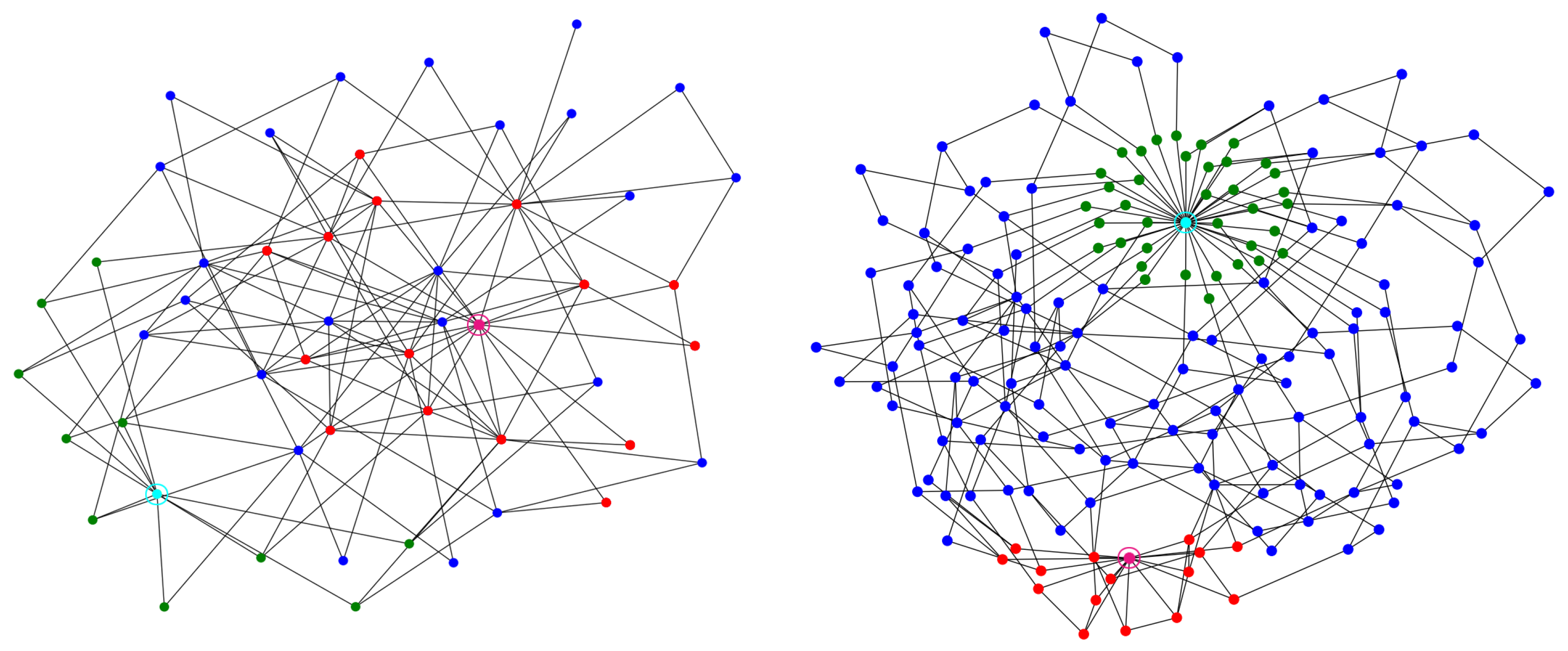
  In particular, we generate an extended BA undirected graph using the NetworkX Python module [36] (function extended_barabasi_albert_graph, input arguments $\mathtt{n}=50,\mathtt{m}=2,\mathtt{p}=0.15$, and $\mathtt{q}=0.35$); then, we denote t (the sink of the network) as the node with the highest betweenness centrality [37] and we add a new node s (the source of the network) connected to the 10 nodes with smallest closeness centrality [38,39]. With these operations, we obtain a graph $G_{\mathrm{BA}}$ of 51 nodes and $n=\left|E\right|=126$ edges, where the source s is connected to the 10 nodes and the sink t is connected to the $m=15$ nodes (see Figure 3-left).
  In the end, since, in real-world applications, truncated normal distributions seem to be very common (see Remark 7), in order to simulate a rather general maximum-flow regression problem, we chose a truncated normal distribution between 0 and 10, with a mean of 0, and a standard deviation of $5/3$, as a probability distribution p for the edge capacities (see Section 3.1.1); i.e.,

  $$c_i\sim p\equiv {\mathcal{N}}_{[0,10]}(5,5/3),\forall i=1,\dots ,n.$$

  (20)
• ${\mathcal{G}}_2=(G_{\mathrm{ER}},s,t,p)$. The graph $G_{\mathrm{ER}}$ of ${\mathcal{G}}_2$ characterizes a flow network built on an Erdos-Rényi (ER) model graph [40,41]. Put simply, an ER model graph is a random graph generated with a fixed number of nodes, where the edge $e_{ij}=(v_i,v_j)$ has a fixed probability of being created. This family of graphs is typically used to prove and/or find new properties that hold for almost all the graphs; for this reason, we consider a stochastic flow network based on an ER graph in our experiments.
  In particular, we generate an ER undirected graph using the NetworkX Python module [36] (function fast_gnp_random_graph, input arguments $\mathtt{n}=200,\mathtt{p}=0.01$) and we select its largest connected component $G_0$ (in terms of the number of vertices). Then, we add to $G_0$ two new nodes: a node s (the source of the network) connected to all the nodes with degree equal to 1, and a node t (the sink of the network) connected to the 15 most distant nodes from s. With these operations, we obtain a graph $G_{\mathrm{ER}}$ of 171 nodes and $n=\left|E\right|=269$ edges, where the source s is connected to 37 nodes and the sink t is connected to $m=15$ nodes (see Figure 3-right).
  In the end, we chose the truncated normal distribution (20) as the probability distribution p for the edge capacities.

Remark 7

(Regarding the truncated normal distribution for capacities). In a network describing a system of highroads, the capacity of a road is defined as $c=k\ell /S$ [42], where $k\in {\mathbb{R}}^{+}$ is a value depending on the type of the road, ℓ is the road length, and S is the average distance between two vehicles, typically chosen as a constant value. Then, assuming a network with all roads of the same type (i.e., k constant) and a truncated normal distribution for the length ℓ of the roads, the capacity can be modeled as a random variable with a truncated normal distribution. Therefore, generalizing the concept of the highroad capacity to other similar problems (e.g., a network of pipes, a communication network, etc.) the distribution (20) can be considered sufficiently generic for the numerical experiments of this section.

Given the stochastic flow networks ${\mathcal{G}}_1$ and ${\mathcal{G}}_2$, the corresponding maximum-flow regression problems consist of the approximation of the functions ${\mathit{F}}_1:{\mathbb{R}}^n\to {\mathbb{R}}^m$, $n=126$, $m=15$, and ${\mathit{F}}_2:{\mathbb{R}}^n\to {\mathbb{R}}^m$, $n=269$, $m=15$, respectively, where ${\mathit{F}}_1$ and ${\mathit{F}}_2$ are defined as in (16). For each $i=1,2$, we build the dataset ${\mathcal{D}}_i$ of ${\mathcal{G}}_i$ made of 10,000 pairs $(\mathit{c},\mathbf{\phi }={\mathit{F}}_i\left(\mathit{c}\right))\in {\mathbb{R}}^n\times {\mathbb{R}}^m$, where 3000 of them are used as the test set (${\mathcal{P}}_i$) and the remaining 7000 pairs are used to generate the multi-set ${\Theta }_i$ sampling $\vartheta \in \{1,\dots ,7000\}$ pairs. In particular, $80\%$ of the pairs in ${\Theta }_i$ are used as the training set (${\mathcal{T}}_i$) and the remaining $20\%$ are used as the validation set (${\mathcal{V}}_i$). An important aspect of our numerical experiments consists of analyzing the performance of the trained NNs, varying the quantity of available data for the training process (i.e., $\vartheta$), and not only varying the hyper-parameters related to the architecture and optimization method; in particular, we study the NN performances when the number of training and validation data is $\vartheta =7000,1000,500$. Indeed, in real-world problems, the amount of available data can be limited for many reasons (e.g., limited computational resources for simulations, limited time for measurements, etc.). Then, studying the performances of a regression model while decreasing $\vartheta$ is important to understand the sample efficiency of the model.

The fluxes ${\mathit{F}}_i\left(\mathit{c}\right)=\mathbf{\phi }$ for the dataset creation are computed using the maximum_flow NetworkX function that, specifically, allows the computatio of the flows for all the edges of the network (given the capacities $\mathit{c}$). Then, considering all the 10,000 simulations executed to build the dataset ${\mathcal{D}}_i$, and denoting ${\ell }_{max}^{\left(i\right)}\left(\mathit{c}\right)$ the length of the longest source-sink path in ${\mathcal{G}}_i\left(\mathit{c}\right)$, we observe that:

• ${\ell }_{min}\left({\mathcal{G}}_1\right)=4$, ${\ell }_{\mathrm{av}}\left({\mathcal{G}}_1\right)\approx 5.5$, and ${\ell }_{max}\left({\mathcal{G}}_1\right)=9$;
• ${\ell }_{min}\left({\mathcal{G}}_2\right)=7$, ${\ell }_{\mathrm{av}}\left({\mathcal{G}}_2\right)\approx 10.7$, and ${\ell }_{max}\left({\mathcal{G}}_2\right)=17$;

where ${\ell }_{min}\left({\mathcal{G}}_i\right),{\ell }_{\mathrm{av}}\left({\mathcal{G}}_i\right)$, and ${\ell }_{max}\left({\mathcal{G}}_i\right)$ are the minimum, the average, and the maximum lengths, respectively, of the longest source-sink path of the flow for ${\mathcal{G}}_i$ with respect to ${\mathcal{D}}_i$, i.e.,

$${\ell }_{min}\left({\mathcal{G}}_i\right):=\underset{(\mathit{c},\phi )\in {\mathcal{D}}_i}{min}{\ell }_{max}^{\left(i\right)}\left(\mathit{c}\right),$$

(21)

$${\ell }_{\mathrm{av}}\left({\mathcal{G}}_i\right):=\frac{1}{|{\mathcal{D}}_i|}\sum _{(\mathit{c},\phi )\in {\mathcal{D}}_i}{\ell }_{max}^{\left(i\right)}\left(\mathit{c}\right),$$

(22)

and

$${\ell }_{max}\left({\mathcal{G}}_i\right):=\underset{(\mathit{c},\phi )\in {\mathcal{D}}_i}{max}{\ell }_{max}^{\left(i\right)}\left(\mathit{c}\right).$$

(23)

The values reported in items 1 and 2 show that, on the average, in a radius of the length ${\ell }_{\mathrm{av}}\left({\mathcal{G}}_i\right)$ from the sink t, it is likely to find almost all the nodes characterizing the maximum-flow of the network ${\mathcal{G}}_i$. This information is then taken into account while choosing the depth values for the construction of the GINNs in the following Section 3.3.1. Indeed, we recall that the number of consecutive GI layers in an NN tells us if the input feature of node $v_i$ contributes to the computation of the output feature of node $v_j$ (see Proposition 1). Therefore, it is interesting to verify if the regression performance of a GINN improves or not, when the number of GI layers is related to one of the quantities (21)–(23).

3.3.1. NN Architectures, Hyper-Parameters, and Training

In the numerical experiments of this section, we study and compare the performances of MLPs and GINNs concerning the maximum-flow regression problems related to ${\mathit{F}}_1$ and ${\mathit{F}}_2$. Then, we consider the two archetypes of NN architectures: an MLP archetype and a GINN archetype.

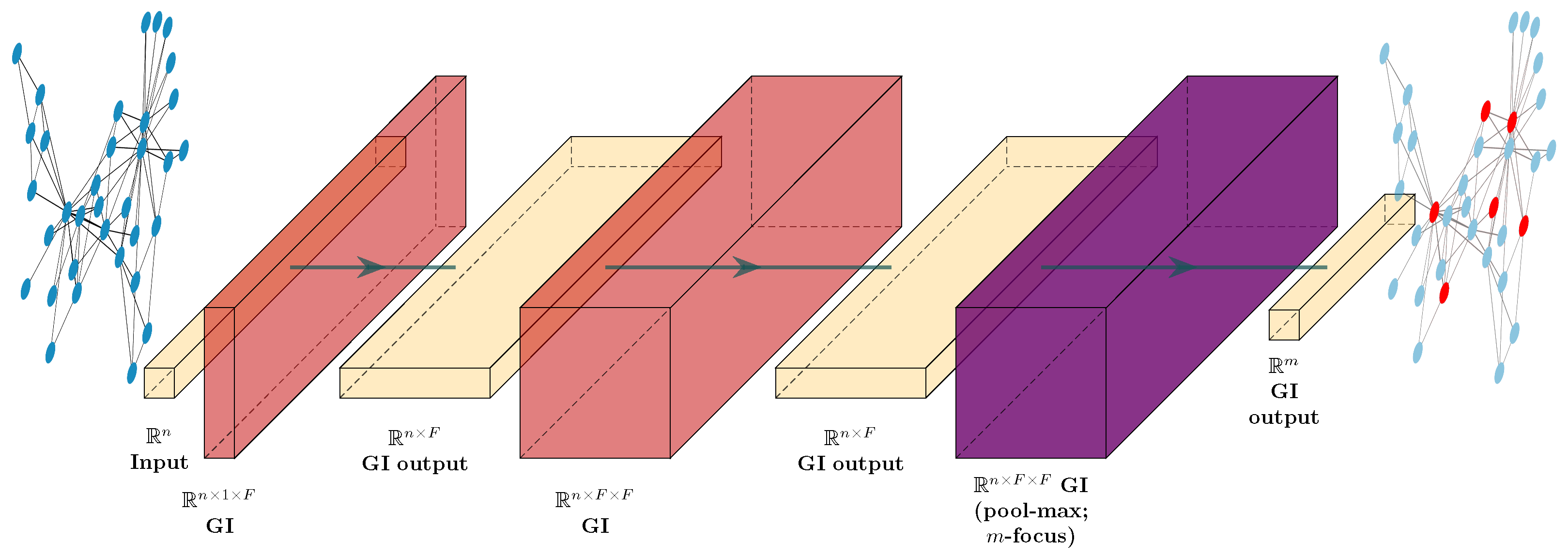
• MLP Archetype: The NN architecture is characterized by one input layer $L_0$, $H\in \mathbb{N}$, hidden layers $L_1,\dots ,L_H$ with a nonlinear activation function f, and one output layer $L_{H+1}$ with a linear activation function. The output layer is characterized by m units, while all the other layers are characterized by n units. Finally, we apply a batch normalization [43] before the activation function for each hidden layer $L_1,\dots ,L_H$. See Figure 4.
• GINN Archetype: The NN architecture is characterized by one input layer $L_0$ of n units, $H\in \mathbb{N}$ hidden GI layers $L_1^{GI},\dots ,L_H^{GI}$ with a nonlinear activation function f, and one output layer $L_{H+1}^{GI}$ with a linear activation function. All the GI layers are built with respect to the adjacency matrix $A_L\in {\mathbb{R}}^{n\times n}$ of the line graph of the network (see Section 3.2.1) and they are characterized by $F\in \mathbb{N}$ filters (i.e., output features). Then, the number of input features K of the GI layer $L_h^{GI}$ is $K=F$, if $h>1$, and $K=1$, if $h=1$. As for the MLP archetype, we apply a batch normalization before the activation function of each hidden layer. Finally, the output layer is characterized by a pooling operation and by the application of a mask (see Section 2.3) to focus on the m units corresponding to the m target flows. See Figure 5.

For our experiments, given the two NN archetypes above, we built a set of untrained NN models, varying the main hyper-parameters of the architectures. In particular, for the MLPs, we varied the hyper-parameters H and f (i.e., the depth and activation functions of the hidden layers), while for the GINNs, we also varied F (i.e., the number of filters of the GI layers) and the pooling operation. Specifically, the hyper-parameters vary among these values:

• MLP archetype.$f\in \left\{\mathrm{relu},\mathrm{elu},\mathrm{swish},\mathrm{softplus}\right\}$ and $H\in \{2,3,4,5\}$. We do not use deeper MLPs to avoid the so-called degradation problem [44], i.e., the problem in which increasing the number of hidden layers causes the performance of an NN to saturate and degrade rapidly.
• GINN archetype.$f\in \left\{\mathrm{relu},\mathrm{elu},\mathrm{swish},\mathrm{softplus}\right\}$, $F\in \{1,5,10\}$, and pooling operations in $\{max,\mathrm{mean}\}$ (only if $F=5,10$); $H\in \{3,5,7,9\}$ for ${\mathcal{G}}_1$ and $H\in \{4,9,14,19\}$ for ${\mathcal{G}}_2$. In particular, we select these values of H because they are a discrete interval around the value ${\ell }_{\mathrm{av}}\left({\mathcal{G}}_i\right)$, also including cases near, or equal to, the minimum and maximum values ${\ell }_{min}\left({\mathcal{G}}_i\right)$ and ${\ell }_{max}\left({\mathcal{G}}_i\right)$, respectively.

Then, these models are all trained on $\vartheta =7000,1000,500$ input–output pairs sampled from ${\mathcal{D}}_i-{\mathcal{P}}_i$, using a mini-batch size $\beta =128,64,32$; the weight initialization is a Glorot normal distribution [45] for the MLPs and it varies among a Glorot normal and a normal distribution $\mathcal{N}(0,0.5)$ for the GINNs. All the biases are initialized as zeroes.

The remaining training options are fixed and shared by all the models during the training. In particular, these options are:

• Mean square error (MSE) loss, i.e.,

  $$\mathrm{loss}\left(\mathcal{B}\right):=\frac{1}{m}\sum _{j=1}^m\left(\frac{1}{\left|\mathcal{B}\right|}\sum _{(\mathit{c},\phi )\in \mathcal{B}}{({\widehat{\phi }}_j-{\phi }_j)}^2\right),$$

  (24)

  where $\mathcal{B}$ is any generic batch of input–output pairs;
• The Adam optimizer [46] (learning rate $ϵ=0.002$, moment decay rates ${\rho }_1=0.9$, ${\rho }_2=0.999$);
• Early stopping regularization [20,47] (200 epochs of patience, restore best-weights), to avoid overfitting;
• Learning rate reduction on plateau [47] (reduction factor $\alpha =0.5$, 100 epochs of patience, minimum learning rate $ϵ={10}^{-6}$).

The training of all the NN models, with respect to all the different training configurations, returns 3168 trained NNs; in particular, we have 144 MLPs and 1140 GINNs, for each stochastic flow network ${\mathcal{G}}_1$ and ${\mathcal{G}}_2$.

3.3.2. Performance Analysis of Maximum-Flow Regression

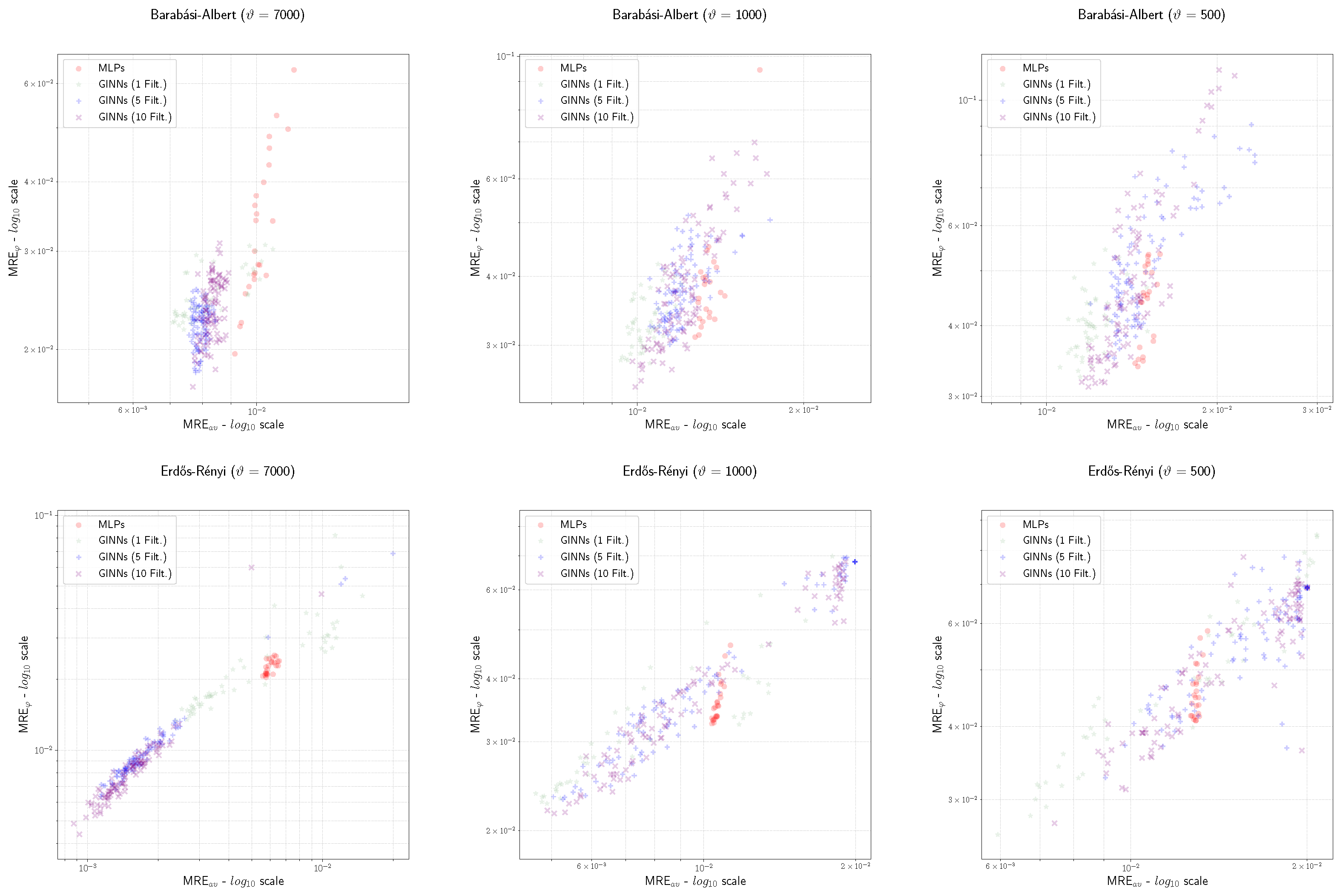
To evaluate the performance of an NN trained with respect to the maximum-flow regression task, we consider the errors MRE${}_{av}$ and MRE${}_{\phi }$ (see Section 3.2 and Equations (18) and (19), respectively) measured on the test set. In particular, to better analyze the performances, we visualize the NNs as points in the $({\mathrm{MRE}}_{av},{\mathrm{MRE}}_{\phi })$ plane (see Figure 6 and Figure 7). Then, the nearer a point is to the origin (i.e., the ideal zero-error NN), the better the regression performances of the corresponding NNs are. We decide to use this representation because of the characteristics of the errors reported in Remark 6. Indeed, it is important to analyze the behavior of the NNs with respect to MRE${}_{av}$ and MRE${}_{\phi }$ together.

We start the analysis with the first stochastic flow network ${\mathcal{G}}_1$. In general, looking at Figure 6, we clearly see that the GINNs have better regression performances than the MLPs. In particular:

(1)

The MRE${}_{\phi }$ of the GINNs is generally smaller than the MLPs, and this effect increases with $\vartheta$;

(2)

The MRE${}_{av}$ of the GINNs is almost always smaller than the MLPs, and this effect seems to be almost stable while varying $\vartheta$;

(3)

Looking at the hyper-parameter F, we observe that the cases with $F=1,10$ generally perform better with fewer training samples (i.e., $\vartheta =1000,500$) while the cases with $F=5$ generally perform better with $\vartheta =7000$. This phenomenon suggests that increasing the number of filters can improve the quality of the training, even if a clear rule for the best choice of F is not apparent.

We continue the analysis with the second stochastic flow network ${\mathcal{G}}_2$, increasing the size and complexity of the flow network. Indeed, the graph $G_{\mathrm{BA}}$ of ${\mathcal{G}}_1$ is characterized by a reduced complexity of the maximum-flow problem, because the BA graphs are generated using a preferential attachment criterion that keeps the average length of the maximum source-sink path ${\ell }_{\mathrm{av}}\left({\mathcal{G}}_1\right)$ small, even when increasing the nodes of the graph (this phenomenon was observed during some preliminary experiments).

Looking at Figure 7, we notice the same characteristics observed for ${\mathcal{G}}_1$, but much more emphasized. In particular, for each $\vartheta =7000,1000,500$, we clearly see that the GINNs generally outperform the MLPs, especially with respect to the MRE${}_{av}$. The reason for these similarities probably lies in the nature of the graphs $G_{\mathrm{BA}}$ and $G_{\mathrm{ER}}$ of ${\mathcal{G}}_1$ and ${\mathcal{G}}_2$, respectively; indeed, the ER graphs are used to represent generic graphs and are typically used to show properties that hold for almost all the graphs. On the other hand, the graph $G_{\mathrm{BA}}$ is simpler than $G_{\mathrm{ER}}$. Then, it is reasonable that the observations made for ${\mathcal{G}}_1$ are confirmed looking at ${\mathcal{G}}_2$ and it is reasonable that the performance differences observed in ${\mathcal{G}}_2$ are less emphasized in ${\mathcal{G}}_1$, since the maximum-flow problem on $G_{\mathrm{BA}}$ is less complex than on $G_{\mathrm{ER}}$.

Remark 8

(GINNs, small MRE${}_{av}$, and regressions on graphs). We have just observed that the GINNs genrally perform better than MLPs for regression tasks on graphs but, if we focus on the MRE${}_{av}$ values, the GINNs clearly show better performances (see Figure 6 and Figure 7 and

Table 1. Network ${\mathcal{G}}_1$. Top three GINNs and MLPs, for $\vartheta =7000,1000,500$. Models are sorted with respect to the MRE${}_{av}$ error; the “rank” column describes their global position with respect to all the other models.

${\mathcal{G}}_1$	GINNs								MLPs
$\mathbf{\vartheta }$	Rank	MRE${}_{\mathit{av}}$	$\mathbf{H}$	$\mathit{F}$	$\mathit{f}$	$\mathbf{\beta }$	Pool.	Init.	Rank	MRE${}_{\mathit{av}}$	$\mathbf{H}$	$\mathit{f}$	$\mathbf{\beta }$
7000	1/528	0.00707	9	1	elu	64	-	G.Norm.	446/528	0.00914	3	swish	32
	2/528	0.00712	9	1	elu	128	-	Norm.	453/528	0.00934	3	swish	64
	3/528	0.00713	9	1	elu	32	-	Norm	455/528	0.00939	4	swish	32
1000	1/528	0.00933	9	1	softplus	32	-	G.Norm.	338/528	0.01272	5	softplus	32
	2/528	0.00940	7	1	elu	32	-	Norm.	353/528	0.01289	4	elu	32
	3/528	0.00952	7	1	elu	32	-	G.Norm.	357/528	0.01292	5	elu	32
500	1/528	0.01056	7	1	softplus	32	-	Norm.	263/528	0.01433	5	softplus	32
	2/528	0.01077	5	1	relu	32	-	G.Norm.	279/528	0.01448	5	softplus	64
	3/528	0.01092	7	1	softplus	32	-	G.Norm.	284/528	0.01452	4	softplus	32

and

Table 2. Network ${\mathcal{G}}_2$. Top three GINNs and MLPs, for $\vartheta =7000,1000,500$. Models are sorted with respect to the MRE${}_{av}$ error; the “rank” column describes their global position with respect to all the other models.

${\mathcal{G}}_1$	GINNs								MLPs
$\mathbf{\vartheta }$	Rank	MRE${}_{\mathit{av}}$	$\mathbf{H}$	$\mathit{F}$	$\mathit{f}$	$\mathbf{\beta }$	Pool.	Init.	Rank	MRE${}_{\mathit{av}}$	$\mathbf{H}$	$\mathit{f}$	$\mathbf{\beta }$
7000	1/528	0.00087	14	10	softplus	32	max	G.Norm.	442/528	0.00557	2	elu	32
	2/528	0.00092	14	10	softplus	32	mean	G.Norm.	445/528	0.00571	5	softplus	64
	3/528	0.00099	12	10	softplus	32	mean	G.Norm	446/528	0.00573	5	elu	32
1000	1/528	0.00465	9	1	elu	32	-	G.Norm.	263/528	0.01038	3	softplus	32
	2/528	0.00478	19	1	elu	32	-	G.Norm.	264/528	0.01038	2	swish	32
	3/528	0.00479	14	1	softplus	32	-	Norm.	267/528	0.01043	3	softplus	64
500	1/528	0.00593	14	1	elu	32	-	G.Norm.	114/528	0.01266	2	swish	32
	2/528	0.00674	14	1	softplus	32	-	G.Norm.	118/528	0.01272	2	swish	64
	3/528	0.00688	19	1	softplus	32	-	G.Norm.	119/528	0.01272	5	softplus	32

). Specifically, Table 1 and Table 2 show the three GINNs and MLPs with lowest MRE${}_{av}$ value on the test sets of ${\mathcal{G}}_1$ and ${\mathcal{G}}_2$, respectively. The better performances of the GINNs, with respect to this error measure, are particularly important if we extend the regression problem, e.g., if we want to learn all the flow values ${\phi }^{\ast \left(\mathit{c}\right)}\left(e_1\right),\dots ,{\phi }^{\ast \left(\mathit{c}\right)}\left(e_n\right)$ on the edges of the graph and not only the ones characterizing the maximum-flow φ reaching the sink. Indeed, in this case, an NN with small errors on the single elements of the target vector is fundamental, while an NN with small errors on the sum of the elements of the target vector is useless; for this reason, in vector-valued regression tasks, we use loss functions such as (24) (evidently similar to the performance measure MRE${}_{av}$). In conclusion, we believe that the GINNs have great potential in the field of regression graphs.

We continue to conclude the performance analysis, and we analyze how the errors of the NN models change when varying the hyper-parameters.

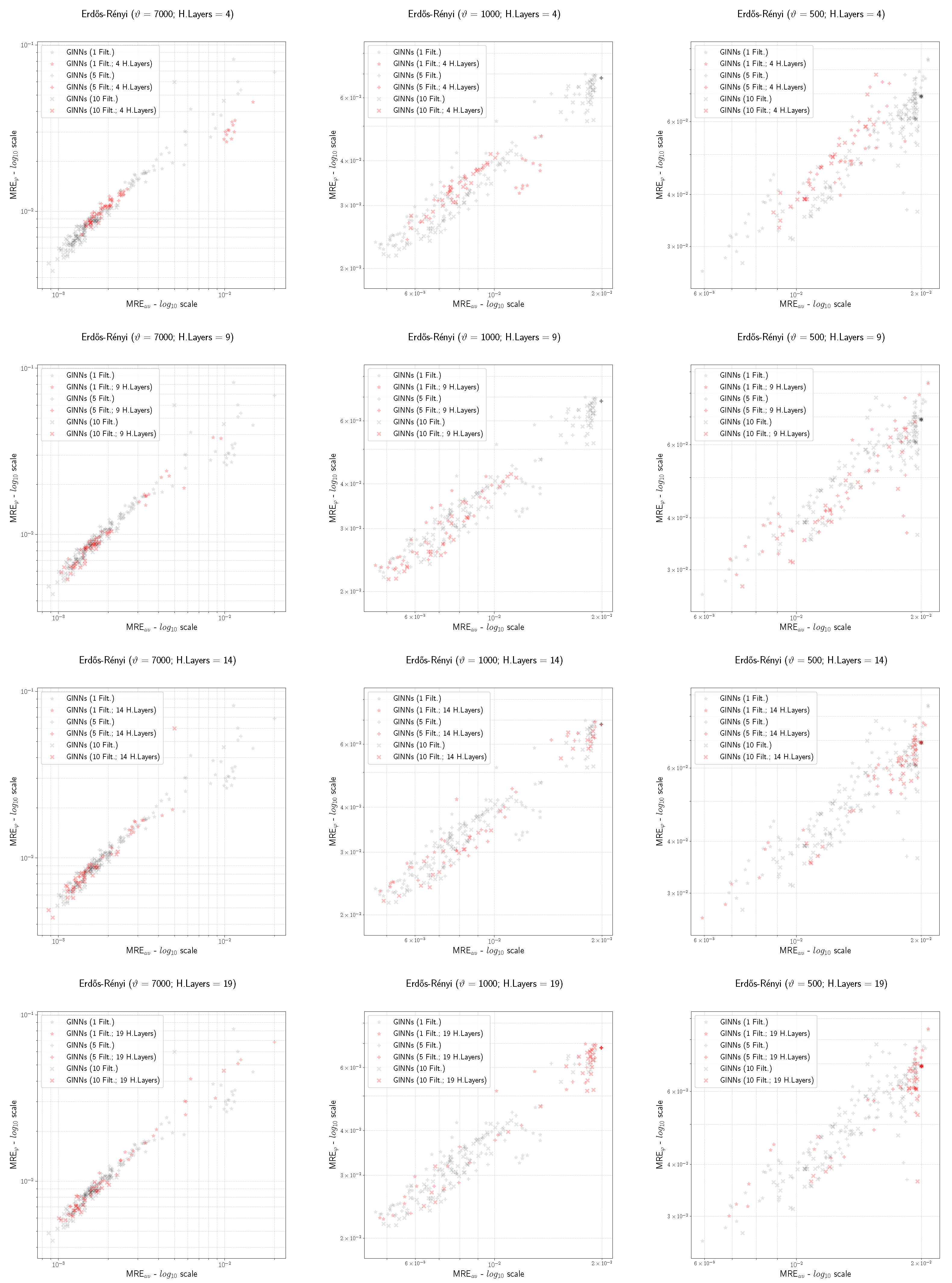
The first observation is related to the activation functions and the mini-batch size. We observe that the trained NN models (both GINNs and MLPs) generally exhibit worse regression performances with a relu activation function and a mini-batch size equal to 128; in Figure 8, we report the same scatterplots of Figure 6 and Figure 7 but without the points corresponding to the NNs with the relu activation function or a mini-batch size equal to 128. It is worth noting that the general observations concerning the NN performances are even more evident when removing these models. Moreover, among the remaining models, we do not observe activation functions or mini-batch size values that are evidently better than the others; in general, as can be expected, we only observe a few advantages of using a mini-batch size of 32 samples instead of a mini-batch size of 64 samples, while decreasing $\vartheta$.

From now on, we do not include in our analyses the models characterized by a relu activation function or mini-batch size equal to 128. Moreover, we only focus on the GINN models and, in particular, on their performances with respect to the hyper-parameter H, characterizing the number of hidden layers. Indeed, the remaining hyper-parameters (pooling operations and weight initializations) do not seem to have a particular impact on the results.

The study of the GINN performances with respect to H is particularly interesting if we consider Proposition 1. In fact, from this proposition, we expect the GINN models to have a better performance if the depth H is such that $H+1\gtrsim {\ell }_{\mathrm{av}}\left({\mathcal{G}}_i\right)$. This guess is indeed satisfied. In particular, for ${\mathcal{G}}_1$, we see that by increasing the depth H, we obtain GINNs with better performances in general (see Figure 9). On the other hand, for ${\mathcal{G}}_2$ we observe a slightly different behavior. The GINNs that are sufficiently deep (i.e., $H\ge 9$) show better performances than the GINNs with $H=4$, but their errors tend to increase with a small $\vartheta$; in particular, the more H is greater than ${\ell }_{\mathrm{av}}\left({\mathcal{G}}_2\right)$, the more the GINN performances seem to deteriorate (see Figure 10). To summarize, the depth in a GINN model is very important to obtaining good regression abilities, keeping in mind Proposition 1. Nonetheless, the practice of using as much of a GI layer as possible is not always the best choice, and this topic deserves attention in future work.

Remark 9

(Training time). Along the conducted experiments (with training that occurred more than 3000 times), we find that the average training time for the GINN models is approximately 20 min in total, and one second per epoch; on the other hand, the average training time for the MLP models is approximately 10 min in total and half a second per epoch. Nonetheless, we point out that the difference in training times between GINNs and MLPs can be reduced with code optimization. Indeed, the GINN layers are a custom class of TensorFlow NN layers developed on purpose by the authors for numerical experiments. The code of TensorFlow’s FC layers is extremely optimized. Therefore, at the present time, the GINNs and MLPs cannot be compared in terms of computational costs. More details about the average training times per epoch of the models are reported in

Table 3. Global statistics of the average training time per epoch for GINN and MLP models, expressed in seconds.

	Avg. Time per Epoch (s)
	GINNs	MLPs
Mean	1.099	0.565
Std	1.359	0.292
25th perc.	0.318	0.380
50th perc.	0.567	0.431
75th perc.	1.296	0.632

, and this quantity is indicative of the training computational cost of the NNs. However, we recall that the experiments take into account more than three thousand models, each one with a different training configuration that characterizes the training time per epoch. All the training was performed on a workstation with a CPU of 4 Core and 8 Threads, 32 GB of RAM, and a GPU Nvidia 1080 8 GB.

3.4. GINNs for Flux Regression in Discrete Fracture Networks

In Section 3.3, we showed the regression abilities and the potentialities of the GINN models for the maximum-flow regression problem, i.e., for a problem representative of generic real-world applications.

In this section, we address a specific real-world application where GINNs can be useful; in particular, we consider an uncertainty quantification (UQ) problem related to underground flows in fractured media. Flow characterization in underground fractured media is an interesting problem for many applications, such as civil engineering, industrial engineering, and environmental analyses. A helpful model to describe the flow in an underground network of fractures is represented by the discrete fracture network (DFN) models [48,49,50]. These models express the fractures as two-dimensional polygons into a three-dimensional domain, and each fracture is described by specific hydro-geological properties (e.g., fracture transmissivity) and geometrical properties (e.g., barycenter position and orientation). Intersections between fractures, denominated “traces”, define flux exchange phenomenons, such that the flow model is typically ruled by the following assumptions: (i) the rock matrix is impenetrable; (ii) the Darcy law is used for the flux propagation on each fracture; and (iii) the head continuity and flux balance is imposed on all the traces. However, since the hydro-geological and geometrical characteristics of the network of fractures are usually not accessible in detail, the DFN models are typically generated by sampling their hydro-geological and geometrical features from known distributions [51,52,53,54]. Therefore, a statistical approach is required to study real fractured media, resorting to UQ analyses.

In recent literature, several new methods have been proposed to reduce the computational costs of the DFN flow simulations (e.g., see [55,56,57]); nonetheless, they are still computationally expensive in many situations and the UQ analyses can involve thousands of these simulations. Therefore, it is fundamental to take into account the techniques for the complexity reduction, such as machine learning-based techniques (e.g., see [16,17,58]). In particular, in [16,17], NN models are trained on datasets built using DFN simulations to provide surrogate models; finally, in a negligible amount of time, the NN models are used to generate a large set of approximated DFN flow simulation results, which are particularly useful to speed up the UQ analyses.

In this section, the idea is to take advantage of the DFN’s graph structure to build GINN models and to analyze the advantages of using such models for the DFN flux regression tasks instead of the more classic NN architectures (e.g., MLPs or multi-task NNs).

3.4.1. The DFN Model and the Flux-Regression Task in DFNs

Here, for the reader’s convenience, we briefly describe the problem of the flow simulations in DFNs. We point the interested reader to [55,56,57] for full details.

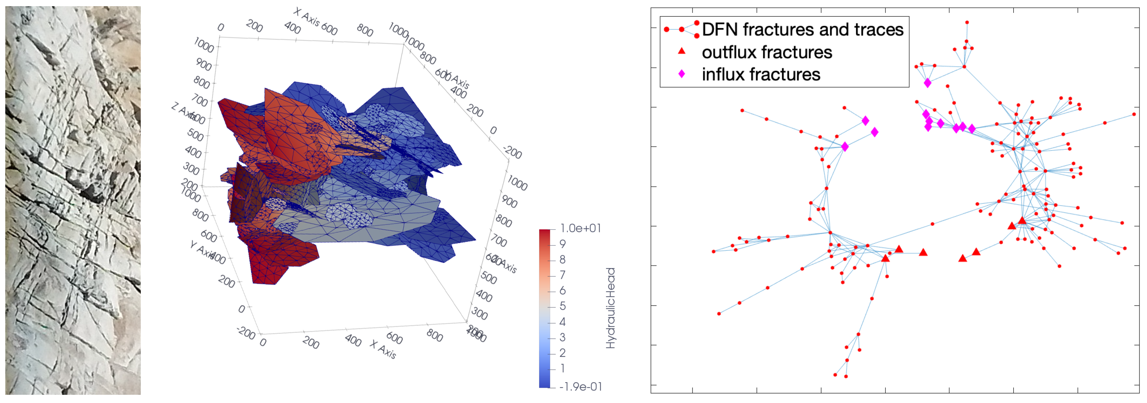
A DFN model is a discrete representation of an underground network of fractures in a fractured rock medium using a set of intersecting planar polygons (the fractures) in a three-dimensional domain $\mathbb{D}\subset {\mathbb{R}}^3$ (the rock medium); see Figure 11 for a DFN example. Each fracture (i.e., polygon) is labeled and identified by an index belonging to an arbitrary set I; i.e., for each $i\in I$, we denote each fracture by ${\mathcal{F}}_i$. Then, a DFN is defined as the union of all the fractures, i.e., ${\cup }_{i\in I}{\mathcal{F}}_i$. Since the traces, i.e., the segments obtained from the intersection of two or more fractures that connect the fractures define a network, a DFN can be represented as a graph where the fractures are the nodes and the traces are edges (see Figure 11).

Each fracture in a DFN is characterized by a transmissivity parameter ${\kappa }_i$ and by geometrical properties, such as the size and the orientation in ${\mathbb{R}}^3$. These characteristics are generally sampled from known probability distributions, and they characterize the flow simulations of the DFN. Indeed, a DFN flow simulation depends both on the geometry and the hydro-geological properties of the fractures, such as the transmissivities ${\kappa }_i$ of the fractures.

The DFN flux regression problem addressed in this section is characterized as follows. The DFN considered consists of $n=158$ fractures and we donote it by DFN158. The geometry of DFN158 is fixed, and the fractures are immersed into a domain $\mathbb{D}$ described by a cube of 1000 m along the long edge (see Figure 11). The domain boundary conditions are such that a fixed pressure difference $\Delta \mathrm{H}=10$ m is imposed between two opposite faces of $\mathbb{D}$, therefore representing an inlet and outlet face, respectively. Moreover, those fractures cut by the inlet and outlet faces of the domain are defined as inflow and outflow fractures, respectively. The edges of all the other fractures are insulated (homogeneous Neumann condition). It is possible to observe that the fixed geometry and the given boundary conditions affect the flux directionality in DFN158; on the other hand, the fracture transmissivities characterize the flow intensity exiting from the outflow fractures. In particular, we assume that the fracture transmissivities of the fractures ${\mathcal{F}}_1,\dots ,{\mathcal{F}}_n$ are isotropic parameters ${\kappa }_1,\dots ,{\kappa }_n$, respectively, described by random variables with a log-normal distribution [51,52]:

$${log}_{10}{\kappa }_i\sim \mathcal{N}(-5,1/3),\forall i=1,\dots ,n.$$

In the test case considered, we use octagons to represent the fractures and they have been randomly created according to the distributions in [53,54]. For their geometrical properties: a truncated power law distribution for the fracuture radii, with an exponent $\gamma =2.5$ and an upper and lower cut-off $r_u=560$ and $r_0=50$, respectively; a Fischer distribution for fracture orientations, with a mean direction $\mu =(0.0065,-0.0162,0.9998)$ and a dispersion parameter of $17.8$; and a uniform distribution for the mass centers of the fractures. However, the first eight fractures ${\mathcal{F}}_1,\dots ,{\mathcal{F}}_8$ are not randomly sampled but are created to ensure an inlet-outlet path for the flow, where ${\mathcal{F}}_1$ is an inflow fracture and ${\mathcal{F}}_8$ is an outflow fracture.

Together with the boundary conditions described above, the geometry of DFN158 is such that we have $m=7$ outflow fractures in DFN158. Therefore, we can define a flux function representing the DFN flow simulations for DFN158; i.e., a function $\mathit{F}:{\mathbb{R}}^n\to {\mathbb{R}}^m$ such that, for each vector $\kappa ={[{\kappa }_1,\dots ,{\kappa }_n]}^{\top }\in {\mathbb{R}}^n$ of fracture transmissivities with $n=158$, it returns the vector $\mathit{F}\left(\mathbf{\kappa }\right)=\mathbf{\phi }={[{\phi }_1,\dots ,{\phi }_m]}^{\top }\in {\mathbb{R}}^m$ of fluxes exiting from the m outflow fractures, $m=7$.

Now, assuming the need to perform UQ analyses of the fluxes ${\phi }_1,\dots ,{\phi }_m$ of DFN158 while varying the fracture transmissivities, it is worth considering the flux regression problem that looks for NN-based approximations $\widehat{\mathit{F}}$ of $\mathit{F}$.

3.4.2. Performance Analysis of DFN Flux Regression

In this subsection, we extend the numerical experiments and analyses of Section 3.3 to the example represented by DFN158. Then, we study and compare the performances of the MLPs and GINNs concerning the flux regression problem related to the function $\mathit{F}:{\mathbb{R}}^n\to {\mathbb{R}}^m$ described in Section 3.4.1. The two archetypes of MLP and GINN architectures are the same as in Section 3.3.1, as are most of the hyper-parameter values and the training options used; the only differences are the following:

• $\vartheta =1000,500$ (number of training and validation data);
• $\beta =64,32$ (mini-batch size);
• The relu activation function is not considered in the experiments;
• For the GINN models, we consider the depth parameter values $H\in \{4,7,9,14,19\}$. The rationale behind this choice is that it is a set of values around 8, which is the number of deterministic fractures that, on average, represent an inlet-outlet flow path for DFN158 (in the absence of a value equivalent to ${\ell }_{\mathrm{av}}$ that cannot be easily computed for DFN158);
• The GI layers are built with respect to the adjacency matrix A of DFN158; indeed, we do not need to introduce the line graph of the network since the features (i.e., the transmissivities) are assigned to the nodes of the graph and not to the edges.

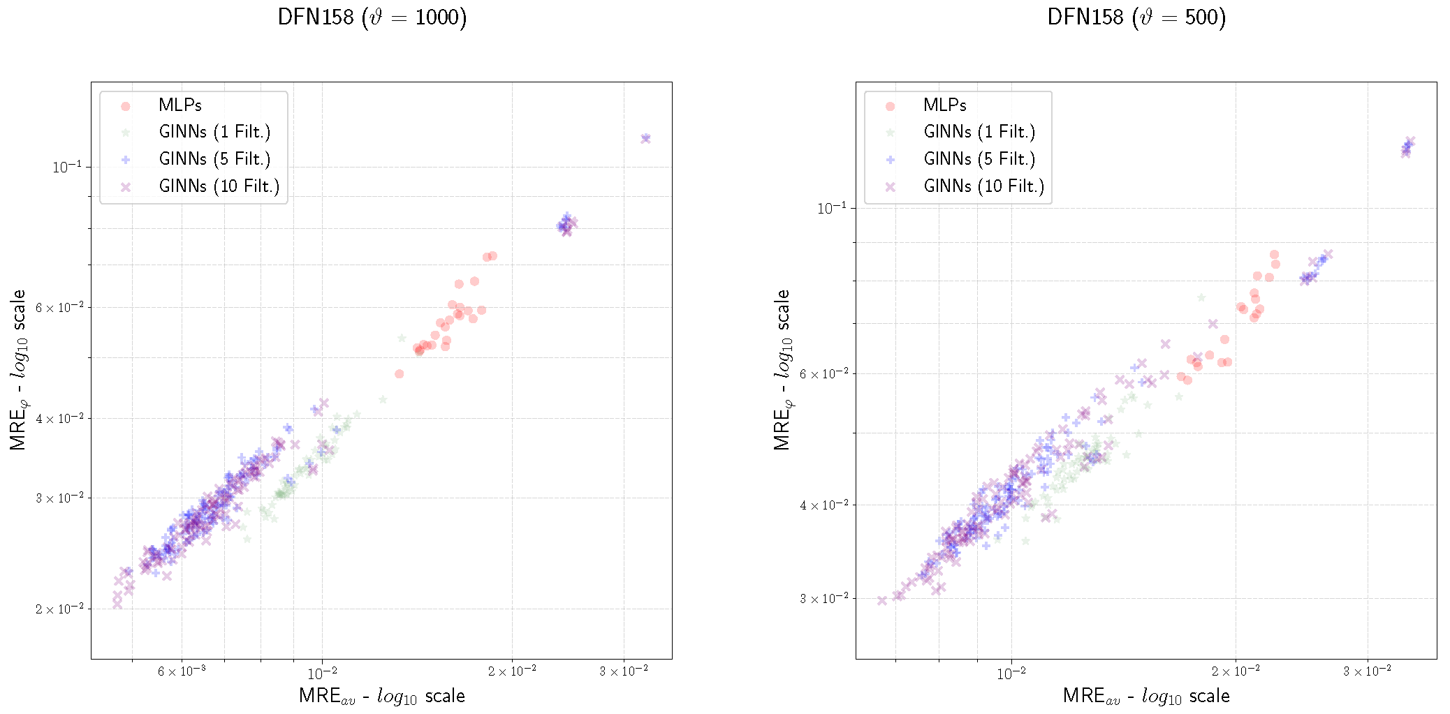
As in Section 3.3.2, we evaluate the performance of the NNs trained with respect to the DFN flux regression task measuring the errors MRE${}_{av}$ and MRE${}_{\phi }$ on the test set (also, in this case, $\mathcal{P}$ is made of 3000 samples). Then, we visualize the results of the NNs as points in the $({\mathrm{MRE}}_{av},{\mathrm{MRE}}_{\phi })$ plane (see Figure 12). Analyzing the error values and looking at the scatter plots of Figure 12, we clearly observe that the GINN models outperform the MLPs, and that they are characterized by more regular error behaviors than the GINNs trained for the maximum-flow regression task, with respect to the filter hyper-parameter (see Section 3.3.2). In particular:

• Both the MRE${}_{\phi }$ and the MRE${}_{av}$ of the GINNs are almost always smaller than the ones of the MLPs, independently of $\vartheta$;
• Looking at the filter hyper-parameter F, we observe that the GINN performances are better as F increases (from $F=1$, to $F=5$, to $F=10$).

We continue the analysis of studying the relationships between the GINN errors and the other hyper-parameters of the models. With respect to the activation functions, we observe that the GINN models with the elu activation functions have, in general, slightly better performances than other models; on the other hand, all the GINN models with the worst performances (i.e., the points in the top-right corners of Figure 12) have softplus activation functions. Concerning the mini-batch size $\beta$, we observe that the GINNs with the best performances (corresponding to points in the bottom-left corners of Figure 12) are trained with $\beta =32$. Similar results hold for the weights initialization, where the best performing GINNs are initialized with a Glorot normal distribution. Concerning the pooling operations, we do not observe particular differences in the error values of GINN models using a max-pooling or a mean-pooling operation.

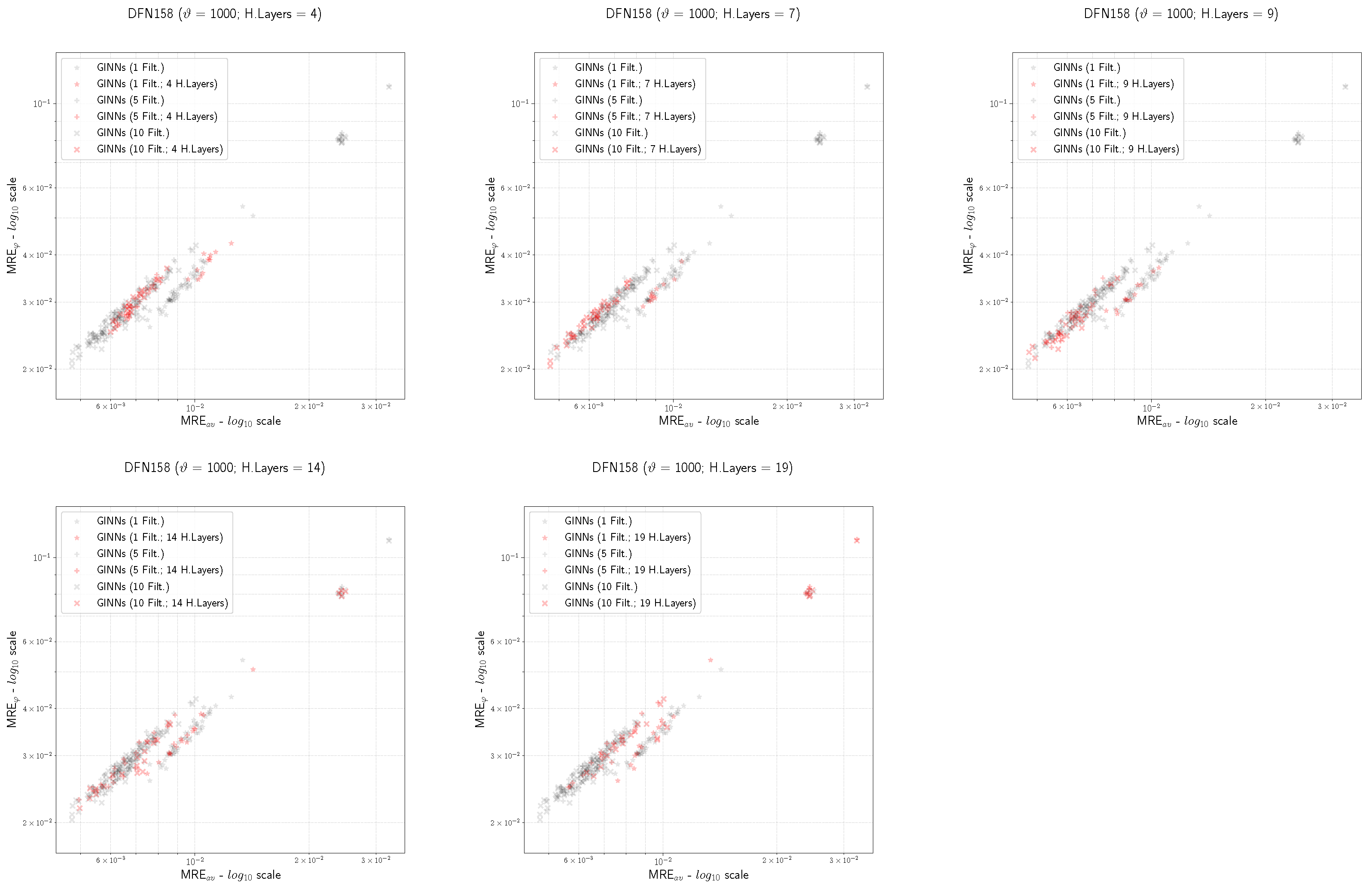
Analogous to Section 3.3.2, we conclude with a focus on the error behaviors with respect to the depth H of the GINN models. Moreover, for the DFN flux regression task, we observe that the depth H of the model can improve the regression quality. In particular, for each $\vartheta =1000,500$, we observe that the best performances are obtained by the GINNs with a depth of $H=7,9,14$, while both the shallowest and the deepest GINNs ($H=4,19$) have higher errors (see Figure 13 and Figure 14). In accordance with Proposition 1 and the observations of Section 3.3.2, this characteristic let us deduce that, on average, the maximum inlet-outlet flux path in DFN158 is probably made of 8 to 15 fractures; i.e., a value not so far from the length of the inlet-outlet path defined by the fractures ${\mathcal{F}}_1,\dots ,{\mathcal{F}}_8$.

4. Conclusions

In this work, we presented the graph-informed (GI) layers, a new type of spatial-based graph convolutional layer, designed for regression tasks on graph-structured data. With respect to the other types of GCN layers, our GI layers stand out for their tensor formulation (see (8)), managing multiple input/output features; moreover, these layers let users build deep NN architectures which are able to exploit the depth needed to improve the regression performances (see Proposition 1 and Section 3.3.2 and Section 3.4.2). The GI layers have been formally defined, from the simplest version to the most general and tensor version. Moreover, additional optional operations are introduced: the pooling operation and mask operations.

To study the regression abilities of graph-informed NNs (GINNs), i.e., NNs made from GI layers, we trained thousands of NN models (both GINNs and MLPs) on two maximum-flow regression problems, with networks based on a Barabási–Albert graph (${\mathcal{G}}_1$) and an Erdos–Rényi graph (${\mathcal{G}}_2$). We selected the maximum-flow regression problem as a representative test since it is a sufficiently general problem to demonstrate the applications in many topics of the network analysis. Analyzing the approximation errors of the NNs, we observed that the GINNs have better performances than the MLPs. in general. In particular, for ${\mathcal{G}}_2$, the GINNs in almost all the cases outperform the MLPs. The study of the regression performances also showed an interesting relationship between small errors and a depth greater than, or equal to, the average length of the maximum source-sink path in the stochastic network.

After the test on the maximum-flow regression task, we illustrated an example of a possible application of the GINNs to a real-world problem: a DFN flux regression problem, i.e., an uncertainty quantification problem for the characterization of the exiting flux distribution of an underground network of fractures. In this practical application, the GINN models completely outperform the MLPs; moreover, both the depth and the filter hyper-parameters of the GINNs proved to be significant enough to improve the approximation quality of the target function.

In conclusion, we believe that our work introduces a new, useful, contribution to the family of spatial-based graph convolutional networks; indeed, the numerical experiments illustrated here show that the new GI layers and the GINNs have great potentialities in the framework of regression tasks on graph-structured data.

References

1. Brandes, U.; Erlebach, T. (Eds.) Network Analysis—Methodological Foundations; Theoretical Computer Science and General Issues; Springer: Berlin/Heidelberg, Germay, 2005; Volume 3418. [Google Scholar] [CrossRef]
2. Gori, M.; Monfardini, G.; Scarselli, F. A new model for learning in graph domains. In Proceedings of the 2005 IEEE International Joint Conference on Neural Networks, Montreal, QC, Canada, 31 July–4 August 2005; Volume 2, pp. 729–734. [Google Scholar] [CrossRef]
3. Micheli, A. Neural Network for Graphs: A Contextual Constructive Approach. IEEE Trans. Neural Netw. 2009, 20, 498–511. [Google Scholar] [CrossRef]
4. Scarselli, F.; Gori, M.; Tsoi, A.C.; Hagenbuchner, M.; Monfardini, G. The Graph Neural Network Model. IEEE Trans. Neural Netw. 2009, 20, 61–80. [Google Scholar] [CrossRef] [Green Version]
5. Wu, Z.; Pan, S.; Chen, F.; Long, G.; Zhang, C.; Yu, P.S. A Comprehensive Survey on Graph Neural Networks. IEEE Trans. Neural Netw. Learn. Syst. 2021, 32, 4–24. [Google Scholar] [CrossRef] [Green Version]
6. Bruna, J.; Zaremba, W.; Szlam, A.; LeCun, Y. Spectral networks and locally connected networks on graphs. In Proceedings of the International Conference on Learning Representations, Banff, AB, Canada, 14–16 April 2014. [Google Scholar]
7. Defferrard, M.; Bresson, X.; Vandergheynst, P. Convolutional neural networks on graphs with fast localized spectral filtering. In Advances in Neural Information Processing Systems; Curran Associates, Inc.: Red Hook, NY, USA, 2016; Volume 29, pp. 3844–3852. [Google Scholar]
8. Kipf, T.; Welling, M. Semi-supervised classification with graph convolutional networks. In Proceedings of the International Conference on Learning Representations, Toulon, France, 24–26 April 2017. [Google Scholar]
9. Hamilton, W.; Ying, Z.; Leskovec, J. Advances in Neural Information Processing Systems; Curran Associates, Inc.: Red Hook, NY, USA, 2017; Volume 30. [Google Scholar]
10. Monti, F.; Boscaini, D.; Masci, J.; Rodolà, E.; Svoboda, J.; Bronstein, M.M. Geometric deep learning on graphs and manifolds using mixture model CNNs. In Proceedings of the IEEE Conference on Computer Vision and Pattern Recognition, Honolulu, HI, USA, 21–26 July 2017; pp. 5115–5124. [Google Scholar]
11. Niepert, M.; Ahmed, M.; Kutzkov, K. Learning Convolutional Neural Networks for Graphs. In Proceedings of the 33rd International Conference on Machine Learning, New York, NY, USA, 20–22 June 2016; Volume 48, pp. 2014–2023. [Google Scholar]
12. Gao, H.; Wang, Z.; Ji, S. Large-Scale Learnable Graph Convolutional Networks. In Proceedings of the 24th ACM SIGKDD International Conference on Knowledge Discovery & Data Mining, London, UK, 19–23 August 2018. [Google Scholar] [CrossRef] [Green Version]
13. Li, Q.; Han, Z.; Wu, X.M. Deeper Insights Into Graph Convolutional Networks for Semi-Supervised Learning. In Proceedings of the AAAI Conference on Artificial Intelligence, New Orleans, LA, USA, 2–7 February 2018; Volume 32. [Google Scholar]
14. Kleinberg, J.; Tardos, E. Algorithm Design; Addison-Wesley: Boston, MA, USA, 2005. [Google Scholar]
15. Dimitrov, N.B.; Morton, D.P. Interdiction Models and Applications. In Handbook of Operations Research for Homeland Security; Herrmann, J.W., Ed.; Springer: New York, NY, USA, 2013; pp. 73–103. [Google Scholar] [CrossRef] [Green Version]
16. Berrone, S.; Della Santa, F.; Pieraccini, S.; Vaccarino, F. Machine learning for flux regression in discrete fracture networks. GEM-Int. J. Geomath. 2021, 12, 9. [Google Scholar] [CrossRef]
17. Berrone, S.; Della Santa, F. Performance Analysis of Multi-Task Deep Learning Models for Flux Regression in Discrete Fracture Networks. Geosciences 2021, 11, 131. [Google Scholar] [CrossRef]
18. Berrone, S.; Della Santa, F.; Mastropietro, A.; Pieraccini, S.; Vaccarino, F. Discrete Fracture Network insights by eXplainable AI. Machine Learning and the Physical Sciences. In Proceedings of the Workshop at the 34th Conference on Neural Information Processing Systems (NeurIPS), Neural Information Processing Systems Foundation, Virtual, 6–7 December 2002; Available online: https://ml4physicalsciences.github.io/2020/ (accessed on 1 February 2022).
19. Berrone, S.; Della Santa, F.; Mastropietro, A.; Pieraccini, S.; Vaccarino, F. Layer-wise relevance propagation for backbone identification in discrete fracture networks. J. Comput. Sci. 2021, 55, 101458. [Google Scholar] [CrossRef]
20. Goodfellow, I.; Bengio, Y.; Courville, A. Deep Learning; MIT Press: Cambridge, MA, USA, 2016. [Google Scholar]
21. Atwood, J.; Towsley, D. Diffusion-Convolutional Neural Networks. In Advances in Neural Information Processing Systems; Curran Associates, Inc.: Red Hook, NY, USA, 2016; Volume 29, pp. 1993–2001. [Google Scholar]
22. Donon, B.; Donnot, B.; Guyon, I.; Marot, A. Graph Neural Solver for Power Systems. In Proceedings of the International Joint Conference on Neural Networks, Budapest, Hungary, 14–19 July 2019; pp. 1–8. [Google Scholar] [CrossRef] [Green Version]
23. Donon, B.; Clément, R.; Donnot, B.; Marot, A.; Guyon, I.; Schoenauer, M. Neural networks for power flow: Graph neural solver. Electr. Power Syst. Res. 2020, 189, 106547. [Google Scholar] [CrossRef]
24. Raissi, M.; Karniadakis, G.E. Hidden physics models: Machine learning of nonlinear partial differential equations. J. Comput. Phys. 2018, 357, 125–141. [Google Scholar] [CrossRef] [Green Version]
25. Raissi, M.; Perdikaris, P.; Karniadakis; George, E. Physics-informed neural networks: A deep learning framework for solving forward and inverse problems involving nonlinear partial differential equations. J. Comput. Phys. 2019, 378, 686–707. [Google Scholar] [CrossRef]
26. Ding, S. The α-maximum flow model with uncertain capacities. Appl. Math. Model. 2015, 39, 2056–2063. [Google Scholar] [CrossRef]
27. Malhotra, V.; Kumar, M.; Maheshwari, S. An O(|V|3) algorithm for finding maximum flows in networks. Inf. Process. Lett. 1978, 7, 277–278. [Google Scholar] [CrossRef] [Green Version]
28. Goldberg, A.V.; Tarjan, R.E. A New Approach to the Maximum-Flow Problem. J. ACM 1988, 35, 921–940. [Google Scholar] [CrossRef]
29. Cheriyan, J.; Maheshwari, S.N. Analysis of preflow. In Foundations of Software Technology and Theoretical Computer Science; Nori, K.V., Kumar, S., Eds.; Springer: Berlin/Heidelberg, Germay, 1988; pp. 30–48. [Google Scholar]
30. King, V.; Rao, S.; Tarjan, R. A Faster Deterministic Maximum Flow Algorithm. J. Algorithms 1994, 17, 447–474. [Google Scholar] [CrossRef]
31. Goldberg, A.V.; Rao, S. Beyond the Flow Decomposition Barrier. J. ACM 1998, 45, 783–797. [Google Scholar] [CrossRef]
32. Golumbic, M.C. (Ed.) Algorithmic Graph Theory and Perfect Graphs; Academic Press: Cambridge, MA, USA, 1980. [Google Scholar]
33. Degiorgi, D.G.; Simon, K. A dynamic algorithm for line graph recognition. In Graph-Theoretic Concepts in Computer Science; Nagl, M., Ed.; Springer: Berlin/Heidelberg, Germay, 1995; pp. 37–48. [Google Scholar] [CrossRef]
34. Barabási, A.L.; Albert, R. Emergence of Scaling in Random Networks. Science 1999, 286, 509–512. [Google Scholar] [CrossRef] [Green Version]
35. Albert, R.; Barabási, A.L. Topology of Evolving Networks: Local Events and Universality. Phys. Rev. Lett. 2000, 85, 5234–5237. [Google Scholar] [CrossRef] [Green Version]
36. Hagberg, A.A.; Schult, D.A.; Swart, P.J. Exploring Network Structure, Dynamics, and Function using NetworkX. In Proceedings of the 7th Python in Science Conference, Pasadena, CA, USA, 19–24 August 2008; Varoquaux, G., Vaught, T., Millman, J., Eds.; pp. 11–15. [Google Scholar]
37. Freeman, L.C. A Set of Measures of Centrality Based on Betweenness. Sociometry 1977, 40, 35–41. [Google Scholar] [CrossRef]
38. Bavelas, A. Communication Patterns in Task-Oriented Groups. J. Acoust. Soc. Am. 1950, 22, 725–730. [Google Scholar] [CrossRef]
39. Sabidussi, G. The centrality index of a graph. Psychometrika 1966, 31, 581–603. [Google Scholar] [CrossRef]
40. Erdős, P.; Rényi, A. On Random Graphs. Publ. Math. 1959, 6, 290–297. [Google Scholar]
41. Gilbert, E.N. Random Graphs. Ann. Math. Stat. 1959, 30, 1141–1144. [Google Scholar] [CrossRef]
42. Reilly, W. Highway Capacity Manual; Transport Research Board: Washington, DC, USA, 2000. [Google Scholar]
43. Ioffe, S.; Szegedy, C. Batch Normalization: Accelerating Deep Network Training by Reducing Internal Covariate Shift. In Proceedings of the 32nd International Conference on International Conference on Machine Learning, ICML’15, Lille, France, 7–9 July 2015; Volume 37, pp. 448–456. [Google Scholar]
44. He, K.; Zhang, X.; Ren, S.; Sun, J. Deep residual learning for image recognition. In Proceedings of the IEEE Computer Society Conference on Computer Vision and Pattern Recognition, Las Vegas, NV, USA, 26 June–1 July 2016; pp. 770–778. [Google Scholar] [CrossRef] [Green Version]
45. Glorot, X.; Bengio, Y. Understanding the difficulty of training deep feedforward neural networks. J. Mach. Learn. Res. 2010, 9, 249–256. [Google Scholar]
46. Kingma, D.P.; Ba, J.L. Adam: A method for stochastic optimization. In Proceedings of the 3rd International Conference on Learning Representations, ICLR 2015—Conference Track Proceedings, San Diego, CA, USA, 7–9 May 2015; pp. 1–15. [Google Scholar]
47. Abadi, M.; Agarwal, A.; Barham, P.; Brevdo, E.; Chen, Z.; Citro, C.; Corrado, G.S.; Davis, A.; Dean, J.; Devin, M.; et al. TensorFlow: Large-Scale Machine Learning on Heterogeneous Systems, 2015. Software. Available online: tensorflow.org (accessed on 1 February 2022).
48. Adler, P. Fractures and Fracture Networks; Kluwer Academic: Dordrecht, The Netherlands, 1999. [Google Scholar]
49. Cammarata, G.; Fidelibus, C.; Cravero, M.; Barla, G. The Hydro-Mechanically Coupled Response of Rock Fractures. Rock Mech. Rock Eng. 2007, 40, 41–61. [Google Scholar] [CrossRef]
50. Fidelibus, C.; Cammarata, G.; Cravero, M. Hydraulic characterization of fractured rocks. In Rock Mechanics: New Research; Abbie, M., Bedford, J.S., Eds.; Nova Science Publishers Inc.: New York, NY, USA, 2009. [Google Scholar]
51. Hyman, J.D.; Hagberg, A.; Osthus, D.; Srinivasan, S.; Viswanathan, H.; Srinivasan, G. Identifying Backbones in Three-Dimensional Discrete Fracture Networks: A Bipartite Graph-Based Approach. Multiscale Model. Simul. 2018, 16, 1948–1968. [Google Scholar] [CrossRef] [Green Version]
52. Sanchez-Vila, X.; Guadagnini, A.; Carrera, J. Representative hydraulic conductivities in saturated grqundwater flow. Rev. Geophys. 2006, 44, 1–46. [Google Scholar] [CrossRef]
53. Svensk Kärnbränslehantering, A.B. Data Report for the Safety Assessment, SR-Site; Technical Report TR-10-52; SKB: Stockholm, Sweden, 2010. [Google Scholar]
54. Hyman, J.D.; Aldrich, G.; Viswanathan, H.; Makedonska, N.; Karra, S. Fracture size and transmissivity correlations: Implications for transport simulations in sparse three-dimensional discrete fracture networks following a truncated power law distribution of fracture size. Water Resour. Res. 2016, 52, 6472–6489. [Google Scholar] [CrossRef]
55. Berrone, S.; Pieraccini, S.; Scialò, S. A PDE-constrained optimization formulation for discrete fracture network flows. SIAM J. Sci. Comput. 2013, 35, B487–B510. [Google Scholar] [CrossRef]
56. Berrone, S.; Pieraccini, S.; Scialò, S. On simulations of discrete fracture network flows with an optimization-based extended finite element method. SIAM J. Sci. Comput. 2013, 35, A908–A935. [Google Scholar] [CrossRef] [Green Version]
57. Berrone, S.; Pieraccini, S.; Scialò, S. An optimization approach for large scale simulations of discrete fracture network flows. J. Comput. Phys. 2014, 256, 838–853. [Google Scholar] [CrossRef] [Green Version]
58. Srinivasan, S.; Karra, S.; Hyman, J.; Viswanathan, H.; Srinivasan, G. Model reduction for fractured porous media: A machine learning approach for identifying main flow pathways. Comput. Geosci. 2019, 23, 617–629. [Google Scholar] [CrossRef]
59. Blizard, W.D. Multiset theory. Notre Dame J. Form. Log. 1989, 30, 36–66. [Google Scholar] [CrossRef]
60. Hein, J.L. Discrete Mathematics; Jones & Bartlett Publishers: Burlington, MA, USA, 2003. [Google Scholar]
Figure 1. Case of non-directed graph with n = 4 nodes. Example of the action of a filter w R 4 (grey “layer” of the plot) of a GI layer, applied to feature x 1 of the first graph-node v 1 , for the computation of x 1 ; for simplicity, the bias is not illustrated. The orange edges describe the multiplication of feature x i , of node v i , with the filter’s weight w i , for each i = 1 , , 4 .
Mathematics 10 00786 g001
Figure 2. Tensor W ˜ obtained concatenating along the second dimension of the matrices W ˜ ( 1 ) , , W ˜ ( F ) R n K × n . Before the concatenation, the matrices are reshaped as tensors in R n k × 1 × n .
Mathematics 10 00786 g002
Figure 3. Graph G BA of G 1 (left) and graph G ER of G 2 (right). In cyan, and with a circle around the source s, in magenta and with a circle around the sink t, in green the nodes connected to s, and in red the nodes connected to t. All the other nodes are in blue.
Mathematics 10 00786 g003
Figure 4. MLP archetype. The units of the input layer L 0 are in green, the units of the hidden layers L 1 , , L H are in purple, and the units of the output layer L H + 1 are in red.
Mathematics 10 00786 g004
Figure 5. Example of a GINN archetype with depth H = 2 and max-pooling operation for the output layer. The output matrices Y of the NN layers are in orange, the weight tensors W of the hidden GI layers are in red (see Definition 3), and the weight tensor W of the output GI layer with max-pooling and masking operations (see Section 2.3) are in purple.
Mathematics 10 00786 g005
Figure 6. Network G 1 . Scatter plots in the ( MRE a v , MRE φ ) plane. Left to right: NNs trained with ϑ = 7000 , 1000 , 500 samples. Red circles: MLPs; green stars, blue crosses and purple “x”: GINNs with F = 1 , 5 , 10 , respectively.
Mathematics 10 00786 g006
Figure 7. Network G 2 . Scatter plots in the ( MRE a v , MRE φ ) plane. Left to right: NNs trained with ϑ = 7000 , 1000 , 500 samples. Red circles: MLPs; green stars, blue crosses and purple “x”: GINNs with F = 1 , 5 , 10 , respectively.
Mathematics 10 00786 g007
Figure 8. Scatter plots in the ( MRE a v , MRE φ ) plane for NNs trained with respect to G 1 (top) and G 2 (bottom). Left to right: NNs trained with ϑ = 7000 , 1000 , 500 samples. Red circles: MLPs; green stars, blue crosses and purple “x”: GINNs with F = 1 , 5 , 10 , respectively. We do not plot results with NNs that have a relu activation function or a mini-batch size equal to 128.
Mathematics 10 00786 g008
Figure 9. Scatter plots in the ( MRE a v , MRE φ ) plane for GINNs trained with respect to G 1 . Left to right: GINNs trained with ϑ = 7000 , 1000 , 500 samples; top to bottom: red markers highlight GINNs with H = 3 , 5 , 7 , 9 (black markers for all the other models).
Mathematics 10 00786 g009
Figure 10. Scatter plots in the ( MRE a v , MRE φ ) plane of the GINNs trained with respect to G 2 . From left to right, the GINNs are trained using ϑ = 7000 , 1000 , 500 samples; from top to bottom, the red markers highlight the GINNs with hyper-parameters of H = 4 , 9 , 14 , 19 (black markers for all the other models).
Mathematics 10 00786 g010
Figure 11. External surface of a natural fractured medium (left), a 3D view of a DFN (center), and a graph representation of the same DFN (right). The DFN illustrated in this figure is DFN158, i.e., the one used for the numerical tests of Section 3.4.
Mathematics 10 00786 g011
Figure 12. Scatter plots in the ( MRE a v , MRE φ ) plane for NNs trained with respect to DFN158. NNs are trained using ϑ = 1000 (left) and ϑ = 500 (right) samples. Red circles: MLPs; green stars, blue crosses and purple “x”: GINNs with F = 1 , 5 , 10 , respectively.
Mathematics 10 00786 g012
Figure 13. Scatter plots in the ( MRE a v , MRE φ ) plane for GINNs trained with respect to DFN158, ϑ = 1000 . Left to right, top to bottom: red markers highlight GINNs trained with H = 4 , 7 , 9 , 14 , 19 , respectively (black markers for all the other models).
Mathematics 10 00786 g013
Figure 14. Scatter plots in the ( MRE a v , MRE φ ) plane for GINNs trained with respect to DFN158, ϑ = 500 . Left to right, top to bottom: red markers highlight GINNs trained with H = 4 , 7 , 9 , 14 , 19 , respectively (black markers for all the other models).
Mathematics 10 00786 g014