Wargaming with Quadratic Forms and Brauer Configuration Algebras

Abstract

Recently, Postnikov introduced Bert Kostant’s game to build the maximal positive root associated with the quadratic form of a simple graph. This result, and some other games based on Cartan matrices, give a new version of Gabriel’s theorem regarding algebras classification. In this paper, as a variation of Bert Kostant’s game, we introduce a wargame based on a missile defense system (MDS). In this case, missile trajectories are interpreted as suitable paths of a quiver (directed graph). The MDS protects a region of the Euclidean plane by firing missiles from a ground-based interceptor (GBI) located at the point $(0,0)$. In this case, a missile success interception occurs if a suitable positive number associated with the launches of the enemy army can be written as a mixed sum of triangular and square numbers.

1. Introduction

In 2017, Green and Schroll introduced Brauer configuration algebras (BCAs) as a generalization of Brauer graph algebras, which are biserial algebras whose theory of representation is induced by a Brauer configuration containing combinatorial data suitable to establish their theory of representation. With these data, it is possible obtaining explicit formulas for the dimension of these algebras and their corresponding centers [1,2].

BCAs have proved to be a helpful tool in researching several mathematical fields and their applications. Recently, they have been used in cryptography and the graph energy theory by constructing visual secret sharing schemes [3] and estimating bounds of the trace norm of some particular class of graphs associated with some $\{0,1\}$-BCAs [4].

In this paper, interactions between research regarding Gabriel’s theorem on the classification of algebras, BCAs, and universal sums of square and triangular numbers are used to define a wargame based on the behavior of a missile defense system (MDS); a player in this game is declared a winner if some suitable positive integer can be expressed as a mixed sum of triangular and square numbers. The idea behind this game arises from a series of lectures [5] held by Postnikov on some combinatorial topics in 2018 at the Massachusetts Institute of Technology (MIT), where, among others, he introduced Bert Kostant’s game as an algorithm to build the highest positive root of an acyclic connected graph $G=(V,E)$, where $V=\{1,2,\dots ,n\}$ (E) is the set of vertices (edges) of G (a complete description of this game is given in Section 2.2.2).

Postnikov’s games give a combinatorial point of view of Gabriel’s theorem regarding algebras of finite-representation type, which establishes a bijection between positive roots of laced Dynkin diagrams $\Delta$ (i.e., ${\mathbb{A}}_n$, ${\mathbb{D}}_n$ ($n\ge 4$), ${\mathbb{E}}_6$, ${\mathbb{E}}_7$, ${\mathbb{E}}_8$) and indecomposable $\mathbb{F}\Delta$-modules via their corresponding dimension vectors [6].

It is worth pointing out that many combinatorics and number theory problems can be adapted to a game. In such a sense, the pioneering work [7] of Erdös and Selfridge is remarkable. They explained in this work a drawing strategy to a broad class of combinatorial and positional games (Tic-Tac-Toe, among others). In particular, they proved that Ramsey’s game, associated with a complete graph of n vertices, is a draw if $k\ge (1+o\left(1\right))\frac{2log\left(n\right)}{log\left(2\right)}$. We recall that, in this game, two players alternatively choose edges of a complete graph of n vertices. That player who first obtains all the edges of a complete graph of k vertices wins.

Tic-Tac-Toe is played on a $3\times 3$ board. Two players, A and B, alternately write two different symbols (e.g., 0 and X) in unoccupied cells of the board. A player’s objective is to make “three-in-a-row”, which means that three cells could be connected (horizontally, vertically or diagonally) with their symbol. As a consequence of the work of Erdös and Selfridge [7], it is possible to prove that if Tic-Tac-Toe is played on a k-dimensional board of side length n then the number of winning lines $w(k,n)=\frac{{(n+2)}^k-n^k}{2}$, and that $w(k,n)<2^{n-1}$  [8]. Note that the case $n=2$ provides Euclid’s formula for perfect numbers if $2^k-1$ is a prime number.

According to the Development, Concepts, and Doctrine Center (UK) [9], wargaming is a decision-making technique that provides structured but intellectually liberating safe-to-fail environments to help explore what works (winning/succeeding) and what does not (losing/failing), typically at relatively low cost.

At the core of wargames are:

• The players;
• The decision they take;
• The narrative they create;
• Their shared experiences;
• The lessons they take away.

It is worth noticing that Colbert et al. [10] used a set of tools in the form of matrices that the wargame players may use for selecting their initial strategies.

Combinatorics can also be used to study wargames. For instance, Tryhorn et al. [11] used sequential algorithms to determine the shortest route to reach a target in an enemy contested area. It is worth noticing that finding the number of possible routes is a discrete optimization NP-hard problem. We also recall that Goodman and Risi explore in [12] the use of AI techniques in computer-moderated wargames. Deep RL is used for several games (Go, StarCraft, Etc) in such work. In particular, a graph neural network (GNN) is implemented to model the chain of command and communications in wargames.

1.1. Contributions

This paper introduces a wargame based on a missile defense system and Bert Kostant’s game. In line with the Tryhorn et al. work, our wargame allows defining Brauer configuration algebras associated with the Euclidean plane via some suitable admissible paths. In this case, the length of these paths (cost function) is associated with sums of polygonal numbers. We estimate the dimensions and centers of the algebras involved in the processes by using universal sums of some polygonal numbers. We attached to each of the defined Brauer configurations a positive number, j, so that outcomes in the wargame can be obtained by establishing whether j can be written or not as a mixed sum of square and triangular numbers.

Motivations

Establishing appropriated configurations for the wargame that we introduce regards a cumbersome open problem in number theory, proposed by Guy in [13]. Such a problem asks for theorems establishing which numbers of a given shape can be expressed as a sum of three polygonal numbers. For instance, what theorems are there establishing that every sufficiently large number of shape $24n+3$$(8n+3,40n+27)$ can be expressible as the sum of three squares of numbers of shape $6r-1$ ($4r-1,(10r\pm 3)$)? In particular, formulas for dimensions of the introduced Brauer configuration algebras can only be obtained via generating functions associated with the number of integer partitions into three triangular numbers.

It is worth noting that the relationships introduced in this paper between the theory of Brauer configuration algebras, quadratic forms, and wargames theory do not appear in the current literature devoted to these topics.

This paper is distributed as follows; in Section 2, we recall definitions and notation used throughout the document. In particular, we recall the notion of Bert Kostant’s game and some of its variations. Facts regarding Brauer configuration algebras and connections between quadratic forms, these types of games, and path algebras are also described in this section. In Section 3, we give our main results. We define a wargame whose outcomes are based on some admissible paths and mixed sums of triangular and square numbers. Concluding remarks and possible future works are described in Section 4.

Figure 1 shows how Bert Kostant’s game, Brauer configuration algebras (BCAs), and mixed sums of triangular and square numbers are related to some of the main results (red arrows) presented in this paper regarding wargames.

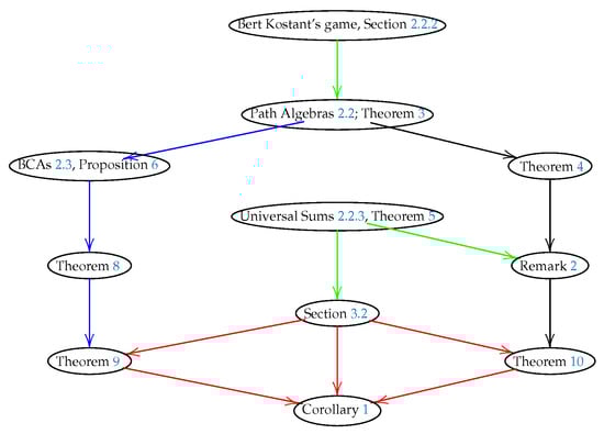
Figure 1. Brauer configuration algebras, Bert Kostant’s game, and mixed sums of square and triangular numbers allow finding main results in this paper. Theorem 9 gives formulas for dimensions of Brauer configuration algebras and corresponding centers associated with the introduced wargame. Such a theorem allows establishing whether a launch of a ground base detector succeeds or fails to detect a missile launched by an adversary using universal sums of triangular numbers. Similar results are given in Theorem 10, but instead of using universal sums of triangular numbers, we use universal sums of square numbers. Corollary 1 applies the Legendre–Gauss theorem on sums of three square numbers to determine which conditions allow an adversary to succeed in the proposed wargame.

2. Background and Related Work

In this section, we introduce some definitions and notations to be used throughout the paper. In particular, a brief overview regarding wargames, Brauer configuration algebras, quadratic forms associated with graphs, and the Cauchy’s polygonal number theorem is given.

Henceforth, the symbol $\mathbb{F}$ will denote a field, $\mathbb{N}$ is the set of natural numbers, and $t_n$ ($s_n$) denotes the nth triangular number (nth square number).

2.1. Wargames

A wargame may be understood as a strategy to reveal and overcome possible weaknesses of players in an armed confrontation. Its history goes back to the origin of civilization. Games Go and Chess are two ancestors of wargames. From these abstract games, several types of war games appeared. One of them is the medieval game Metroxia, a Chess evolution, which simulates a medieval battle between two armies with castles, and a resolution based on mathematics. Around 1644 C, Weikmann in Prussia created a battleground simulation named the Koenigspiel (King’s game). The word wargame has its origin in the German word Kriegsspiel, given to a game introduced in the 19th century by the Prussian army. Kriegspiel is considered the first game used for training and research [14].

The four basic elements of a wargame are [15,16]:

• The game board (map): a wargame-scaled map or landscape from an actual map, where the game pieces are located and labeled according to their properties. Often, a grid is used for a more accurate location of the game components.
• The scenario: a detailed description of the operational environment and situation.
• The rules: wargame rules are the restrictions imposed on the movements of the pieces in the game.
• The adjudication method: the process of determining outcomes in the game.

Recently, Tryhorn et al. [11] introduced a wargame associated with a combinatorial problem. According to them, a bomber crew navigates through enemy territory to reach an objective or target. The contested area is a tiled board. Each tile has a $x-y$ coordinate and an identifier of whether it is neutral, enemy territory, or the target. The goal of the bomber crew consists of reaching the objective without entering enemy territory and keeping it safe from surface to air missiles (SAM) sites. At least one path exists from the start point to the target satisfying the constraints. Finding the number of available paths is a discrete optimization problem (DOP), for which the length of the path is the cost function. The goal of this problem is to find an optimal solution $s_w\in S$, such that $f\left(s_w\right)\le f\left(x\right)$, for all $x\in S$. In general, DOPs are NP-hard problems. Figure 2 shows an example of this wargame scenario. In this case, directed paths are examples of how enemy’s launches can intercept the bomber. The green line identifies the shortest path to reach the target without the enemy’s detection.

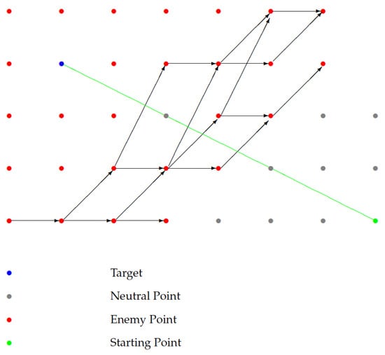
Figure 2. Example of a safe path (green line) according to the Tryhorn et al. model.

2.2. Path Algebras and Quadratic Forms

This section is focused on the theory of representation of finite-dimension algebras associated with finite connected quivers (oriented graphs). We recall relationships between quadratic forms and the classification of algebras [4,6,17,18].

A quiver Q is an oriented graph defined by a quadruple of the form $(Q_0,Q_1,s,t)$, consisting of two sets, $Q_0$ and $Q_1$, and two maps, $s,t:Q_1\to Q_0$; elements of the set, $Q_0$ ($Q_1$), are said to be the vertices (arrows) of the quiver Q.

If $\alpha \in Q_1$, then the vertex, $s\left(\alpha \right)$ ($t\left(\alpha \right)$), is the source (target) of the arrow, $\alpha$ [6].

A path, P, of length, $l\ge 1$, of a quiver, Q, is a sequence of arrows, $P=(a\mid {\alpha }_1,{\alpha }_2,\dots ,{\alpha }_l\mid b)$, where $a={\alpha }_0$, $b={\alpha }_{l+1}$, and $t\left({\alpha }_i\right)=s\left({\alpha }_{i+1}\right)$, $0\le i\le l$, $s\left(a\right)$ ($t\left(b\right)$) is said to be the source (target) of the path, P. Vertices are paths of length 0. If $Q^l$ is the set of all paths of length $l\ge 0$, then we let $\mathcal{Q}={\displaystyle \bigcup _{l\ge 0}}{Q}^l$ denote the set of all paths contained in Q.

An ideal I of a path algebra $\mathbb{F}Q$ is generated by relations. These relations are nothing but paths with the same starting and ending points. The two-sided ideal generated by the arrows (paths of length $\ge l$) of Q is denoted by $R_Q$ ($R_Q^l$). An ideal, I, is said to be admissible, if there is $m\ge 2$, such that $R_Q^m\subseteq I\subseteq R_Q^2$. $R_Q$ is said to be the arrow ideal of $\mathbb{F}Q$.

An algebra, A, is said to be basic if it has a complete set of primitive orthogonal idempotents. Gabriel [19] proved that if an algebra, A, is basic, then there is a quiver, Q, and an admissible ideal, I, such that A is isomorphic to a quotient of the form $\mathbb{F}Q/I$.

If I is an admissible ideal of $\mathbb{F}Q$, then the pair $(Q,I)$ is said to be a bound quiver. The quotient algebra $\mathbb{F}Q/I$ is said to be a bound quiver algebra [4,6].

2.2.1. Quadratic Forms

A quadratic form $q=q(x_1,x_2,\dots ,x_n)$ in n indeterminates $x_1,x_2,\dots ,x_n$ is said to be an integral quadratic form, if it is of the following form:

$$q(x_1,x_2,\dots ,x_n)={\displaystyle \underset{i=1}{\sum ^n}}{x}_i^2+{\displaystyle \sum _{i<j}}{a}_{ij}{x}_i{x}_j$$

(1)

where $a_{ij}\in \mathbb{Z}$ for all $i,j$.

A vector $x={[x_1,x_2,\dots ,x_n]}^T\in {\mathbb{Z}}^n$ is called positive if $x\ne 0$ and $x_j\ge 0$, for all j, $1\le j\le n$. If a vector x is positive, then we write $x>0$ [6,18]. $X^T$ denotes the transpose of a matrix X.

An integral quadratic form q is called weakly positive if $q\left(x\right)>0$, for any vector $x>0$. q is positive semi-definite if $q\left(x\right)\ge 0$, for any $x\in {\mathbb{Z}}^n$. It is positive if $q\left(x\right)>0$ for any $x\ne 0$.

A vector $x\in {\mathbb{Z}}^n$ such that $q\left(x\right)=1$ is called a root.

If Q is a quiver, then the quadratic form of Q denoted $q_Q\left(x\right)$ (or simply q if no confusion arises) has the following form:

$$q_Q\left(x\right)={\displaystyle \sum _{i\in Q_0}}{x}_i^2-{\displaystyle \sum _{\alpha \in Q_1}}{x}_{s\left(t\right)}{x}_{t\left(\alpha \right)}.$$

(2)

If Q is a finite acyclic connected quiver, and $A=\mathbb{F}Q$ is a path algebra, then the Euler quadratic form of A,

$$q_A\left(x\right)={\displaystyle \sum _{i\in Q_0}}{x}_i^2-{\displaystyle \sum _{i,j\in Q_0}}{a}_{ij}{x}_i{x}_j,a_{ij}={\dim }_{\mathbb{F}}{\mathrm{Ext}}_A^1(s\left(i\right),s\left(j\right))$$

(3)

coincides with the quadratic form $q_Q\left(x\right)$ of Q.

For instance, the quadratic form of the quiver

$$Q={\displaystyle \underset{1}{\circ }}⟶{\displaystyle \underset{2}{\circ }}$$

(4)

is given by the identity $q_Q(x_1,x_2)=x_1^2+x_2^2-x_1{x}_2$, in this case, ${\dim }_{\mathbb{F}}{\mathrm{Ext}}_A^1(s\left(1\right),s\left(2\right))=1$. Note that, $(1,0)$, $(0,1)$, and $(1,1)$ are positive roots of $q_Q(x_1,x_2)$.

The reflection $s_i:{\mathbb{Q}}^n\to {\mathbb{Q}}^n$ at a vertex i of a finite connected and acyclic quiver Q is given by the following formula:

$$s_i\left(x\right)=x-2(x,e_i)e_i.$$

(5)

In terms of the coordinates of $x=(x_1,x_2,\dots ,x_n)$, we see that $y=s_i\left(x\right)$ has coordinates:

$$y_j=\left\{\begin{array}{cc}{x}_j,\hfill & \mathrm{if}j\ne i,\hfill \\ -x_i+{\displaystyle \sum _{k-i}}{x}_k,\hfill & \mathrm{if}j=i.\hfill \end{array}\right.$$

The Weyl group, $W_Q$ of a quiver Q, is the automorphisms group of $E={\mathbb{Q}}^n$ generated by the reflections ${\left\{s_i\right\}}_{i\in Q_0}$.

As an example, The following are the matrix representations of the reflections $s_1$ and $s_2$, defined for the quiver (4):

$$s_1=\left[\begin{array}{cc}-1& 1\\ 0& 1\end{array}\right],s_2=\left[\begin{array}{cc}1& 0\\ 1& -1\end{array}\right].$$

(6)

The Coxeter transformation, $c:{\mathbb{Q}}^n\to {\mathbb{Q}}^n$ of a quiver Q ($\{a_1,a_2,\dots ,a_n\}$ is an admissible numbering of the vertices of Q) is given by the following product:

$$c=s_{a_n}{s}_{a_{n-1}}\dots s_{a_2}{s}_{a_1}.$$

(7)

The matrix $M\left(c\right)$ of the Coxeter transformation c in the canonical basis of ${\mathbb{Q}}^n$ is the Coxeter matrix ${\mathsf{\Phi }}_{\mathbb{F}Q}$ of the path algebra associated with Q, which is a useful tool to describe indecomposable $\mathbb{F}Q$-modules. In particular, if ${\left\{e_i\right\}}_{1\le i\le n}$ is the canonical basis of ${\mathbb{Q}}^n$, then the dimension $\dim P\left(i\right)=P_i$ of the projective module associated with the vertex $i\in Q_0$ is given by the following formula:

$$P_i=\dim P\left(i\right)=s_1\dots s_{i-1}\left(e_i\right).$$

(8)

A similar formula can be used for the dimension of injective modules.

${\mathsf{\Phi }}_{\mathbb{F}Q}=-C^{-T}C$, where C is the Cartan matrix associated with the algebra $\mathbb{F}Q$ whose columns are given by the dimension vectors $P_i$.

If $m_i$ is the least integer such that $c^{-m_i-1}{P}_i\neg >0$, then the set $\{c^{-s}{P}_i\mid 1\le i\le n,0\le s\le m_i\}$, equals the set of all positive roots of $q_Q$.

The following results regarding relationships between integral quadratic forms and the classification of algebras were given by Ovsienko, Drozd, and Gabriel, respectively [18,20,21].

Theorem 1

(cf. [18], Theorem 1). If $x=(x_1,x_2,\dots ,x_n)$ is a positive root of a weakly positive integral quadratic form, then the $x_i\le 6$, for all i.

Theorem 2

(cf. [18], p. 3). A weakly positive integral quadratic form q has only finitely many positive roots.

Theorem 3

(cf. [6], Theorem 5.10). If $A=\mathbb{F}Q$ is a path $\mathbb{F}$-algebra of a Dynkin graph $\overline{Q}$ (whose quadratic form $q_{\overline{Q}}$ is weakly positive), then the following are true:

(1)

The mapping $\dim :M\to \dim M$, induces a bijection of indecomposable A-modules and the set of positive roots of the quadratic form $q_Q$ of Q.

(2)

An algebra $A=\mathbb{F}Q$ is representation-finite if its underlying graph $\overline{Q}$ is one of the laced Dynkin diagrams ${\mathbb{A}}_n$, ${\mathbb{D}}_n$, $n\ge 4$, ${\mathbb{E}}_6$, ${\mathbb{E}}_7$, and ${\mathbb{E}}_8$.

For instance, the quadratic form of the Dynkin graph ${\mathbb{E}}_8$ (shown in Figure 3) is positive definite, and there is a unique maximal positive root, namely:

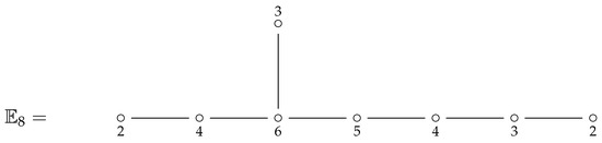
Figure 3. Maximal positive root of the exceptional Dynkin diagram ${\mathbb{E}}_8$.

Remark 1.

We also note that, if the underlying graph, $\overline{Q}$, of a quiver, Q, is a Euclidean graph, $\widetilde{{\mathbb{A}}_n}$, $\widetilde{{\mathbb{D}}_n}$, $\widetilde{{\mathbb{E}}_6}$, $\widetilde{{\mathbb{E}}_7}$, $\widetilde{{\mathbb{E}}_8}$, then $\mathbb{F}Q$ is representation-infinite, and that $q_Q$ is positive semi-definite but not positive definite.

2.2.2. Bert Kostant’s Game and Some of Its Variations

In this section, we describe Gabriel’s Theorem 3 in terms of Bert Kostant’s game.

Postnikov [5] defined Bert Kostant’s game as follows:

1.

For $i\in V$, let $N\left(i\right)$ be the neighbors (adjacent vertices) of i.

2.

For each $i\in V$, we have $c_i\ge 0$ chips, the vector

$${\left(c_i\right)}_{1\le i\le n}=(c_1,c_2,\dots ,c_n)$$

is called a configuration.

3.

A vertex $i\in V$ is said to be:

(a)

Happy if $c_i=\frac{1}{2}{\displaystyle \sum _{j\in N\left(i\right)}}{c}_i$;

(b)

Unhappy if $c_i<\frac{1}{2}{\displaystyle \sum _{j\in N\left(i\right)}}{c}_i$;

(c)

Excited if $c_i>\frac{1}{2}{\displaystyle \sum _{j\in N\left(i\right)}}{c}_i$.

4.

Gaming: Initially $c_i=0$, for all i, $1\le i\le n$ (i.e., all vertices are happy).

Then, we place a chip at a vertex $i_0$, so $i_0$ is excited but its neighbors are unhappy. Subsequently, apply the reflection$c_i⟶-c_i+{\displaystyle \sum _{j\in N\left(i\right)}}{c}_j$ to an unhappy vertex i.

5.

Goal. Make every vertex $i\in V$ happy or excited.

Figure 4 shows how Bert Kostant’s game works to find out the maximal positive root $(1,1,1,1)$ of $q_{{\mathbb{A}}_4}={\displaystyle \underset{i=1}{\sum ^4}}{x}_i^2-x_1{x}_2-x_2{x}_3-x_3{x}_4$ associated with the Dynkin diagram ${\mathbb{A}}_4$ [5].

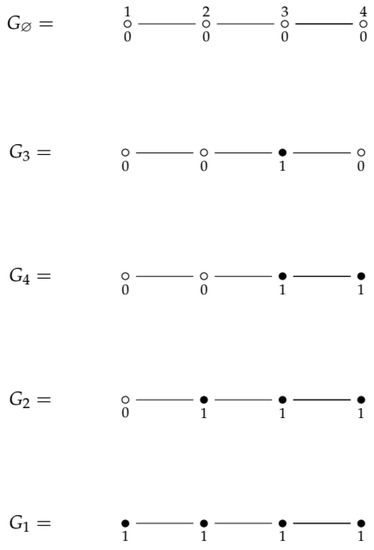
Figure 4. We apply Bert Kostant’s game to the Dynkin diagram ${\mathbb{A}}_4$. Symbol $G_i$, $1\le i\le 4$, means that vertex i of the Dynkin diagram ${\mathbb{A}}_4$ receives one chip (associated vertices are black). $G_{⌀}$ means that no vertex of the diagram receives a chip (associated vertices are all blank).

A graph G is of finite type if Bert Kostant’s game ends.

The following proposition was proved by Postnikov:

Proposition 1

([5], Proposition 1.3.). Suppose that there is a way to play until the game ends. Then, any sequence of moves eventually leads to a terminating state. Moreover, if the final configuration vector does not depend on the choice of moves, nor the initial vertex, then we add a chip on.

Proposition 2.

Bert Konstant’s game does not terminate if G is an n-star (i.e., an n-star is of infinite type).

Proof. 

If the movements are applied first to vertices $\{1,2,\dots ,n-1\}$, then the configuration $c=(c_1,c_2,\dots ,c_{n-1},c_n)$, associated with the $(n^2-n+1)$th stage of the game, has the following form: $(n,n,\dots ,n,n)$. Thus, vertex n is unhappy and the remaining vertices are excited.    □

The chip-firing game is the first variation of Bert Kostant’s game introduced by Postnikov [5]. Its definition goes as follows:

1.

Let $c=(c_1,c_2,\dots ,c_n)$ be a configuration associated with a graph

$G=(V=[n],E)$. Then, a vertex $i\in V$ is said to be stable (unstable) if $c_i<{\mathrm{deg}}_G\left(i\right)$ ($c_i\ge {\mathrm{deg}}_G\left(i\right)$).

2.

Gaming.

(a)

Pick an unstable vertex i and move a chip to each of its neighbors.

(b)

Extend graph $G=(V,E)$ to the graph $G^{*}=(V^{*}=V\cup \{\ast \},E^{*}=E\cup M_{*})$, where ∗ is a sink vertex, which eats all chips fired at it.

3.

Goal: Make every vertex $i\in V$ stable.

Proposition 3.

Chip-firing games with a sink always terminate.

The following Cartan-firing game is defined as the chip-firing game but instead of using the degree of a vertex i, it uses the number two.

1.

Let $c=(c_1,c_2,\dots ,c_n)$ be a configuration associated with a graph $G=(V=[n],E)$. Then, a vertex $i\in V$ is said to be stable (unstable) if $c_i\in \{0,1\}$ ($c_i\ge 2$).

2.

Gaming.

(a)

Pick an unstable vertex, i, and move two chips to each of its neighbors (the assignment $c_i\to c_i-2$ holds).

(b)

The assignment $c_j\to c_j+1$ holds for each neighbor j of i.

3.

Goal: Make every vertex $i\in V$ stable.

Proposition 4

([5], Proposition 1.7). If G is a path, then the Cartan-firing game terminates.

Let $A=\left(a_{ij}\right)$ be an $n\times n$-symmetric matrix, such that $a_{ii}>0$ and $a_{ij}<0$, if $i\ne j$.

If $A_i$ denotes the ith row of the matrix A and $c=(c_1,c_2,\dots ,c_n)>0$ is a configuration, then the assignment $c\to c-A_i$, if $c_i\ge a_{ii}$ constitutes a firing move in a matrix-firing game.

The following proposition was also proved by Postnikov.

Proposition 5

([5], Proposition 2.7). Let A be a matrix satisfying the constraints of a matrix-firing game. Then, the following assertions are equivalent:

• The A-firing is finite for any initial configuration.
• There exists a vector, $h=(h_1,h_2,\dots ,h_n)>0$, such that $Ah>0$.
• A is positive definite.

A configuration, $h>0$, is said to be a Vinberg function, if $Ah=0$. It is a sub-additive function if $Ah\ge 0$ (which means that h is happy or excited). h is a strictly sub-additive function if $Ah>0$ (i.e., h is excited).

The following theorem can be considered Bert Kostant’s game version of Gabriel’s Theorem 3 (see also Remark 1). It gives relationships between the aforementioned games and the theory of representation of finite-representation algebras [5].

Theorem 4

([5], Theorem 4.9). The following statements are equivalent for a graph, G:

• Kostant’s game is finite.
• Cartan’s firing game is finite for any initial configuration.
• The Cartan matrix $A=A_G=2I-\mathrm{Adj}\left(A\right)$ is positive definite.
• All principal minors of A are nonzero.
• There exists a strictly sub-additive function $h>0$ on G.
• G is isomorphic to one of the laced Dynkin diagrams.
• G has no subgraph isomorphic to any Euclidean diagram.

2.2.3. Universal Mixed Sums of Square and Triangular Numbers

This section briefly describes advances in the research of two lines of investigation founded by Fermat in 1654 and Ramanujan in 1916 [13,22,23,24,25].

Firstly, we recall that Fermat, in a letter written to Pascal, claimed that any number can be written as a sum of at most k, k-gonal numbers (i.e., any number is a triangular number, it is a sum of two triangular or the sum of three triangular numbers; any number is a square number, a sum of two, three, or four square numbers; furthermore, and so on, to infinity [13,23]). Cauchy proved this assertion in 1813. Nathanson [24] gave a short proof of this result in 1987.

Before Cauchy’s theorem proof, several crucial results appeared. For instance, in 1772, Lagrange proved that any number can be written as a sum of four square numbers. According to Nathanson [24], this result is the backbone of the additive number theory.

In 1798, Legendre proved that no number of the form $4^m(8n+7)$ can be written as a sum of three square numbers. In 1801, Gauss went beyond Legendre, by proving this result using the theory of ternary quadratic forms.

In 1862, Liouville proved the following theorem:

Theorem 5

(Liouville, 1862; cf. [26] (1, p. 23)). Let $a,b,c\in {\mathbb{Z}}^{+}$ and $a\le b\le c$. Then, any $n\in \mathbb{N}$ can be written in the form $a{t}_x+b{t}_y+c{t}_z$, if—and only if—the following is true: $(a,b,c)$ is among

$$(1,1,1),(1,1,2),(1,1,4),(1,1,5),(1,2,2),(1,2,3),(1,2,4).$$

The second line of investigation was founded in 1916 by Ramanujan [25], who conjectured that there are 55 quadruples $(a,b,c,d)\in {\mathbb{Z}}^4$ with $a\le b\le c\le d$, such that each $n\in \mathbb{N}$ can be written as $a{x}^2+b{y}^2+c{z}^2+d{w}^2$, with $x,y,z,w\in \mathbb{Z}$.

In 1927, Dickson confirmed that 54 of the quadruples proposed by Ramanujan were right. As a message for the future, only one $(1,2,5,5)$ was incorrect (it does not represent 15).

In 1993, Conway and Schneeberger conjectured the following result (known as the fifteen theorem), elegantly proved by Bhargava in 2000 [22,27].

Theorem 6

(Fifteen Theorem; [27], Theorem 1). If a positive integer-matrix quadratic form represents each of 1, 2, 3, 5, 6, 7, 10, 14, 15, then it represents all positive integers.

Remark 2.

Between 2005 and 2010, Sun et al. proved that the following list of sums is universal [28,29,30,31,32]:

$t_x+t_y+z^2$, $t_x+t_y+2z^2$, $t_x+t_y+4z^2$, $t_x+2t_y+z^2$, $t_x+2t_y+2z^2$, $t_x+2t_y+3z^2$, $t_x+2t_y+4z^2$, $2t_x+t_y+z^2$, $2t_x+4t_y+z^2$, $2t_x+5t_y+z^2$, $t_x+3t_y+z^2$, $t_x+4t_y+z^2$, $t_x+4t_y+2z^2$, $t_x+6t_y+z^2$, $t_x+8t_y+z^2$, $t_x+y^2+z^2$, $t_x+y^2+2z^2$, $t_x+y^2+3z^2$, $t_x+y^2+4z^2$, $t_x+y^2+8z^2$, $t_x+2y^2+2z^2$, $t_x+2y^2+4z^2$, $2t_x+y^2+z^2$, $2t_x+y^2+2z^2$, $4t_x+y^2+2z^2$.

In 2009, Kane [30] proved the following result, known as the eight theorem.

Theorem 7

([30], Theorem 1.1).

Fix the sequence $b_1\le b_2\le \dots \le b_k\in \mathbb{N}$. Then,

1.

The sum of triangular numbers

$$f\left(x\right)=f_b\left(x\right)={\displaystyle \underset{i=1}{\sum ^k}}{b}_i{t}_{x_i}$$

represents every positive integer if—and only if—$f_b$ represents the integers $1,2,4,5,$ and 8.

2.

The corresponding diagonal quadratic form $Q\left(x\right)={\displaystyle \underset{i=1}{\sum ^k}}{b}_i{s}_{x_i}$ with $x_i$ all odd represents every integer of the form

$$8n+{\displaystyle \underset{i=1}{\sum ^k}}{b}_i, n\ge 0$$

if—and only if—it represents $8+{\displaystyle \underset{i=1}{\sum ^k}}{b}_i$, $16+{\displaystyle \underset{i=1}{\sum ^k}}{b}_i$, $32+{\displaystyle \underset{i=1}{\sum ^k}}{b}_i$, $40+{\displaystyle \underset{i=1}{\sum ^k}}{b}_i$, and $64+{\displaystyle \underset{i=1}{\sum ^k}}{b}_i$.

2.3. Brauer Configuration Algebras

In this section, we discuss some results regarding Brauer configuration algebras introduced by Green and Schroll in [1].

A Brauer configuration algebra ${\mathsf{\Lambda }}_{\mathsf{\Gamma }}$ (or simply $\mathsf{\Lambda }$ if no confusion arises) is induced by a Brauer configuration $\mathsf{\Gamma }=({\mathsf{\Gamma }}_0,{\mathsf{\Gamma }}_1,\mu ,\mathcal{O})$, where:

• ${\mathsf{\Gamma }}_0$ is a finite set of vertices.
• ${\mathsf{\Gamma }}_1$ is a collection of polygons, which are multisets, consisting of vertices (vertices repetition allowed), ${\mathsf{\Gamma }}_1=\{U_i\mid 1\le i\le n\}$ for some suitable integer, n. Any polygon, $U_i$, contains more than one vertex.
• $\mu$ is a map from the set of vertices, ${\mathsf{\Gamma }}_0$, to the set of positive integers $\mathbb{N}\backslash \left\{0\right\}={\mathbb{N}}^{+}$, $\mu :{\mathsf{\Gamma }}_0\to {\mathbb{N}}^{+}.$
• $\mathcal{O}$ is an ordering < defined on ${\mathsf{\Gamma }}_1$. Such ordering is a way of registering how vertices occur in polygons. For instance, if a vertex $\alpha \in {\mathsf{\Gamma }}_0$ occurs in polygons $U_{i_i},U_{i_2},\dots ,U_{i_m}$, for suitable indices $i_1,i_2,\dots ,i_m\in \{1,2,3,\dots ,n\}$, then the ordering, <, can be defined in such a way that:

  $$U_{i_1}^{{\alpha }_1}<U_{i_2}^{{\alpha }_2}<\dots <U_{i_m}^{{\alpha }_m},{\alpha }_{i_s}>0.$$

  (9)

  where $U_{i_s}^{{\alpha }_s}=\underset{{\alpha }_s-times}{\underbrace{U_{i_s}<\dots <U_{i_s}}}$ means that vertex $\alpha$ occurs ${\alpha }_s$ in polygon $U_{i_s}$, denoted $occ(\alpha ,U_{i_s})$.
  The sequence (9) is said to be the successor sequence at vertex $\alpha$, denoted $S_{\alpha }$. Note that, for the sake of clarity, if a vertex ${\alpha }^{\prime }\ne \alpha$ also occurs in polygons $U_{i_i},U_{i_2},\dots ,U_{i_m}$, then we keep such polygons ordering if it has already been defined.
• If $\alpha \in {\mathsf{\Gamma }}_0$, then there is at least one polygon, $U_i$, such that $\alpha \in U_i$.

If $\alpha \in {\mathsf{\Gamma }}_0$, then the valency, $val\left(\alpha \right)$, of $\alpha$ is given by the following identity:

$$val\left(\alpha \right)={\displaystyle \sum _{U\in {\mathsf{\Gamma }}_1}}occ(\alpha ,U).$$

(10)

If $\alpha \in {\mathsf{\Gamma }}_0$ is such that $\mu \left(\alpha \right)val\left(\alpha \right)=1$, then $\alpha$ is said to be truncated (it occurs once in just one polygon). Otherwise, $\alpha$ is a non-truncated vertex. A Brauer configuration without truncated vertices is said to be reduced.

In [17], Cañadas et al. introduced Algorithm 1 to build the Brauer quiver $Q_{\mathsf{\Gamma }}$ and the Brauer configuration algebra ${\mathsf{\Lambda }}_{\mathsf{\Gamma }}=\mathbb{F}{Q}_{\mathsf{\Gamma }}/I_{\mathsf{\Gamma }}$ induced by the Brauer configuration $\mathsf{\Gamma }$, where $I_{\mathsf{\Gamma }}$ is an admissible ideal generated by suitable relations associated with the vertices occurrences.    

Algorithm 1: Construction of a Brauer configuration algebra.

1. Input A reduced Brauer configuration $\mathsf{\Gamma }=({\mathsf{\Gamma }}_0,{\mathsf{\Gamma }}_1,\mu ,\mathcal{O})$. 2. Output The Brauer configuration algebra ${\mathsf{\Lambda }}_{\mathsf{\Gamma }}=\mathbb{F}{Q}_{\mathsf{\Gamma }}/I_{\mathsf{\Gamma }}$. 3. Construct the quiver $Q_{\mathsf{\Gamma }}=({\left(Q_{\mathsf{\Gamma }}\right)}_0,{\left(Q_{\mathsf{\Gamma }}\right)}_1,s:{\left(Q_{\mathsf{\Gamma }}\right)}_1\to {\left(Q_{\mathsf{\Gamma }}\right)}_0,t:{\left(Q_{\mathsf{\Gamma }}\right)}_1\to {\left(Q_{\mathsf{\Gamma }}\right)}_0)$. (a) ${\left(Q_{\mathsf{\Gamma }}\right)}_0={\mathsf{\Gamma }}_1$, (b) For each cover $U_i<U_{i+1}\in {\mathsf{\Gamma }}_1$, define an arrow $a\in {\left(Q_{\mathsf{\Gamma }}\right)}_1$, such that $s\left(a\right)=U_i$ and $t\left(a\right)=U_{i+1}$; (c) Each relation $U_i<U_i$ defines a loop in $Q_{\mathsf{\Gamma }}$; (d) Each ordered set $S_{\alpha }$ defines a cycle $C_{\alpha }=S_{\alpha }\cup \{U_{i_m}<U_{i_1}\}$ in $Q_{\mathsf{\Gamma }}$; called special cycles. Special cycles are obtained from successor sequences by defining a suitable circular relation, without loss of generality, we assume that a relation of the form $U_{i_m}<U_{i_1}$ holds in special cycles. 4. Define the path algebra $\mathbb{F}{Q}_{\mathsf{\Gamma }}$; 5. Construct the admissible ideal $I_{\mathsf{\Gamma }}$, which is generated by the following relations: (a) If ${\alpha }_i,{\alpha }_j\in U$, $U\in {\mathsf{\Gamma }}_1$ and $C_{{\alpha }_i},C_{{\alpha }_j}$ are corresponding special cycles, then $C_{{\alpha }_i}^{\mu \left({\alpha }_i\right)}-C_{{\alpha }_j}^{\mu \left({\alpha }_j\right)}=0$; (b) If $C_{{\alpha }_i}$ is a special cycle associated with the vertex ${\alpha }_i$, then $C^{\mu \left({\alpha }_i\right)}a=0$, if a is the first arrow of $C_{{\alpha }_i}$; (c) If $\alpha ,{\alpha }^{\prime }\in {\mathsf{\Gamma }}_0$, $\alpha \ne {\alpha }^{\prime }$, $a,b\in {\left(Q_{\mathsf{\Gamma }}\right)}_1$, $a\ne b$, $ab\notin C_{\alpha }$ for any $\alpha \in {\mathsf{\Gamma }}_0$, then $ab=0$, if $a\in C_{\alpha }$, $b\in C_{{\alpha }^{\prime }}$ and $ab\in \mathbb{F}{Q}_{\mathsf{\Gamma }}$; (d) If a is a loop associated with a vertex $\alpha$ with $val\left(\alpha \right)=1$ and $\mu \left(\alpha \right)>1$, then $a^{\mu \left(\alpha \right)+1}=0$. 6. ${\mathsf{\Lambda }}_{\mathsf{\Gamma }}=\mathbb{F}{Q}_{\mathsf{\Gamma }}/I_{\mathsf{\Gamma }}$ is the Brauer configuration algebra; 7. For the construction of a basis of ${\mathsf{\Lambda }}_{\mathsf{\Gamma }}$, follow the next steps: (a) For each $U\in {\mathsf{\Gamma }}_1$, choose a non-truncated vertex, ${\alpha }_U$, and exactly one special $\alpha$-cycle $C_{{\alpha }_U}$ at U, (b) Define: $$\begin{array}{cc}\hfill A& =\{\overline{p}\mid pisaproperprefixofsome{C}_{\alpha }^{\mu \left(\alpha \right)}\},\hfill \\ \hfill B& =\{\overline{C_{{\alpha }_U}^{\mu \left(\alpha \right)}}\mid U\in {\mathsf{\Gamma }}_1\}.\hfill \end{array}$$ (c) $A\cup B$ is a $\mathbb{F}$-basis of ${\mathsf{\Lambda }}_{\mathsf{\Gamma }}$.

Henceforth, if no confusion arises, we will assume notations Q, I and $\mathsf{\Lambda }$ instead of $Q_{\mathsf{\Gamma }}$, $I_{\mathsf{\Gamma }}$, and ${\mathsf{\Lambda }}_{\mathsf{\Gamma }}$, for a quiver, an admissible ideal, and the Brauer configuration algebra induced by a fixed Brauer configuration, $\mathsf{\Gamma }$.

The following Proposition 6 and Theorem 8 give formulas for the dimension and the center of a Brauer configuration algebra [1,2].

Proposition 6

([1], Proposition 3.13). Let Λ be a Brauer configuration algebra associated with the Brauer configuration Γ, and let $\mathcal{C}=\{C_1,\dots ,C_t\}$ be a full set of equivalence class representatives of special cycles. Assume that for $i=1,\dots ,t$, $C_i$ is a special ${\alpha }_i$-cycle, where ${\alpha }_i$ is a non-truncated vertex in Γ. Then,

$${\dim }_{\mathbb{F}}\mathsf{\Lambda }=2|Q_0|+{\displaystyle \sum _{C_i\in \mathcal{C}}}|C_i\left|\right(n_i|C_i|-1),$$

where $|Q_0|$ denotes the number of vertices of Q, $|C_i|$ denotes the number of arrows in the ${\alpha }_i$-cycle $C_i$ and $n_i=\mu \left({\alpha }_i\right)$.

Theorem 8

([2], Theorem 4.9). Let Γ be a reduced and connected Brauer configuration and let Q be its induced quiver and let Λ be the induced Brauer configuration algebra, such that ${\mathrm{rad}}^2\mathsf{\Lambda }\ne 0$, then the dimension of the center of Λ denoted ${\dim }_{\mathbb{F}}Z\left(\mathsf{\Lambda }\right)$ is given by the following formula:

$$\begin{array}{cc}\hfill {\dim }_{\mathbb{F}}Z\left(\mathsf{\Lambda }\right)& =1+{\displaystyle \sum _{\alpha \in {\mathsf{\Gamma }}_0}}\mu \left(\alpha \right)+|{\mathsf{\Gamma }}_1|-|{\mathsf{\Gamma }}_0|+\#\left(LoopsQ\right)-|{\mathcal{C}}_{\mathsf{\Gamma }}|,\hfill \end{array}$$

where $|{\mathcal{C}}_{\mathsf{\Gamma }}|=\{\alpha \in {\mathsf{\Gamma }}_0\mid val\left(\alpha \right)=1,and\mu \left(\alpha \right)>1\}$.

In this case, $\mathrm{rad}M$ denotes the radical of a module, M, $\mathrm{rad}M$ is the intersection of all the maximal submodules of M.

3. Main Results

In this section, we define a wargame as a variation of Bert Kostant’s game, whose outcomes can be described in terms of mixed sums of triangular and square numbers. Such a wargame induces a Brauer configuration associated with points of $\mathbb{N}\times \mathbb{N}$. Dimensions of these algebras and their corresponding centers are estimated.

3.1. Admissible Paths and the Left Boundary Path

Let us consider a quiver, $Q(a,b,c)=(Q_0,Q_1,s,t)$, where the following are true:

• $Q_0\subset {\mathbb{N}}^2$,
• Any arrow $\alpha \in Q_1$ belongs to a product of at most three admissible paths, ${\mathcal{A}}_1^a$ (the left boundary path (l.b.p), ${\mathcal{A}}_2^b$, ${\mathcal{A}}_3^c$, $a>0$, and $b,c$ are non-negative integers. The symbol ${\mathcal{A}}_j^0$ for $j\in \{2,3\}$ means that the path ${\mathcal{A}}_j$ does not appear in the product. Moreover, ${\mathcal{A}}_j^0{\mathcal{A}}_{j^{\prime }}^{i^{\prime }}={\mathcal{A}}_{j^{\prime }}^{i^{\prime }}{\mathcal{A}}^0={\mathcal{A}}_{j^{\prime }}^{i^{\prime }}$.
• ${\mathcal{A}}_j^i$ denotes a path product of i copies of ${\mathcal{A}}_j$, whose set of arrows, $\{{\alpha }_{1,1}^a,{\alpha }_{1,2}^a,\dots ,{\alpha }_{1,n_1}^a\}$, $\{{\beta }_{2,1}^b,{\beta }_{2,2},{\beta }_{2,n_2}\}$, and $\{{\gamma }_{3,1}^c,{\gamma }_{3,2}^c,{\gamma }_{3,n_3}^c\}$, respectively, satisfy the following properties:

  1.

  $n_3\le n_2$,

  2.

  If $m\left({\delta }_{j,t}\right)\in \mathbb{N}$, $\delta \in \{\alpha ,\beta ,\gamma \}$, $1\le j\le 3$ is the slope of an arrow ${\delta }_{j,t}\in {\mathcal{A}}_j$, then $m\left({\delta }_{j,t}\right)=m\left({\delta }_{j,t-1}\right)+1$. In particular, the source $s\left(a_{1,1}\right)=(0,0)$, and $m_{{\alpha }_{1,1}}=m\left({\beta }_{2,1}\right)=m\left({\gamma }_{3,1}\right)=0$.

  3.

  For $i\ge 2$, $1\le r\le n_j$, $1\le j\le 3$, $\delta \in \{\alpha ,\beta ,\gamma \}$, it holds that the set of arrows $\{{\delta }_{j,1}^i,{\delta }_{j,2}^i,\dots ,{\delta }_{j,n_j}\}$ of ${\mathcal{A}}_j^i$ are such that

  $$m\left({\delta }_{j,r}^i\right)=m\left({\delta }_{j,r}\right),\left|\right|{\delta }_{j,r}\left|\right|,t\left({\delta }_{j,n_j}^{i-1}\right)=s\left({\delta }_{j,1}^i\right)$$

  (11)

  for all possible values of i, $\delta$, and j. Furthermore,

  $$\begin{array}{cc}\hfill t({\alpha }_{1,n_1}^a)& =s\left({\beta }_{2,1}\right),t\left({\beta }_{2,n_2}\right)=s\left({\gamma }_{3,1}\right).\hfill \\ \hfill {\alpha }_{1,n_1}^a{\beta }_{2,s}& ={\beta }_{2,n_2}^b{\gamma }_{3,s^{\prime }}={\alpha }_{1,t}^i{\gamma }_{3,t^{\prime }}^{i^{\prime }}={\beta }_{2,u}^l{\alpha }_{1,u^{\prime }}^{l^{\prime }}=0,\hfill \end{array}$$

  (12)

  for $s,s^{\prime }>1$ and all possible values of $i,i^{\prime },l,l^{\prime },t,t^{\prime },u$, and $u^{\prime }$.

  4.

  Two admissible paths, ${\mathcal{A}}_j^i$ and ${\mathcal{A}}_{j^{\prime }}^{i^{\prime }}$, are equivalent, denoted ${\mathcal{A}}_j^i\sim {\mathcal{A}}_{j^{\prime }}^{i^{\prime }}$. If one is obtained from the other via slope permutations (e.g., the admissible path ${\mathcal{A}}_j$ with slopes sequence of the form $\{0,1,0,1,0\}$), then it is equivalent to the admissible path, ${\mathcal{A}}_{j^{\prime }}$, with slopes sequence of the form $\{0,0,1,0,1\}$).

Figure 5 shows examples of admissible paths.

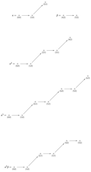
Figure 5. Examples of admissible paths with $(0,0)$ and $(4,2)$ as starting points.

For a fixed positive integer, m, and a non-negative integer, j, let ${\mathcal{L}}_j$ be a subset of ${\mathbb{N}}^2$, such that

$${\mathcal{L}}_j=\{(x,y)\in \mathbb{N}\times \mathbb{N}\mid y=-m(x-j)\}$$

(13)

We let $P_{j,i}$ denote the points of ${\mathcal{L}}_j$, whose coordinates have the form $(i,-m(i-j\left)\right)$.

If $P_{j,i},P_{j,i^{\prime }}\in {\mathcal{L}}_j$, then they are equivalent. Thus, subsets ${\mathcal{L}}_j$ constitute a partition of ${\mathbb{N}}^2$.

Brauer Configuration Algebras Associated with Admissible Paths

For $j>1$ fixed, the set ${\mathfrak{A}}_j$ consisting of all classes of admissible paths ending at points $P_{j,i}$ defines a Brauer configuration, ${\mathsf{\Gamma }}^j=\{{\mathsf{\Gamma }}_0^j,{\mathsf{\Gamma }}_1^j,{\mu }^j,{\mathcal{O}}^j\}$, where

• ${\mathsf{\Gamma }}_0^j=\left[{\nu }_j\right]=\{0,1,2,\dots ,{\nu }_j\}$, ${\nu }_j=\max \{m\left({\delta }_j^i\right)\mid {\delta }_j^i\mathrm{is}\mathrm{an}\mathrm{arrow}\mathrm{of}{\mathcal{A}}_j^i\in {\mathfrak{A}}_j\}$.
• ${\mathsf{\Gamma }}_1^j={\mathfrak{A}}_j$, i.e., polygons are representative of admissible paths classes, whose associated word, $w\left({\mathcal{A}}_j\right)$, is given by the corresponding slope sequence.
• ${\mu }^j\left(s\right)=3$.
• If ${\mathfrak{A}}_j=\{{\mathcal{A}}_{j,1}^{i_1},{\mathcal{A}}_{j,2}^{i_2},\dots ,{\mathcal{A}}_{j,s}^{i_s}\}$, where ${\mathcal{A}}_{j,h}^{i_h}$ denotes a representative of admissible paths, then an ordering ${\mathcal{O}}^j$ is defined in such a way that in successor sequences; thus, it holds that ${\mathcal{A}}_{j,h}^{i_h}<{\mathcal{A}}_{j,h+1}^{i_h+1}$.

For instance, ${\mathsf{\Gamma }}^3=({\mathsf{\Gamma }}_0^3,{\mathsf{\Gamma }}_1^3,{\mu }^3,{\mathcal{O}}^3)$, where

• ${\mathsf{\Gamma }}_0^3=\{0,1\}$;
• ${\mathsf{\Gamma }}_1^3=\{{\mathcal{A}}_{3,1},{\mathcal{A}}_{3,2}\}$;
• $w\left({\mathcal{A}}_{3,1}\right)=01$, $w\left({\mathcal{A}}_{3,2}\right)=000=0^{\left(3\right)}$;
• The orientation ${\mathcal{O}}^3$ is defined in such a way that successor sequences, $S_0$ and $S_1$, and special cycles, $C_0$ and $C_1$, associated with vertices 0 and 1, respectively, have the following form:

  $$\begin{array}{cc}\hfill S_0& ={\mathcal{A}}_{3,1}<{\mathcal{A}}_{3,2}<{\mathcal{A}}_{3,2}<{\mathcal{A}}_{3,2},\hfill \\ \hfill C_0& ={\mathcal{A}}_{3,1}<{\mathcal{A}}_{3,2}<{\mathcal{A}}_{3,2}<{\mathcal{A}}_{3,2}<{\mathcal{A}}_{3,1},\hfill \\ \hfill S_1& ={\mathcal{A}}_{3,1},\hfill \\ \hfill C_1& ={\mathcal{A}}_{3,1}<{\mathcal{A}}_{3,1},\hfill \\ \hfill val\left(0\right)& =4,val\left(1\right)=1,\hfill \\ \hfill \mu \left(0\right)val\left(0\right)& =16,\mu \left(1\right)val\left(1\right)=4.\hfill \end{array}$$

Figure 6 shows the Brauer quiver $Q_{{\mathsf{\Gamma }}^3}$.

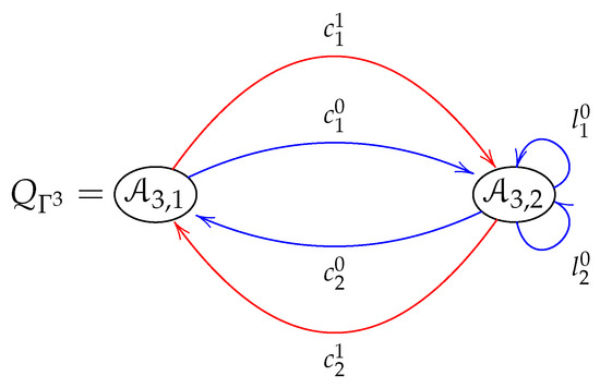
Figure 6. Brauer quiver defined by the Brauer configuration ${\mathsf{\Gamma }}^3$.

The ideal $I_{{\mathsf{\Gamma }}^3}$ associated with the Brauer configuration algebra ${\mathsf{\Lambda }}_{{\mathsf{\Gamma }}^3}=\mathbb{F}{Q}_{{\mathsf{\Gamma }}^3}$ is generated by the following relations:

• $c_1^0{c}_2^0$, $c_j^1{c}_{j^{\prime }}^0$, $c_{j^{\prime }}^0{c}_j^1$, for all possible values of j and $j^{\prime }$.
• ${\left(l_1^0\right)}^4$, ${\left(l_2^0\right)}^4$, $l_j^0{c}_2^1$, $c_1^1{l}_j^0$, $j=1,2$.
• $C_j^{3}a$, if a is the first arrow of a special cycle $C_j$, $j=0,1$.
• $C_0^3\sim C_1^3$.

$$\begin{array}{cc}\hfill {\dim }_{\mathbb{F}}{\mathsf{\Lambda }}_{{\mathsf{\Gamma }}^3}& =4+4(16-1)+1(4-1)=67.\hfill \\ \hfill {\dim }_{\mathbb{F}}Z\left({\mathsf{\Lambda }}_{{\mathsf{\Gamma }}^3}\right)& =1+4\left(2\right)-2+\left(2\right)+1=10.\hfill \end{array}$$

(14)

3.2. A Wargame Associated with Admissible Paths

The wargame we define (admissible path-firing) is similar to how a missile defense system works (MDS). Its definition goes as follows:

1.

Players: Two adversary armies, A and B. Army A has an MDS to protect a region (subset) of ${\mathbb{N}}^2$ from missiles launched by army B.

2.

Gaming:

• Army B launches missiles from a point $(h,0)$, $1\le h\le j$, to a target $T_B$ located at a point $(x,y)$ in a region $R_A\subset {\mathbb{N}}^2$. If the set of vertices of the left boundary path ${\mathcal{A}}_1^a$ is $\{({\displaystyle \underline{x_0}},{\displaystyle \underline{y_0}})=(0,0),({\displaystyle \underline{x_1}},{\displaystyle \underline{y_1}}),\dots ,({\displaystyle \underline{x_t}},{\displaystyle \underline{y_t}})\}$, then for some j, $0\le j\le t$, it holds that $x={\displaystyle \underline{x_j}}$, and $y>y_j$.
• Army A protects a region:

  $$Dome\subseteq \{(x,y)\in {\mathbb{N}}^2\mid 0\le x\le t_1\ge j,0\le y\le t_2\ge j\}$$

  (15)

  with an MDS, which fires admissible paths from a ground-based interceptor (GBI) located at the point $(0,0)$. According to this model, missiles are endowed with a GPS device which makes them a missile trajectory, so that it is possible to consider that the GBI launches admissible paths.
• Missiles launched by army B follow a linear trajectory with slope m. Army A GBI have as goal intercepting launches from army B, reaching points inside the dome.

3.

End of the game: The game is over once army A has launched all admissible paths associated with the class ${\mathcal{L}}_j$, including those with maximal scope (the largest missile scope for which ${\pi }_x\left(P_{x_{t-1},s}\right)\le j\le {\pi }_x\left(P_{x_t,s^{\prime }}\right)$, $P_{x_{t-1},s},P_{x_t,s^{\prime }}\in l.b.p).$

If a missile launched by army B, following a trajectory determined by a class ${\mathcal{L}}_j$, then a GBI launch is said to be

• Happy, if exactly one class of admissible paths (only one shot) reaches ${\mathcal{L}}_j$ (i.e., $|{\mathsf{\Gamma }}_1^j|=1$).
• Unhappy, if no class of admissible paths reaches ${\mathcal{L}}_j$ (i.e., $|{\mathsf{\Gamma }}_1^j|=0$).
• Excited, if more than one class of admissible paths reaches ${\mathcal{L}}_j$ (i.e., $|{\mathsf{\Gamma }}_1^j|>1$).

Problem 1.

For $m,j\ge 1$ fixed. Which values of $a,b$, and c make any launch of the army A to points of classes ${\mathcal{L}}_j$ happy or excited.

Figure 7 shows an example of a happy shot obtained by intercepting a launch from point $B(4,0)$ with $m=1$.

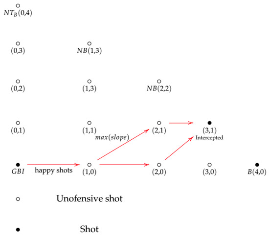
Figure 7. Example of a happy launch intercepting an adversary shot from point $(4,0)$.

The following Theorem 9 gives a solution to the Problem 1. In this case, formulas for the dimension of Brauer configuration algebras ${\mathsf{\Lambda }}_{{\mathsf{\Gamma }}^j}$ and their centers $Z\left({\mathsf{\Lambda }}_{{\mathsf{\Gamma }}^j}\right)$ are obtained via the number of integer partitions $p_{3\Delta }\left(j\right)$ of j into three triangular numbers. Appropriated values of $a,b$, and c in Problem 1 are obtained as a consequence of Theorem 5 regarding universal sums of triangular numbers.

Theorem 9.

If $m=1$ and $j\ge 1$, then

1.

${\dim }_{\mathbb{F}}{\mathsf{\Lambda }}_{{\mathsf{\Gamma }}^j}\le 2p_{3\Delta }\left(j\right)({\nu }_j{p}_{(a+b+c){\nu }_j}^5+1)$, where $p_j^5$ denotes the ith pentagonal number and $p_{3\Delta }\left(j\right)$ denotes the number of partitions of j into at most three triangular numbers.

2.

${\dim }_{\mathbb{F}}Z\left({\mathsf{\Lambda }}_{{\mathsf{\Gamma }}^j}\right)\le 1+3{\nu }_j+p_{3\Delta }\left(j\right)(1+(a+b+c-3){\nu }_j)$.

3.

For corresponding Brauer configurations, it holds that $|{\mathsf{\Gamma }}_1^{27j+12}|=3|{\mathsf{\Gamma }}_1^{3j+1}|$, for any $j\ge 0$.

4.

Any launch to a class ${\mathcal{L}}_j$ is happy or excited if the triplet $(a,b,c)$ is among the following list: $(1,1,1),(1,1,2),(1,1,4),(1,1,5),(1,2,2),(1,2,3),(1,2,4).$

5.

Any launch to a class ${\mathcal{L}}_j$ is happy or excited for a choice of $a,b$, and c if—and only if—it is happy or excited for $j\in \{1,2,4,5,8\}$.

Proof. 

1.

Firstly, note that, as consequence of Theorems 5 and 7, each number $j\in \mathbb{N}$ has associated at least one admissible path. The correspondence goes as follows:

• A triangular number $j=t_x$ is in correspondence with an admissible path $H_j$ of type ${\mathcal{A}}_1$ with source $s\left(H_x\right)=(0,0)$ and target $t\left(H_x\right)=(x,t_{x-1})$.
• If a natural number, j, is a sum of two triangular numbers, i.e., $j=t_x+t_y$ ($y\ge x>0$), then j has associated a path product $H_x{H}_y$ of type ${\mathcal{A}}_2$, such that

  $$\begin{array}{cc}\hfill s\left(H_x\right)& =(0,0),t\left(H_x\right)=(y,t_{y-1}),\hfill \\ \hfill s\left(H_y\right)& =(y,t_{y-1}),t\left(H_y\right)=(x+y,j-(x+y)).\hfill \end{array}$$

  (16)
• If $j\in \mathbb{N}$ is a sum of three triangular numbers with the form $j=t_x+t_y+t_z$ ($z\ge y\ge x>0$), then j corresponds to a path product $H_x{H}_y{H}_z$ of type ${\mathcal{A}}_3$.

  $$\begin{array}{cc}\hfill s\left(H_x\right)& =(0,0),t\left(H_x\right)=(z,t_{z-1}),\hfill \\ \hfill s\left(H_y\right)& =(z,t_{z-1}),t\left(H_y\right)=(y+z,t_{z-1}+t_{y-1}),\hfill \\ \hfill s\left(H_z\right)& =(y+z,t_{z-1}+t_{y-1}),t\left(H_z\right)=(x+y+z,t_{z-1}+t_{y-1}+t_{x-1}).\hfill \end{array}$$

  (17)

Thus, $|{\mathsf{\Gamma }}_1^j|=p_{3\Delta }\left(j\right)$, and

$${\displaystyle \underset{i=1}{\sum ^{{\nu }_j}}}val\left(i\right)(3val\left(i\right)-1)\le {\nu }_j\left((a+b+c){\nu }_j\right)(3\left((a+b+c){\nu }_j\right)-1)p_{3\Delta }\left(j\right)=2{\nu }_j{p}_{(a+b+c)}^5{p}_{3\Delta }\left(j\right).$$

Therefore,

$${\dim }_{\mathbb{F}}{\mathsf{\Lambda }}_{{\mathsf{\Gamma }}^j}\le 2p_{3\Delta }\left(j\right)+2{\nu }_j{p}_{(a+b+c){\nu }_j}^5{p}_{3\Delta }\left(j\right)=2p_{3\Delta }\left(j\right)({\nu }_j{p}_{(a+b+c){\nu }_j}^5+1).$$

As a consequence of Theorem 6.

2.

Since $|{\mathsf{\Gamma }}_0^j|={\nu }_j$, $1\le i\le {\nu }_j$, and $|{\mathsf{\Gamma }}_1^j|=p_{3\Delta }\left(j\right)$. Then, ${\dim }_{\mathbb{F}}Z\left({\mathsf{\Lambda }}_{{\mathsf{\Gamma }}^j}\right)\le 1+3{\nu }_j+p_{3\Delta }\left(j\right)+p_{3\Delta }\left(j\right)\left((a+b+c-3){\nu }_j\right)=1+3{\nu }_j+p_{3\Delta }\left(j\right)(1+(a+b+c-3){\nu }_j)$, as a consequence of Theorem 8.

3.

The statement is a consequence of the work [33] of Hirschhorn and Sellers, who proved—based on the Ramanujan function ($\psi \left(q\right)={\displaystyle \sum _{n\ge 0}}{q}^{n^2+n/2}$)—that $p_{3\Delta }(27n+1)=3p_{3\Delta }(3n+1)$, for any $n\ge 0$.

4.

Since any admissible path of one of the forms ${\mathcal{A}}_1^a$, ${\mathcal{A}}_1^a{\mathcal{A}}_2^b$, or ${\mathcal{A}}_1^a{\mathcal{A}}_2^b{\mathcal{A}}_3^c$, corresponds to a sum of the form $a{t}_x$, $a{t}_x+b{t}_y$, or $a{t}_x+b{t}_y+c{t}_z$, for suitable $x,y,$ and z, respectively, then any shot of an admissible path from $(0,0)$ to an arbitrary class ${\mathcal{L}}_j$ is happy or excited if—and only if—the sum $a{t}_x+b{t}_y+c{t}_z$ is universal. The conclusion follows from Theorems 5.

5.

Statement 4 follows straightforwardly from Theorem 7.

□

An extension ${\left({\mathcal{A}}_j\right)}_{*}$ of an admissible path ${\mathcal{A}}_j=\{a_{j,1},a_{j,2},\dots ,a_{j,t}\}$ is a product of the form ${\left({\mathcal{A}}_j\right)}_{*}=\{a_{j,1},a_{j,2},\dots ,a_{j,t-1},a_{j,1},a_{j,2},\dots ,a_{j,t}\}\sim \{a_{j,1},a_{j,2},\dots ,a_{j,t},a_{j,1},a_{j,2},\dots ,a_{j,t-1}\}$. Extensions define new quivers $Q_{*}(a,b,c)$ under the transformation $Q(a,b,c)⟶Q_{*}(a,b,c)$ whose arrows belong to products of admissible paths, one or two of them being extended.

For the sake of clarity, if it is necessary, we assume products of the form ${\mathcal{P}}_1(a,b,c)={\mathcal{A}}_1^a{\mathcal{A}}_2^b{\left({\mathcal{A}}_3^c\right)}_{*}$ or ${\mathcal{P}}_2={\mathcal{A}}_1^a{\left({\mathcal{A}}_2^b\right)}_{*}{\left({\mathcal{A}}_3^b\right)}_{*}$ to define arrows in extended quivers denoted $Q_{*}^1(a,b,c)$ and $Q_{*}^1(a,b,c)$, respectively.

The following theorem regards extended quivers. In this case, happy or excited launches from point $(0,0)$ are given via universal mixed sums of triangular and square numbers (see Remark 2). We note that results are given only for $m=1$. It is an open question establishing similar results for general values of m.

Theorem 10.

If $m=1$, then the following are true:

1.

In $Q_{*}^1(a,b,c)$, any GBI launch from $(0,0)$ to a class ${\mathcal{L}}_j$ is happy or excited if the triplet $(a,b,c)$ is among the following list:

$(1,1,1)$, $(1,1,2)$, $(1,1,4)$, $(1,2,1)$, $(1,2,2)$, $(1,2,3)$, $(1,2,4)$, $(2,1,1)$, $(2,4,1)$, $(2,5,1)$, $(1,3,1)$, $(1,4,1)$, $(1,4,2)$, $(1,6,1)$, $(1,8,1)$.

2.

In $Q_{*}^2(a,b,c)$, any GBI launch from $(0,0)$ to a class ${\mathcal{L}}_j$ is happy or excited if the triplet is among the following list:

$(1,1,1)$, $(1,1,2)$, $(1,1,3)$, $(1,1,4)$, $(1,1,8)$, $(1,2,2)$, $(1,2,4)$, $(2,1,1)$, $(2,1,2)$, $(4,1,2)$.

Proof. 

1.

Firstly, we note that the extended path ${\left({\mathcal{A}}_3\right)}_{*}$ of $Q_{*}^1(a,b,c)$ is such that $s\left({\left({\mathcal{A}}_3\right)}_{*}\right)=(x+y,t_{x-1}+t_{y-1})$, and $t\left({\left({\mathcal{A}}_3\right)}_{*}\right)=(x+y+2z-1,t_{x-1}+t_{y-1}+(t_{z-1}+t_{z-2}))$, which corresponds to the sum $t_x+t_y+s_z$. Where $s_z$ denotes the zth square number. Thus, any launch from $(0,0)$ to a class ${\mathcal{L}}_j$ is happy or excited if—and only if—the sum $a{t}_x+b{t}_y+c{s}_z$ is universal. The result follows as a consequence of Sun et al. works, as referred to in Remark 2.

2.

Admissible paths of the form ${\mathcal{A}}_1^a{\left({\mathcal{A}}_2^b\right)}_{*}{\left({\mathcal{A}}_3^c\right)}_{*}$ correspond to mixed sums of the form $a{t}_x+b{s}_y+c{s}_z$. Thus, the result follows from the list described in Remark 2.

□

The following Corollary 1 proves that no launch of the GBI at point $(0,0)$ succeed if in Problem 1, $m=2$, and $a=b=c=1$. This is a consequence of the Gauss–Legendre’s theorem regarding sums of three square numbers.

Corollary 1

(Advice for Army B). If $m=2$ and $a=b=c=1$, then GBI launches from $(0,0)$ to classes ${\mathcal{L}}_j$, containing points with the form $({32}^h+2m,2^{h-1}({72}^h-3)+m(2^{2(h+1)}-1)))$ and $\left(2\right(i+s)+3,2+7i+3s)$, with $i\ge 0$, $h\ge 1$, $m\ge 0$, and $s\ge 0$, are unhappy.

Proof. 

We follow arguments posed in the proof of Theorem 9 to establish that if $m=2$, then each admissible path has associated a sum of three squares $s_x+s_y+s_z$. Note that if $(x_j,y_j)$ belongs to a class ${\mathcal{L}}_j$, then $2x_j+y_j=j$, and if there is an admissible path $\mathcal{A}$ with $s\left(\mathcal{A}\right)=(0,0)$ and $t\left(\mathcal{A}\right)=(x_j,y_j)$, then there are non-negative square numbers $s_{x_1},s_{x_2}$, and $s_{x_3}$, such that $s_{x_1}+s_{x_2}+s_{x_3}=2x_j+y_j$. Since $j=2^{2k}(8m+7)$ or [$7+8(2i+s)$] if $(x_j,y_j)$ is of the form $({32}^h+2m,2^{h-1}({72}^h-3)+m(2^{2(h+1)}-1)))$ or [$\left(2\right(i+s)+3,2+7i+3s)$], respectively. Then, there is no admissible path containing these types of points. In other words, any launch from $(0,0)$ to these types of points is unhappy. □

4. Concluding Remarks and Future Work

Brauer configuration algebras and mixed sums of triangular and square numbers can be used to define a wargame based on a missile defense system (MDS). In this case, missile shots of an enemy army have associated suitable natural numbers, $n_j$. Trajectories of missiles launched from a ground-based detector are interpreted as admissible paths, which can intercept enemy launches whenever $n_j$ can be written as a mixed sum of square and triangular numbers.

This approach allows defining Brauer configurations ${\mathsf{\Gamma }}^j$ via some suitable admissible paths. The interceptions succeed depending on the number of polygons. If the cardinality of the set of polygons is greatest than one, then the MDS can intercept any enemy launch associated with polygons and the number $n_j$

Since this paper is focused on finding solutions for Problem 1, based on universal mixed sums of triangular and square numbers, then it is an interesting task for the future to give solutions for general values of $a,b,c$, and m. It is worth pointing out that giving such general values deals with solving some open problems in number theory. For instance, it seems that the case $a=b=c=1$, with slopes sequence in the left boundary path given by points of the form $P_h=({\sigma }_h-h,h)$, and $P_{h+1}=({\sigma }_{h+1}-(h+1),h+1)$ (${\sigma }_n=\frac{n(n+1)(n+2)}{6}$) deals with the open problem of determining which integer numbers can be written as a sum of four cubes with two of them equal (see [13] for a more detailed explanation of this problem).

It is also an interesting goal for these investigations to adapt the obtained results in real-world models.

References

- Green, E.L.; Schroll, S. Brauer configuration algebras: A generalization of Brauer graph algebras. Bull. Sci. Math. 2017, 121, 539–572. [Google Scholar] [CrossRef] [Green Version]
- Sierra, A. The dimension of the center of a Brauer configuration algebra. J. Algebra 2018, 510, 289–318. [Google Scholar] [CrossRef]
- Cañadas, A.M.; Angarita, M.A.O. Brauer configuration algebras for multimedia based cryptography and security applications. Multimed. Tools Appl. 2021, 80, 23485–23510. [Google Scholar]
- Agudelo Muñeton, N.; Cañadas, A.M.; Gaviria, I.D.M.; Fernández, P.F.F. {0,1}-Brauer configuration algebras and their applications in the graph energy theory. Mathematics 2021, 9, 3042. [Google Scholar] [CrossRef]
- Chen, E. Topics in Combinatorics; Lecture Notes (Taught by Alex Postnikov); MIT: Cambridge, MA, USA, 2017. [Google Scholar]
- Assem, I.; Skowronski, A.; Simson, D. Elements of the Representation Theory of Associative Algebras; Cambridge University Press: Cambridge, UK, 2006. [Google Scholar]
- Erdös, P.; Selfridge, J.L. On a combinatorial game. J. Combin. Theory Ser. A 1973, 14, 298–301. [Google Scholar] [CrossRef] [Green Version]
- Erickson, M. AHA! Solutions; MAA: Washington, DC, USA, 2009. [Google Scholar]
- The Development, Concepts and Doctrine Centre (DCDC). Wargaming Handbook; Ministry of Defence: Shrivenham, UK, 2017. [Google Scholar]
- Colbert, J.M.E.; Kott, A.; Knachel, L.P. The game-theoretic model and experimental investigation of cyber wargaming. J. Def. Model. Simul. Appl. Methodol. Technol. 2018, 17, 21–38. [Google Scholar] [CrossRef]
- Tryhorn, D.; Merkle, L.D.; Dill, R. Navigating an enemy contested area with a parallel and distributed search algorithm, Journal of Parallel and Distributed Computing. In Dissertation, Exploring Fog of War Concepts in Wargame Scenarios; Tryhorn, D., Ed.; AFIT Scholar: Wright-Patterson Air Force Base, OH, USA, 2021; pp. 33–51. [Google Scholar]
- Goodman, J.; Risi, S.; Lucas, S. AI and Wargaming. arXiv 2020, arXiv:2009.08922. [Google Scholar]
- Guy, R. Unsolved Problems in Number Theory; Springer: New York, NY, USA, 2004. [Google Scholar]
- Goria, S. Information display from board wargame for marketing strategy identification. In Proceedings of the International Competitive Intelligence Conference ICI, Bad Nauheim, Germany, 6–7 April 2011; pp. 1–16. [Google Scholar]
- Perla, P.P. What wargaming is and is not. NWC-Rev. 1985, 38, 70–78. [Google Scholar]
- Wade, B. The Four Critical Elements of Analytic Wargame Design. Phalanx 2018, 51, 18–23. [Google Scholar]
- Cañadas, A.M.; Gaviria, I.D.M.; Vega, J.D.C. Relationships between the Chicken McNugget Problem, Mutations of Brauer Configuration Algebras and the Advanced Encryption Standard. Mathematics 2021, 9, 1937. [Google Scholar] [CrossRef]
- Ringel, C.M. Tame Algebras and Integral Quadratic Forms; Springer: Berlin/Heidelberg, Germany; New York, NY, USA; Tokyo, Japan, 1984. [Google Scholar]
- Gabriel, P. Unzerlegbare Darstellungen I. Manuscripta Math. 1972, 6, 71–103. [Google Scholar] [CrossRef]
- Drozd, J. Coxeter transformations and representations of partially ordered sets. Funct. Anal. Appl. 1974, 8, 34–42. [Google Scholar] [CrossRef]
- Ovsienko, S.A. Integral weakly positive forms. In Schur Matrix Problems and Quadratic Forms; Springer: Kyiv, Ukraine, 1978; pp. 3–17. [Google Scholar]
- Duke, W. Some old and new results about quadratic forms. Not. Am. Math. Soc. 1997, 44, 190–196. [Google Scholar]
- Guy, R. Every number is expressible as a sum of how many polygonal numbers? J. Am. Math. Soc. 1994, 101, 169–172. [Google Scholar]
- Nathanson, M. A short proof of Cauchy’s polygonal theorem. Trans. Am. Math. Soc. 1987, 99, 22–24. [Google Scholar]
- Ramanujan, S. On the expression of a number in the form ax2+by2+cz2+du2. Math. Proc. Camb. Philos. Soc. 1916, 19, 11–21. [Google Scholar]
- Dickson, L.E. History of the Theory of Numbers; Dover Publications: New York, NY, USA, 2005; Volume II. [Google Scholar]
- Barghava, M. On the Conway-Schneeberger Fifteen Theorem. Contemp. Math. 2000, 272, 27–37. [Google Scholar]
- Sun, Z.W. Mixed sums of squares and triangular numbers. Acta Arith. 2007, 127, 103–113. [Google Scholar] [CrossRef]
- Guo, S.; Pan, H.; Sun, Z.W. Mixed sums of squares and triangular numbers (II). Integers 2007, 7, A56. [Google Scholar]
- Kane, B. Representing sets with sums of triangular numbers. Int. Math. Res. Not. IMRN 2009, 17, 3264–3285. [Google Scholar] [CrossRef]
- Kane, B.; Sun, Z.W. On almost universal mixed sums of squares and triangular numbers. Trans. Am. Math. Soc. 2010, 362, 6425–6455. [Google Scholar] [CrossRef] [Green Version]
- Oh, B.K.; Sun, Z.W. Mixed sums of squares and triangular numbers (III). J. Number Theory 2009, 129, 964–969. [Google Scholar] [CrossRef] [Green Version]
- Hirschhorn, M.D.; Sellers, J.A. Partitions into three triangular numbers. Australas. J. Combin. 2004, 30, 307–318. [Google Scholar]
Publisher’s Note: MDPI stays neutral with regard to jurisdictional claims in published maps and institutional affiliations. |
© 2022 by the authors. Licensee MDPI, Basel, Switzerland. This article is an open access article distributed under the terms and conditions of the Creative Commons Attribution (CC BY) license (https://creativecommons.org/licenses/by/4.0/).