A Model for Brucellosis Disease Incorporating Age of Infection and Waning Immunity

Abstract

This paper proposes a model for brucellosis transmission. The model takes into account the age of infection and waning immunity, that is, the progressive loss of immunity after recovery. Three routes of transmissions are considered: vertical transmission, and both direct and indirect routes of horizontal transmission. According to the well-posedness results, we provide explicit formulas for the equilibria. Next, we derive the basic reproduction number ${\mathcal{R}}_0$ and prove some stability results depending on the basic reproductive number. Finally, we perform numerical simulations using model parameters estimated from biological data to confirm our theoretical results. The results of these simulations suggest that for certain values of parameters, there will be periodic outbreaks of epidemics, and the disease will not be eradicated from the population. Our results also highlight the fact that the birth rate of cattle significantly influences the dynamics of the disease. The proposed model can be of a good use in studying the effects of vaccination on the cattle population.

1. Introduction

Brucellosis is a zoonotic disease, mainly caused by Brucella abortus. It is transmitted to people from animal species such as cattle, swine, goats, and sheep [1,2]. In developing countries, the disease is of great concern due to its economic and public health impacts [3]. There are various transmission modes of brucellosis, but it is mainly transmitted through direct contact with infected animalsor indirect contact via environmental contamination with infected feces [4]. Moreover, brucellosis has also been reported to spread from mothers to offspring (vertical transmission) [5]. It has been showed that various domestic animals develop an immune response against Brucella infection [3]. The immune system of mammalian species is categorized into two parts: the innate immune system, which is the forefront of the host defense, and the specific immune system, which provides immediate and permanent protection against a wide variety of pathogens [6,7]. A key feature of the adaptive immune system is immunological memory. Vaccination against infection is possible due to this immune memory. The first adaptive response against an infection, called the primary response, often takes days to mature. In contrast, B. Bang [8] observed that infected pregnant females usually abort only once, and concluded that infected cows acquire immunity after a brucellosis infection.

Mathematical Model

Several mathematical models of brucellosis have been developed by researchers. Their authors have used various mathematical approaches: ordinary differential equations with waning of immunity [9,10,11,12,13,14,15,16], culling [17,18,19], treatment and vaccination [18,20], seasonality [21], and partial differential equations with age of infection [22] and seasonality [23]. Ainseba et al. [24] proposed an unstructured model to study the transmission of brucellosis. Their model incorporated vertical transmission, as well as direct and indirect contamination of individuals. This model was later modified by Mwanga et al. [25] to incorporate culling of the infected individuals. Hou et al. [17] proposed a model for sheep brucellosis transmission in young and adult sheep populations. They determined the basic reproductive number and then discussed the dynamic properties of the model.

This paper proposes a mathematical model of brucellosis with age of infection and time since recovery to describe the dynamics of brucellosis in a given population under the assumption that immune protection may wane over time. The model includes many features, expressing vertical transmission, as well as direct and indirect horizontal transmissions. We denote by $S\left(t\right)$ the density of susceptible animals at time t, by $i(a,t)$ the density of infected animals at time t with respect to age of infection a, and by $r(\tau ,t)$ the density of recovered animals at time t with respect to the time since recovery $\tau$. The indirect transmission through the environment is considered by the compartment $V\left(t\right)$, measuring the bacterial concentration in the environment at time t. Susceptible animals contract the infection either via direct contact with an infected animal or through contact with polluted products in the environment. Let b be the birth rate in the population and $\beta \left(a\right)$ the shedding rate of bacteria by an infected animal with respect to its time since infection a. Animals acquire the infection from the environment at a rate of ${\sigma }^{ind}$. During an infection, an animal can recover at a time since infection a at a rate of $\delta \left(a\right)$. A recovered animal loses its immunity at a rate of $\gamma \left(\tau \right)$. All offspring from an infected animal are infected at birth [26]. Hence, the vertical transmission probability is assumed to be constant and is set to be 1. Then, the term ${\displaystyle b{\int }_0^{\infty }i(a,t)da}$ denotes the flux of infected new-borns at time t. Moreover, we assume that any offspring from the recovered class are born susceptible. A fraction $p\in [0,1]$ of the quantity of bacteria excreted by an infected animal at time t is directly ingested by animals with a rate ${\sigma }^{dir}$ and the remaining $1-p$ is excreted in environment. The bacterial clearance rate is denoted by ${\mu }_V$. At any time t, the total number of infected individuals is $I\left(t\right)={\int }_0^{\infty }i(a,t)da$, whereas the total number of recovered individual is $R\left(t\right)={\int }_0^{\infty }r(\tau ,t)d\tau$. Then, the total size of population at time t is given by $N\left(t\right)=S\left(t\right)+I\left(t\right)+R\left(t\right)$. Figure 1 depicts the flow diagram of our model governed by the system

$$\left\{\begin{array}{c}{\displaystyle \frac{dS\left(t\right)}{dt}=(b-J\left(t\right)-({\mu }_0+{\mu }_{1}N\left(t\right)))S\left(t\right)+bR\left(t\right)+{\int }_0^{\infty }\gamma \left(\tau \right)r(\tau ,t)d\tau ,}\hfill \\ {\displaystyle \frac{\partial i(a,t)}{\partial t}+\frac{\partial i(a,t)}{\partial a}=-(\delta \left(a\right)+{\mu }_0+{\mu }_{1}N\left(t\right))i(a,t),}\hfill \\ {\displaystyle \frac{\partial r(\tau ,t)}{\partial t}+\frac{\partial r(\tau ,t)}{\partial \tau }=-(\gamma \left(\tau \right)+{\mu }_0+{\mu }_{1}N\left(t\right))r(\tau ,t),}\hfill \\ {\displaystyle \frac{dV\left(t\right)}{dt}=(1-p){\int }_0^{\infty }\beta \left(a\right)i(a,t)da-{\mu }_{V}V\left(t\right),}\hfill \end{array}\right.$$

(1)

where

$$J\left(t\right)={\sigma }^{ind}V\left(t\right)+p{\sigma }^{dir}{\int }_0^{\infty }\beta \left(a\right)i(a,t)da,$$

(2)

with boundary conditions

$$\begin{array}{c}{\displaystyle i(0,t)=J\left(t\right)S\left(t\right)+bI\left(t\right),}\hfill \\ {\displaystyle r(0,t)={\int }_0^{\infty }\delta \left(a\right)i(a,t)da,}\hfill \end{array}$$

(3)

and initial conditions

$$\begin{array}{c}S\left(0\right)=S_0,i(a,0)=i_0\left(a\right),r(\tau ,0)=r_0\left(\tau \right)\mathrm{and}V\left(0\right)=V_0.\hfill \end{array}$$

(4)

R. Djidjou-Demasse et al. [27] considered a model describing the interaction between humans and vectors in malaria. Their model incorporated age, time since infection, and waning immunity. After obtaining a well-posedness result, they proved the existence of equilibria and obtained a necessary and sufficient condition of bifurcation. They also proved that by neglecting the age dependence of the human population, there may be a backward or a forward bifurcation, depending on the sign of some constant.

In the present work, we develop a new age-structured model for brucellosis with waning immunity. As far as we know, this is the first model of brucellosis with these features. Using the integrated semi-group theory [28,29], we provide some well-posedness results. We derive the explicit formula of the basic reproductive number ${\mathcal{R}}_0$ and we show the existence of a unique disease-free equilibrium and obtain its global stability by means of Fatou’s Lemma. We also prove that there exists a locally stable endemic equilibrium and we develop some numerical simulations.

The rest of the paper is organized as follows. In Section 2, we establish the well-posedness results for systems (1)–(4). In Section 3, we derive an explicit formula of the basic reproduction number and prove the stability of the disease-free equilibrium. We prove the existence and the local stability of the endemic equilibrium in Section 4. In Section 5, numerical simulations are performed to confirm our theoretical results. Finally, a discussion is presented in Section 6.

Assumption 1.

We make the following assumptions:

• $b,{\mu }_0,{\mu }_1,{\mu }_V,{\sigma }^{dir},{\sigma }^{ind}>0$ with $b>{\mu }_0$ ([30]);
• The functions $\delta (·)$, $\gamma (·)$ belong to $L_{+}^{\infty }(0,\infty )$ and $\gamma \left(\tau \right)>{\gamma }_0$ for almost every $\tau \in (0,\infty )$ and for some ${\gamma }_0>0$;
• The function $\beta (.)$ is positive, bounded, and uniformly continuous on $(0,\infty )$.
• The initial conditions are such that $S_0,V_0>0$, $i_0(·),r_0(·)\in L_{+}^1(0,\infty )$.

2. Well-Posedness Results

In this section, we establish the well-posedness results for systems (1)–(4) using an integrated semi-group approach as in [29,31]. In order to take the boundary conditions into account, we introduce the space $X_1$ defined by

$$X_1=\mathbb{R}\times L^1(0,\infty ).$$

Let $A_i:D\left(A_i\right)\subset X_1\to X_1$ and $A_r:D\left(A_r\right)\subset X_1\to X_1$ be two linear operators on $X_1$ defined by

$$A_i\left(\begin{array}{c}0\\ \phi \end{array}\right)=\left(\begin{array}{c}-\phi \left(0\right)\\ -\left(\frac{\partial }{\partial a}+\delta \left(a\right)+{\mu }_0\right)\phi \end{array}\right),A_r\left(\begin{array}{c}0\\ \phi \end{array}\right)=\left(\begin{array}{c}-\varphi \left(0\right)\\ -\left(\frac{\partial }{\partial \tau }+\gamma \left(\tau \right)+{\mu }_0\right)\varphi \end{array}\right),$$

with

$$D\left(A_i\right)=D\left(A_r\right)=\left\{0\right\}\times W^{1,1}(0,\infty ).$$

Next, we consider the space $\mathbb{X}$ defined by

$$\mathbb{X}=\mathbb{R}\times X_1\times X_1\times \mathbb{R}.$$

Then, endowed with the norm

$${\parallel \phi \parallel }_{\mathbb{X}}=|{\phi }_1|+|{\phi }_2|+{\int }_0^{\infty }|{\phi }_3\left(a\right)|da+|{\phi }_4|+{\int }_0^{\infty }|{\phi }_5\left(\tau \right)|d\tau +|{\phi }_6|,$$

for $\phi ={({\phi }_1,{\phi }_2,{\phi }_3,{\phi }_4,{\phi }_5,{\phi }_6)}^T\in \mathbb{X}$, $\mathbb{X}$ is a Banach space. We denote by ${\mathbb{X}}_{+}$ the positive cone of $\mathbb{X}$, that is

$${\mathbb{X}}_{+}={\mathbb{R}}_{+}\times X_{1,+}\times X_{1,+}\times {\mathbb{R}}_{+}.$$

Let also ${\mathbb{X}}_0=\mathbb{R}\times \left\{0\right\}\times L^1(0,\infty )\times \left\{0\right\}\times L^1(0,\infty )\times \mathbb{R}$ and consider the linear operator $A:D\left(A\right)\subset \mathbb{X}\to \mathbb{X}$ defined by

$$A=\left[\begin{array}{cccc}b-{\mu }_0& 0& 0& 0\\ 0& A_i& 0& 0\\ 0& 0& A_r& 0\\ 0& 0& 0& -{\mu }_V\end{array}\right]$$

where

$$D\left(A\right)=\mathbb{R}\times D\left(A_i\right)\times D\left(A_r\right)\times \mathbb{R}.$$

Then, $\overline{D\left(A\right)}={\mathbb{X}}_0$ is not dense in $\mathbb{X}$. For $v\left(t\right)={(S\left(t\right),0,i(·,t),0,r(·,t),V\left(t\right))}^T$, let

$${\displaystyle F_1\left(v\left(t\right)\right)=-(J\left(t\right)+{\mu }_{1}N\left(t\right))S\left(t\right)+bR\left(t\right)+{\int }_0^{\infty }\gamma \left(\tau \right)r(\tau ,t)d\tau ,}$$

$${\displaystyle F_2\left(v\left(t\right)\right)=J\left(t\right)S\left(t\right)+bI\left(t\right),}$$

$${\displaystyle F_3\left(v\left(t\right)\right)={\mu }_{1}N\left(t\right)i(.,t),}$$

$${\displaystyle F_4\left(v\left(t\right)\right)={\int }_0^{\infty }\delta \left(a\right)i(a,t)da,}$$

$${\displaystyle F_5\left(v\left(t\right)\right)={\mu }_{1}N\left(t\right)r(.,t),}$$

and

$${\displaystyle F_6\left(v\left(t\right)\right)=(1-p){\int }_0^{\infty }\beta \left(a\right)i(a,t)da.}$$

We consider $F:\overline{D\left(A\right)}\to \mathbb{X}$ the nonlinear map defined by

$$F\left(v\left(t\right)\right)=\left(\begin{array}{c}{F}_1\left(v\left(t\right)\right)\\ F_2\left(v\left(t\right)\right)\\ F_3\left(v\left(t\right)\right)\\ F_4\left(v\left(t\right)\right)\\ F_5\left(v\left(t\right)\right)\\ F_6\left(v\left(t\right)\right)\end{array}\right).$$

Set ${\mathbb{X}}_0^{+}={\mathbb{X}}_0\cap {\mathbb{X}}_{+}$. Then, the system (1)–(4) is rewritten as the following abstract Cauchy problem:

$$\frac{dv\left(t\right)}{dt}=Av\left(t\right)+F\left(v\left(t\right)\right),\mathrm{for}t\ge 0,\mathrm{with}v\left(0\right)=v_0\in {\mathbb{X}}_0^{+},$$

(5)

where $v_0={(S_0,0,i_0,0,r_0,V_0)}^T.$ We solve the differential Equation (5) in integrated form:

$$v\left(t\right)=v_0+A{\int }_0^{t}v\left(s\right)ds+{\int }_0^{t}F\left(v\left(s\right)\right)ds.$$

(6)

A continuous solution to (5) is called an integral solution to (6).

Theorem 1.

The problem (1)–(4) admits a unique continuous solution, with values in $X_0^{+}$ and the map $\mathsf{\Psi }:[0,\infty )\times {\mathbb{X}}_0^{+}\to {\mathbb{X}}_0^{+}$ defined by ${\displaystyle \mathsf{\Psi }(t,x)=v\left(t\right)}$ is a continuous semiflow. This means that the map Ψ is continuous and $\mathsf{\Psi }(t,\mathsf{\Psi }(s,.\left)\right)=\mathsf{\Psi }(t+s,.)$ and $\mathsf{\Psi }(0,.)$ is the identity map. Moreover, this solution is bounded and the upper bounds are uniform. More precisely, the following inequalities hold

$$N\left(t\right)\le \frac{(b-{\mu }_0)N_0{e}^{(b-{\mu }_0)t}}{b-{\mu }_0+{\mu }_1{N}_0(e^{(b-{\mu }_0)t}-1)},V\left(t\right)\le max\left\{V_0,\frac{{(1-p)\parallel \beta \parallel }_{L^{\infty }(0,\infty )}}{{\mu }_V}\frac{b-{\mu }_0}{{\mu }_1}\right\},$$

(7)

and

$${\displaystyle \underset{t\to \infty }{lim\; sup}{[S\left(t\right)+\parallel i(·,t)\parallel }_{LThep{r}^1(0,\infty )+{\parallel r(·,t)\parallel }_{L^1(0,\infty )}]\le \frac{b-{\mu }_0}{{\mu }_1}},\underset{t\to \infty }{lim\; sup}V\left(t\right)\le \frac{{(1-p)\parallel \beta \parallel }_{L^{\infty }(0,\infty )}}{{\mu }_V}\frac{b-{\mu }_0}{{\mu }_1},}$$

(8)

where $N_0=S_0+{\int }_0^{\infty }{i}_0\left(a\right)da+{\int }_0^{\infty }{r}_0\left(\tau \right)d\tau$.

Proof. 

We proceed as in [29]. First, we note that the function F is Lipschitz-continuous on every bounded set. Next, we prove that the operator $(A,D(A\left)\right)$ is a Hille–Yosida operator and ${(\lambda -A)}^{-1}$ maps ${\mathcal{X}}_{+}$ into itself (A is resolvent positive). Indeed, let $\lambda >-\tilde{\mu }:=-min\{b-{\mu }_0,{\gamma }_0,{\mu }_V\}$, $f=(\phi ,\mathsf{\Phi },\varphi ,\mathsf{\Psi },\psi ,\omega )\in \mathbb{X}$ and $g=(\tilde{\phi },(0,\tilde{\varphi }),(0,\tilde{\psi }),\tilde{\omega })\in D\left(A\right)$. Then

$${(\lambda -A)}^{-1}\left(\begin{array}{c}\phi \\ \mathsf{\Phi }\\ \varphi \\ \mathsf{\Psi }\\ \psi \\ \omega \end{array}\right)=\left(\begin{array}{c}\tilde{\phi }\\ \left(\begin{array}{c}0\\ \tilde{\varphi }\end{array}\right)\\ \left(\begin{array}{c}0\\ \tilde{\psi }\end{array}\right)\\ \tilde{\omega }\end{array}\right)⟺\left\{\begin{array}{c}(\lambda -b+{\mu }_0)\tilde{\phi }=\phi ,\hfill \\ \tilde{\varphi }\left(0\right)=\mathsf{\Phi },\hfill \\ {\displaystyle \frac{d}{da}\tilde{\varphi }+(\lambda +\delta \left(a\right)+{\mu }_i\left(a\right)+{\mu }_0)\tilde{\varphi }=\varphi ,}\hfill \\ \tilde{\psi }\left(0\right)=\mathsf{\Psi },\hfill \\ {\displaystyle \frac{d}{d\tau }\tilde{\psi }+(\lambda +\gamma \left(\tau \right))\tilde{\psi }=\psi ,}\hfill \\ (\lambda +{\mu }_V)\tilde{\omega }=\omega .\hfill \end{array}\right.$$

Solving this latter system of equation leads us to

$$\left\{\begin{array}{ccc}{\displaystyle \tilde{\phi }}\hfill & =\hfill & {\displaystyle \frac{\phi }{\lambda -b+{\mu }_0},}\hfill \\ {\displaystyle \tilde{\varphi }}\hfill & =\hfill & {\displaystyle \mathsf{\Phi }{e}^{-(\lambda +{\mu }_0)a}{e}^{-{\int }_0^a(\delta \left(s\right)+{\mu }_i\left(s\right))ds}+{\int }_0^a\varphi \left(s\right)e^{-(\lambda +{\mu }_0)(a-s)}{e}^{-{\int }_s^a(\delta \left(\sigma \right)+{\mu }_i\left(\sigma \right))d\sigma }da,}\hfill \\ {\displaystyle \tilde{\psi }}\hfill & =\hfill & {\displaystyle \mathsf{\Psi }{e}^{-\lambda \tau }{e}^{-{\int }_0^{\tau }\gamma \left(s\right)ds}+{\int }_0^{\tau }\psi \left(s\right)e^{-\lambda (\tau -s)}{e}^{-{\int }_s^{\tau }\gamma \left(\sigma \right)d\sigma }d\tau ,}\hfill \\ {\displaystyle \tilde{\omega }}\hfill & =\hfill & {\displaystyle \frac{\omega }{\lambda +{\mu }_V}.}\hfill \end{array}\right.$$

(9)

Integrating the equations for $\tilde{\varphi }$ and for $\tilde{\psi }$ with respect to a and $\tau$, respectively, and adding all obtained equations yields

$$|\tilde{\phi }|+\parallel \tilde{\varphi }{\parallel }_{L^1(0,\infty )}+\parallel \tilde{\psi }{\parallel }_{L^1(0,\infty )}+|\tilde{\omega }|\le \frac{1}{\lambda +\tilde{\mu }}\left(\right|\phi |+\left|\mathsf{\Phi }\right|+{\parallel \varphi \parallel }_{L^1(0,\infty )}+\left|\mathsf{\Psi }\right|+{\parallel \psi \parallel }_{L^1(0,\infty )}+\left|\omega \right|).$$

So

$${\parallel (\lambda -A)}^{-1}\parallel \le \frac{1}{\lambda +\tilde{\mu }}.$$

Hence, A is a Hille–Yosida operator. Moreover, if we assume that $f\in {\mathcal{X}}_{+}$, then by (9), we obtain $\tilde{\phi }\ge 0,\tilde{\varphi }\ge 0,\tilde{\omega }\ge 0$ and $\tilde{\omega }\ge 0$. That is, $g=(\tilde{\phi },(0,\tilde{\varphi }),(0,\tilde{\psi }),\tilde{\omega })\in {\mathbb{X}}_{+}$. Thus ${(\lambda -A)}^{-1}$ maps ${\mathbb{X}}_{+}$ into ${\mathbb{X}}_{+}$. Next, arguing as in [32], we show that

$$\underset{h\to 0^{+}}{lim}\frac{1}{h}dist(v+hF\left(v\right),{\mathbb{X}}_{+})=0.$$

(10)

Furthermore, it is clear that $N\left(t\right)$ satisfies the differential inequality

$$\frac{dN\left(t\right)}{dt}\le (b-{\mu }_0)N\left(t\right)-{\mu }_{1}N{\left(t\right)}^2.$$

Hence, it follows that

$$N\left(t\right)\le \frac{(b-{\mu }_0)N_0{e}^{(b-{\mu }_0)t}}{b-{\mu }_0+{\mu }_1{N}_0(e^{(b-{\mu }_0)t}-1)},$$

from which we deduce the first inequality of (7). In addition, we obtain

$$\underset{t\to \infty }{lim\; sup}N\left(t\right)\le \frac{b-{\mu }_0}{{\mu }_1}.$$

Moreover, using the third equation in (1), it follows that

$$\begin{array}{ccc}\hfill \frac{dV}{dt}& \le & {(1-p)\parallel \beta \parallel }_{L^{\infty }(0,\infty )}I\left(t\right)-{\mu }_{V}V\hfill \\ & \le & {(1-p)\parallel \beta \parallel }_{L^{\infty }(0,\infty )}\frac{b-{\mu }_0}{{\mu }_1}-{\mu }_{V}V.\hfill \end{array}$$

Thus

$$V\left(t\right)\le V_0{e}^{-{\mu }_{V}t}+\frac{{(1-p)\parallel \beta \parallel }_{L^{\infty }(0,\infty )}}{{\mu }_V}\frac{b-{\mu }_0}{{\mu }_1}(1-e^{-{\mu }_{V}t}).$$

This latter inequality lead us to the second inequality of (7) and

$${\displaystyle \underset{t\to \infty }{lim\; sup}V\left(t\right)\le \frac{{(1-p)\parallel \beta \parallel }_{L^{\infty }(0,\infty )}}{{\mu }_V}\frac{b-{\mu }_0}{{\mu }_1}.}$$

□

Remark 1.

Note that from Theorem 1, the set $\mathcal{D}$ defined as

$$\mathcal{D}=\left\{{\displaystyle (S,i,r,V);S\left(t\right)+{\int }_0^{\infty }i(a,t)da+{\int }_0^{\infty }r(\tau ,t)d\tau \le \frac{b-{\mu }_0}{{\mu }_1},V\left(t\right)\le \frac{{(1-p)\parallel \beta \parallel }_{L^{\infty }(0,\infty )}}{{\mu }_V}\frac{b-{\mu }_0}{{\mu }_1}}\right\}$$

(11)

is positively invariant for system (1).

Remark 2.

We note that the total population size satisfies the following logistic equation:

$${\displaystyle \frac{dN\left(t\right)}{dt}=(b-{\mu }_0)N\left(t\right)\left(1-\frac{N\left(t\right)}{\mathcal{N}}\right),}$$

(12)

where $\mathcal{N}=\frac{b-{\mu }_0}{{\mu }_1}$ is the carrying capacity. Thus, we can assume, without loss of generality, that

$$N\left(t\right)=\mathcal{N},\forall t\ge 0.$$

(13)

Hence, the system (1) becomes

$$\left\{\begin{array}{c}{\displaystyle \frac{dS\left(t\right)}{dt}=-J\left(t\right)S\left(t\right)+bR\left(t\right)+{\int }_0^{\infty }\gamma \left(\tau \right)r(\tau ,t)d\tau ,}\hfill \\ {\displaystyle \frac{\partial i(a,t)}{\partial t}+\frac{\partial i(a,t)}{\partial a}=-(\delta \left(a\right)+b)i(a,t),}\hfill \\ {\displaystyle \frac{\partial r(\tau ,t)}{\partial t}+\frac{\partial r(\tau ,t)}{\partial \tau }=-(\gamma \left(\tau \right)+b)r(\tau ,t),}\hfill \\ {\displaystyle \frac{dV\left(t\right)}{dt}=(1-p){\int }_0^{\infty }\beta \left(a\right)i(a,t)da-{\mu }_{V}V\left(t\right).}\hfill \end{array}\right.$$

(14)

Before going futher, we consider the following functions:

$$\mathcal{F}\left(a\right)=exp\left(-{\int }_0^a{\eta }_1\left(s\right)ds\right),$$

(15)

and

$$\mathcal{G}\left(\tau \right)=exp\left(-{\int }_0^{\tau }{\eta }_2\left(s\right)ds\right),$$

(16)

where ${\eta }_1\left(a\right)=\delta \left(a\right)+b$ and ${\eta }_2\left(\tau \right)=\gamma \left(\tau \right)+b$. Then, it is clear that

$$\mathcal{F}\mathrm{and}\mathcal{G}\mathrm{are}\mathrm{decreasing}\mathrm{functions},\mathcal{F}\left(0\right)=\mathcal{G}\left(0\right)=1\mathrm{and}\mathcal{F}\left(a\right),\mathcal{G}\left(a\right)\le 1.$$

(17)

3. Basic Reproduction Number

In this section, we establish threshold conditions of infection, characterized by the reproductive number ${\mathcal{R}}_0$. We derive an explicit formula for the reproductive number by investigating the local stability of the non trivial disease-free equilibrium of system (14) given by ${\displaystyle E_0=(\mathcal{N},0,0)}$, where ${\displaystyle \mathcal{N}=\frac{b-{\mu }_0}{{\mu }_1}}$.

Let $S\left(t\right)=\mathcal{N}+S_1\left(t\right)$, $i(a,t)=i_1(a,t)$, $r(\tau ,t)=r_1(\tau ,t)$, $V\left(t\right)=V_1\left(t\right)$, $I_1\left(t\right)={\int }_0^{\infty }{i}_1(a,t)da$, $R_1\left(t\right)={\int }_0^{\infty }{i}_1(\tau ,t)d\tau$ and $N_1\left(t\right)=S_1\left(t\right)+I_1\left(t\right)+R_1\left(t\right).$ Linearizing the system (14) about $E_0$, we obtain the following system:

$$\left\{\begin{array}{c}{\displaystyle \frac{d{S}_1\left(t\right)}{dt}=-J_1\left(t\right)\mathcal{N}+b{R}_1\left(t\right)+{\int }_0^{\infty }\gamma \left(\tau \right)r_1(\tau ,t)d\tau ,}\hfill \\ {\displaystyle \frac{\partial i_1(a,t)}{\partial t}+\frac{\partial i_1(a,t)}{\partial a}=-{\eta }_1\left(a\right)i_1(a,t),}\hfill \\ {\displaystyle \frac{\partial r_1(\tau ,t)}{\partial t}+\frac{\partial r_1(\tau ,t)}{\partial \tau }=-{\eta }_2\left(\tau \right)r_1(\tau ,t),}\hfill \\ {\displaystyle \frac{d{V}_1\left(t\right)}{dt}=(1-p){\int }_0^{\infty }\beta \left(a\right)i_1(a,t)da-{\mu }_V{V}_1\left(t\right),}\hfill \end{array}\right.$$

(18)

where

$$J_1\left(t\right)={\sigma }^{ind}{V}_1\left(t\right)+p{\sigma }^{dir}{\int }_0^{\infty }\beta \left(a\right)i_1(a,t)da,$$

(19)

with boundary conditions

$$\begin{array}{c}{\displaystyle i_1(0,t)=J_1\left(t\right)\mathcal{N}+b{I}_1\left(t\right),}\hfill \\ {\displaystyle r_1(0,t)={\int }_0^{\infty }\delta \left(a\right)i_1(a,t)da.}\hfill \end{array}$$

(20)

We insert the following variables in the linearized system: $s_1\left(t\right)=\tilde{S}{e}^{\lambda t}$, $i_1(a,t)=\tilde{i}\left(a\right)e^{\lambda t}$, $r_1(\tau ,t)=\tilde{r}\left(\tau \right)e^{\lambda t}$, and $V_1\left(t\right)=\tilde{V}{e}^{\lambda t}$, with $\lambda$ being a complex number, and we consider the following system

$$\left\{\begin{array}{c}{\displaystyle \lambda \tilde{i}\left(a\right)+\frac{d\tilde{i}\left(a\right)}{da}=-{\eta }_1\left(a\right)\tilde{i}\left(a\right),}\hfill \\ {\displaystyle \lambda \tilde{V}=(1-p){\int }_0^{\infty }\beta \left(a\right)\tilde{i}\left(a\right)da-{\mu }_V\tilde{V},}\hfill \\ {\displaystyle \tilde{i}\left(0\right)=\left[{\sigma }^{ind}\tilde{V}+p{\sigma }^{dir}{\int }_0^{\infty }\beta \left(a\right)\tilde{i}\left(a\right)da\right]\mathcal{N}+b{\int }_0^{\infty }\tilde{i}\left(a\right)da.}\hfill \end{array}\right.$$

(21)

The solution of the first equation in (21) is given by

$$\tilde{i}\left(a\right)=\tilde{i}\left(0\right)e^{-{\int }_0^a(\lambda +{\eta }_1\left(s\right))ds}.$$

(22)

Moreover, from the third equation of (21), it follows that

$$\tilde{V}=\frac{(1-p)}{\lambda +{\mu }_V}\tilde{i}\left(0\right){\int }_0^{\infty }\beta \left(a\right)e^{-a\lambda }\mathcal{F}\left(a\right)da,$$

(23)

with $\mathcal{F}\left(a\right)$ given by (15).

By combining (22), (23), and the third equation of (21), we obtain

$${\displaystyle \tilde{i}\left(0\right)=\tilde{i}\left(0\right)\left[{\sigma }^{dir}p+\frac{{\sigma }^{ind}(1-p)}{\lambda +{\mu }_V}\right]\mathcal{N}{\int }_0^{\infty }\beta \left(a\right)e^{-a\lambda }\mathcal{F}\left(a\right)da+b\tilde{i}\left(0\right){\int }_0^{\infty }{e}^{-a\lambda }\mathcal{F}\left(a\right)da.}$$

That is,

$${\displaystyle 1=\left[{\sigma }^{dir}p+\frac{{\sigma }^{ind}(1-p)}{\lambda +{\mu }_V}\right]\mathcal{N}{\int }_0^{\infty }\beta \left(a\right)e^{-a\lambda }\mathcal{F}\left(a\right)da+b{\int }_0^{\infty }{e}^{-a\lambda }\mathcal{F}\left(a\right)da.}$$

(24)

Define a function

$$H\left(\lambda \right)=\left[{\sigma }^{dir}p+\frac{{\sigma }^{ind}(1-p)}{\lambda +{\mu }_V}\right]\mathcal{N}{\int }_0^{\infty }\beta \left(a\right)e^{-a\lambda }\mathcal{F}\left(a\right)da+b{\int }_0^{\infty }{e}^{-a\lambda }\mathcal{F}\left(a\right)da.$$

(25)

It is easy to see that the function H is continuously differentiable and satisfies

$${\displaystyle \underset{\lambda \to +\infty }{lim}H\left(\lambda \right)=0,\underset{\lambda \to -\infty }{lim}H\left(\lambda \right)=+\infty \mathrm{and}{H}^{\prime }\left(\lambda \right)<0.}$$

Therefore, H is a decreasing function and we infer that any eigenvalue $\lambda$ of (24) has a negative real part if $H\left(0\right)<1$, and a positive real part if $H\left(0\right)>1$. Thus, if ${\mathcal{R}}_0>1$, the infection-free equilibrium is unstable. Next, suppose by way of contradiction that Equation (24) has a complex solution with a non-negative real part $\lambda =x+iy$, with $x\ge 0$ and $y\in \mathbb{R}$. Let

$$\mathcal{G}\left(a\right)=({\sigma }^{dir}p\mathcal{N}\beta \left(a\right)+b)\mathcal{F}\left(a\right),$$

(26)

and

$$\mathcal{H}\left(a\right)={\sigma }^{ind}(1-p)\mathcal{N}\beta \left(a\right)\mathcal{F}\left(a\right).$$

(27)

Then,

$$H\left(\lambda \right)={\int }_0^{\infty }\mathcal{G}\left(a\right)e^{-a\lambda }da+\frac{1}{\lambda +{\mu }_V}{\int }_0^{\infty }\mathcal{H}\left(a\right)e^{-a\lambda }da.$$

Moreover,

$$\begin{array}{ccc}\hfill {\displaystyle \left|H\right(\lambda \left)\right|}& =& \left|{\int }_0^{\infty }\mathcal{G}\left(a\right)e^{-a\lambda }da+{\int }_0^{\infty }\mathcal{H}\left(a\right)e^{-a\lambda }da\right|\hfill \\ & \le & {\int }_0^{\infty }|e^{-a(x+iy)}|\mathcal{G}\left(a\right)da+\frac{1}{\sqrt{{(x+{\mu }_V)}^2+y^2}}{\int }_0^{\infty }\left|e^{-a(x+iy)}\right|\mathcal{H}\left(a\right)da\hfill \\ & \le & {\int }_0^{\infty }{e}^{-ax}\mathcal{G}\left(a\right)da+\frac{1}{x+{\mu }_V}{\int }_0^{\infty }{e}^{-ax}\mathcal{H}\left(a\right)da\hfill \\ & =& \left|H\left(x\right)\right|\le {\mathcal{R}}_0<1.\hfill \end{array}$$

That is, $\left|H\right(\lambda \left)\right|<1$, which gives a contradiction. Therefore, if ${\mathcal{R}}_0<1$, the disease-free equilibrium $E_0$ is locally asymptotically stable and is unstable if ${\mathcal{R}}_0>1$. Define $H\left(0\right)={\mathcal{R}}_0$; then, ${\mathcal{R}}_0$ is the basic reproductive number of system (1)–(4).

In summary, we have the following:

Theorem 2.

We define the basic reproduction number of system (1)–(4) by means of the following formula:

$${\mathcal{R}}_0={\mathcal{R}}_0^{Hdir}+{\mathcal{R}}_0^{Hind}+{\mathcal{R}}_0^V$$

(28)

where

$$\begin{array}{cc}\hfill {\mathcal{R}}_0^{Hdir}=& \frac{b-{\mu }_0}{{\mu }_1}{\sigma }^{dir}p{\int }_0^{\infty }\beta \left(a\right)\mathcal{F}\left(a\right)da,\end{array}$$

(29)

$$\begin{array}{cc}\hfill {\mathcal{R}}_0^{Hind}=& \frac{b-{\mu }_0}{{\mu }_1}\frac{{\sigma }^{ind}(1-p)}{{\mu }_V}{\int }_0^{\infty }\beta \left(a\right)\mathcal{F}\left(a\right)da,\end{array}$$

(30)

$$\begin{array}{cc}\hfill {\mathcal{R}}_0^V=& b{\int }_0^{\infty }\mathcal{F}\left(a\right)da,\end{array}$$

(31)

where $\mathcal{F}\left(a\right)$ is given by (15). Then, the non trivial disease-free equilibrium given by ${\displaystyle E_0=(\mathcal{N},0,0)}$, where ${\displaystyle \mathcal{N}=\frac{b-{\mu }_0}{{\mu }_1}}$ is locally asymptotically stable if ${\mathcal{R}}_0<1$, whereas it is unstable if ${\mathcal{R}}_0>1$.

Remark 3.

Theorem 2 states that the disease-free equilibrium is locally asymptotically stable, suggesting that every population with initial values close to the disease-free equilibrium remains close to the equilibrium. This means that a susceptible population approaches the carrying capacity $\mathcal{N}$, whereas the other compartments tend to 0 as time $t\to \infty$. In that case, the disease will die out from the population.

Theorem 3.

If ${\mathcal{R}}_0<1$, then the disease-free equilibrium $E_0$ is globally asymptotically stable.

Proof. 

We already showed that $E_0$ is locally asymptotically stable when ${\mathcal{R}}_0<1$ (Theorem 2). Therefore, it suffices to show that $E_0$ is a global attractor. Integrating the equation i along the characteristic line, we have

$$i(a,t)=\left\{\begin{array}{ccc}{\displaystyle B(t-a)\mathcal{F}\left(a\right)}\hfill & if\hfill & 0\le a<t,\hfill \\ {\displaystyle i_0(a-t)e^{-{\int }_{a-t}^a{\eta }_1\left(s\right)ds}}\hfill & if\hfill & a>t\ge 0.\hfill \end{array}\right.$$

(32)

with $B\left(t\right)=i(0,t)$. Let ${\displaystyle m=\underset{t\to \infty }{lim\; sup}B\left(t\right)}$. An integration of the equation in V gives

$${\displaystyle V\left(t\right)=V_0{e}^{-{\mu }_{V}t}+(1-p){\int }_0^t{\int }_0^{\infty }{e}^{-{\mu }_V(t-s)}\beta \left(a\right)i(a,s)dads.}$$

(33)

By combining (3), (32), and (33), we obtain

$$\begin{array}{ccc}\hfill B\left(t\right)& =& S\left(t\right)\left[{\sigma }^{dir}p{\int }_0^t\beta \left(a\right)B(t-a)\mathcal{F}\left(a\right)da+{\sigma }^{dir}p{\int }_t^{\infty }\beta \left(a\right)i(a,t)da\right]\hfill \\ & & +S\left(t\right)\left[{\sigma }^{ind}{V}_0{e}^{-{\mu }_{V}t}+{\sigma }^{ind}(1-p){\int }_0^t{\int }_0^{\infty }{e}^{-{\mu }_V(t-s)}\beta \left(a\right)i(a,s)dads\right]\hfill \\ & & +b{\int }_0^t\pi \left(a\right)B(t-a)\mathcal{F}\left(a\right)da+b{\int }_t^{\infty }\pi \left(a\right)i(a,t)da.\hfill \\ & =& S\left(t\right)\left[{\sigma }^{dir}p{\int }_0^t\beta \left(a\right)B(t-a)\mathcal{F}\left(a\right)da+{\sigma }^{dir}p{\int }_t^{\infty }\beta \left(a\right)i(a,t)da\right]\hfill \\ & & +S\left(t\right)\left[{\sigma }^{ind}{V}_0{e}^{-{\mu }_{V}t}+{\sigma }^{ind}(1-p){\int }_0^t{\int }_0^t{e}^{-{\mu }_{V}s}\beta \left(a\right)B(t-s-a)\mathcal{F}\left(a\right)dads\right]\hfill \\ & & +{\sigma }^{ind}(1-p)S\left(t\right){\int }_0^t{\int }_t^{\infty }{e}^{-{\mu }_V(t-s)}\beta \left(a\right)i(a,s)dads+b{\int }_0^t\pi \left(a\right)B(t-a)\mathcal{F}\left(a\right)da\hfill \\ & & +b{\int }_t^{\infty }i(a,t)da.\hfill \end{array}$$

(34)

We take the lim sup when $t\to \infty$ on both sides of (34) and use Fatou’s Lemma and the boundedness (8) to obtain

$$\begin{array}{ccc}\hfill m& \le & \frac{b-{\mu }_0}{{\mu }_1}\left[{\sigma }^{dir}pm{\int }_0^{\infty }\beta \left(a\right)\mathcal{F}\left(a\right)da+{\sigma }^{ind}(1-p)m{\int }_0^{\infty }{\int }_0^{\infty }{e}^{-{\mu }_{V}s}\beta \left(a\right)\mathcal{F}\left(a\right)dads\right]\hfill \\ & & +mb{\int }_0^{\infty }\pi \left(a\right)\mathcal{F}\left(a\right)da\hfill \\ & =& \frac{b-{\mu }_0}{{\mu }_1}\left[{\sigma }^{dir}pm{\int }_0^{\infty }\beta \left(a\right)\mathcal{F}\left(a\right)da+\frac{{\sigma }^{ind}(1-p)}{{\mu }_V}m{\int }_0^{\infty }\beta \left(a\right)\mathcal{F}\left(a\right)da\right]\hfill \\ & & +mb{\int }_0^{\infty }\mathcal{F}\left(a\right)da\hfill \\ & =& m{\mathcal{R}}_0.\hfill \end{array}$$

Hence, $m(1-{\mathcal{R}}_0)\le 0$. Because ${\mathcal{R}}_0<1$, we deduce that $m=0$ and then

$$\underset{t\to \infty }{lim}i(a,t)=0\mathrm{and}\underset{t\to \infty }{lim}V\left(t\right)=0.$$

Using the first equation in (1), we have ${\displaystyle \underset{t\to \infty }{lim}r(\tau ,t)=0}$ and by means of relation (13), it follows that ${\displaystyle \underset{t\to \infty }{lim}S\left(t\right)=\frac{b-{\mu }_0}{{\mu }_1}}$. Hence, disease-free equilibrium $E_0$ is a global attractor. □

Remark 4.

The biological implications of this are: when the basic reproduction number is less than or equal to one, all populations converge to the disease-free equilibrium, that is, the disease dies out eventually.

4. Endemic Equilibria and Their Stability

In this section, we describe the existence of an endemic equilibrium and study its local stability.

Lemma 1.

(Existence of an endemic equilibrium) If ${\mathcal{R}}_0>1$, then system (14) admits a positive endemic equilibrium $P^{\ast }=(S^{*},i^{*}\left(a\right),r^{*}\left(\tau \right),V^{*})$, when ${\mathcal{R}}_0^V<1$ and where

$$S^{*}=\frac{(1-{\mathcal{R}}_0^V){\mu }_V}{\left({\sigma }^{dir}p{\mu }_V+{\sigma }^{ind}(1-p)\right)K_1},i^{*}\left(a\right)=({\mathcal{R}}_0-1)\frac{{\displaystyle {\mu }_V\mathcal{F}\left(a\right)}}{\left({\sigma }^{dir}p{\mu }_V+{\sigma }^{ind}(1-p)\right)K_1{K}_3},$$

(35)

$$r^{*}\left(\tau \right)=({\mathcal{R}}_0-1)\frac{{\displaystyle {\mu }_V\mathcal{G}\left(\tau \right)K_2}}{\left({\sigma }^{dir}p{\mu }_V+{\sigma }^{ind}(1-p)\right)K_1{K}_3},$$

(36)

and

$$V^{*}=({\mathcal{R}}_0-1)\frac{(1-p)}{\left({\sigma }^{dir}p{\mu }_V+{\sigma }^{ind}(1-p)\right)K_2},$$

(37)

with

${\displaystyle K_1={\int }_0^{\infty }\beta \left(a\right)\mathcal{F}\left(a\right)da}$, ${\displaystyle K_2={\int }_0^{\infty }\delta \left(a\right)\mathcal{F}\left(a\right)da}$ and ${\displaystyle K_3={\int }_0^{\infty }\mathcal{F}\left(a\right)da+K_2}$,

where ${\mathcal{R}}_0$ and ${\mathcal{R}}_0^V$ are given by (28) and (31), respectively.

Proof. 

Let $(S^{*},i^{*}\left(a\right),r^{*}\left(\tau \right),V^{*})$ represent any steady state of system (14). Then we have the following system

$$\left\{\begin{array}{c}{\displaystyle -J^{*}{S}^{*}+b{R}^{*}+{\int }_0^{\infty }\gamma \left(\tau \right)r^{*}\left(\tau \right)d\tau =0,}\hfill \\ {\displaystyle \frac{d{i}^{*}\left(a\right)}{da}=-(\delta \left(a\right)+b)i^{*}\left(a\right),}\hfill \\ {\displaystyle \frac{d{r}^{*}\left(\tau \right)}{d\tau }=-(\gamma \left(\tau \right)+b)r^{*}\left(\tau \right),}\hfill \\ {\displaystyle (1-p){\int }_0^{\infty }\beta \left(a\right)i^{*}\left(a\right)da-{\mu }_V{V}^{*}=0,}\hfill \\ {\displaystyle i^{*}\left(0\right)=J^{*}{S}^{*}+b{\int }_0^{\infty }{i}^{*}\left(a\right)da,}\hfill \\ {\displaystyle r^{*}\left(0\right)={\int }_0^{\infty }\delta \left(a\right)i^{*}\left(a\right)da,}\hfill \\ J^{*}={\sigma }^{ind}{V}^{*}+p{\sigma }^{dir}{\int }_0^{\infty }\beta \left(a\right)i^{*}\left(a\right)da.\hfill \end{array}\right.$$

(38)

Solving the equations in $i^{*}$ and $r^{*}$, we have

$${\displaystyle i^{\ast }\left(a\right)=i^{\ast }\left(0\right)\mathcal{F}\left(a\right),}$$

(39)

and

$${\displaystyle r^{\ast }\left(\tau \right)=r^{\ast }\left(0\right)\mathcal{G}\left(\tau \right).}$$

(40)

From the equation in $V^{*}$, we obtain

$$V^{*}=\frac{1-p}{{\mu }_V}{i}^{*}\left(0\right)K_1.$$

(41)

From the fourth equation, we have

$$i^{*}\left(0\right)=i^{*}\left(0\right)K_1\left({\sigma }^{dir}p+\frac{{\sigma }^{ind}(1-p)}{{\mu }_V}\right)S^{*}+i^{*}\left(0\right){\mathcal{R}}_0^V,$$

so

$$1=K_1\left({\sigma }^{dir}p+\frac{{\sigma }^{ind}(1-p)}{{\mu }_V}\right)S^{*}+{\mathcal{R}}_0^V.$$

(42)

Hence,

$$S^{*}=\frac{(1-{\mathcal{R}}_0^V){\mu }_V}{\left({\sigma }^{dir}p{\mu }_V+{\sigma }^{ind}(1-p)\right)K_1}.$$

(43)

Combining (43) and the first equation of (38), and thanks to (39) and (41), we obtain

$$i^{*}\left(0\right)=({\mathcal{R}}_0-1)\frac{{\mu }_V}{\left({\sigma }^{dir}p{\mu }_V+{\sigma }^{ind}(1-p)\right)K_1{K}_3}.$$

from which we deduce the second relation of (35). Moreover, combining this latter relation, (40) and (41) and thanks to the boundary conditions, it follows that (36) and (37) hold. □

Before going further, we introduce the following condition, which is needed to ensure the stability of the endemic equilibrium. Let $U\left(\lambda \right)$ be a function of a complex variable $\lambda$ defined by

$$U\left(\lambda \right)=1-\left({\int }_0^{\infty }\delta \left(a\right)e^{-a\lambda }\mathcal{F}\left(a\right)da\right)\left({\int }_0^{\infty }(b+\gamma \left(\tau \right))e^{-\tau \lambda }\mathcal{G}\left(\tau \right)d\tau \right)-b{\int }_0^{\infty }{e}^{-a\lambda }\mathcal{F}\left(a\right)da.$$

(44)

Suppose that if $\lambda$ is such that $\Re \left(\lambda \right)\ge 0$, we have

$$\Re \left(U\right)\ge 0\mathrm{and}\Im \left(U\right)\ge 0.$$

(45)

With all these features in mind, we prove the local stability of the endemic equilibrium.

Theorem 4.

Let ${\mathcal{R}}_0$ be defined in (28). If we assume that condition (45) holds, then the endemic equilibrium $P^{*}$ is locally asymptotically stable.

Proof. 

Let $S\left(t\right)=S^{*}+S_1\left(t\right)$, $i(a,t)=i^{*}\left(a\right)+i_1(a,t)$, $r(\tau ,t)=r^{*}\left(\tau \right)+r_1(\tau ,t)$, $V\left(t\right)=V^{*}+V_1\left(t\right)$, $I_1\left(t\right)={\int }_0^{\infty }{i}_1(a,t)da$ and $R_1\left(t\right)={\int }_0^{\infty }{i}_1(\tau ,t)d\tau$. We linearize the system (1)–(4) about $P^{*}$, to obtain

$$\left\{\begin{array}{c}{\displaystyle \frac{d{S}_1\left(t\right)}{dt}=-J^{*}{S}_1\left(t\right)-J_1\left(t\right)S^{*}+b{R}_1\left(t\right)+{\int }_0^{\infty }\gamma \left(\tau \right)r_1(\tau ,t)d\tau ,}\hfill \\ {\displaystyle \frac{\partial i_1(a,t)}{\partial t}+\frac{\partial i_1(a,t)}{\partial a}=-{\eta }_1\left(a\right)i_1(a,t),}\hfill \\ {\displaystyle \frac{\partial r_1(\tau ,t)}{\partial t}+\frac{\partial r_1(\tau ,t)}{\partial \tau }=-{\eta }_2\left(\tau \right)r_1(\tau ,t),}\hfill \\ {\displaystyle \frac{d{V}_1\left(t\right)}{dt}=(1-p){\int }_0^{\infty }\beta \left(a\right)i_1(a,t)da-{\mu }_V{V}_1\left(t\right),}\hfill \\ J^{*}={\sigma }^{ind}{V}^{*}+p{\sigma }^{dir}{\int }_0^{\infty }\beta \left(a\right)i^{*}\left(a\right)da.\hfill \end{array}\right.$$

(46)

where

$$J_1\left(t\right)={\sigma }^{ind}{V}_1\left(t\right)+p{\sigma }^{dir}{\int }_0^{\infty }\beta \left(a\right)i_1(a,t)da,$$

(47)

with boundary conditions

$$\begin{array}{c}{\displaystyle i_1(0,t)=J^{*}{S}_1\left(t\right)+J_1\left(t\right)S^{*}+b{I}_1\left(t\right),}\hfill \\ {\displaystyle r_1(0,t)={\int }_0^{\infty }\delta \left(a\right)i_1(a,t)da.}\hfill \end{array}$$

(48)

We set $s_1\left(t\right)=\tilde{S}{e}^{\lambda t}$, $i_1(a,t)=\tilde{i}\left(a\right)e^{\lambda t}$, $r_1(\tau ,t)=\tilde{r}\left(\tau \right)e^{\lambda t}$, and $V_1\left(t\right)=\tilde{V}{e}^{\lambda t}$, with $\lambda \in \mathbb{R}$ and we consider the system

$$\left\{\begin{array}{c}{\displaystyle \lambda \tilde{S}=-J^{*}\tilde{S}-\left[{\sigma }^{ind}\tilde{V}+p{\sigma }^{dir}{\int }_0^{\infty }\beta \left(a\right)\tilde{i}\left(a\right)da\right]S^{*}+b{\int }_0^{\infty }\tilde{r}\left(\tau \right)d\tau +{\int }_0^{\infty }\gamma \left(\tau \right)\tilde{r}\left(\tau \right)d\tau ,}\hfill \\ {\displaystyle \lambda \tilde{i}\left(a\right)+\frac{d\tilde{i}\left(a\right)}{da}=-{\eta }_1\left(a\right)\tilde{i}\left(a\right),}\hfill \\ {\displaystyle \lambda \tilde{r}\left(\tau \right)+\frac{d\tilde{i}\left(\tau \right)}{d\tau }=-{\eta }_2\left(\tau \right)\tilde{r}\left(\tau \right),}\hfill \\ {\displaystyle \lambda \tilde{V}=(1-p){\int }_0^{\infty }\beta \left(a\right)\tilde{i}\left(a\right)da-{\mu }_V\tilde{V},}\hfill \\ {\displaystyle \tilde{i}\left(0\right)=J^{*}\tilde{S}+\left[{\sigma }^{ind}\tilde{V}+p{\sigma }^{dir}{\int }_0^{\infty }\beta \left(a\right)\tilde{i}\left(a\right)da\right]S^{*}+b{\int }_0^{\infty }\pi \left(a\right)\tilde{i}\left(a\right)da,}\hfill \\ {\displaystyle \tilde{r}\left(0\right)={\int }_0^{\infty }\delta \left(a\right)\tilde{i}\left(a\right)da.}\hfill \end{array}\right.$$

(49)

Solving the second and third equations of (49) leads us to

$$\tilde{i}\left(a\right)=\tilde{i}\left(0\right)e^{-{\int }_0^a(\lambda +{\eta }_1\left(s\right))ds},$$

(50)

and

$$\tilde{r}\left(\tau \right)=\tilde{r}\left(0\right)e^{-{\int }_0^{\tau }(\lambda +{\eta }_2\left(s\right))ds}.$$

(51)

Moreover, the fourth equation of (49) gives

$$\tilde{V}=\frac{(1-p)}{\lambda +{\mu }_V}\tilde{i}\left(0\right){\int }_0^{\infty }\beta \left(a\right)e^{-a\lambda }\mathcal{F}\left(a\right)da,$$

(52)

with $\mathcal{F}\left(a\right)$ given by (15).

Combining (23) and the fifth equation of (21), we obtain

$${\displaystyle \tilde{i}\left(0\right)=J^{\ast }\tilde{S}+\tilde{i}\left(0\right)\left[{\sigma }^{dir}p+\frac{{\sigma }^{ind}(1-p)}{\lambda +{\mu }_V}\right]S^{\ast }{\int }_0^{\infty }\beta \left(a\right)e^{-a\lambda }\mathcal{F}\left(a\right)da+b\tilde{i}\left(0\right){\int }_0^{\infty }{e}^{-a\lambda }\mathcal{F}\left(a\right)da.}$$

(53)

Now, by combining the first, fifth, and sixth equations of (49) and thanks to (50) and (51), it follows that

$$\tilde{S}=-\frac{\tilde{i}\left(0\right)}{\lambda }U\left(\lambda \right).$$

Hence, (53) gives

$$1+\frac{J^{\ast }}{\lambda }U\left(\lambda \right)=\left[{\sigma }^{dir}p+\frac{{\sigma }^{ind}(1-p)}{\lambda +{\mu }_V}\right]S^{*}{\int }_0^{\infty }\beta \left(a\right)e^{-a\lambda }\mathcal{F}\left(a\right)da+b{\int }_0^{\infty }{e}^{-a\lambda }\mathcal{F}\left(a\right)da.$$

(54)

Next, suppose by way of contradiction that there exists a solution of (54), $\lambda =x+iy$, with $x\ge 0$, $y\in \mathbb{R}$. On one hand, we have, using (45),

$$\left|1+\frac{J^{*}}{\lambda }U\left(\lambda \right)\right|=\frac{\sqrt{{(x+J^{*}\Re \left(U\right))}^2+{(y+J^{*}\Im \left(U\right))}^2}}{\sqrt{x^2+y^2}}>1.$$

On the other hand,

$$\begin{array}{c}\hfill \left|\left[{\sigma }^{dir}p+\frac{{\sigma }^{ind}(1-p)}{\lambda +{\mu }_V}\right]S^{*}{\int }_0^{\infty }\beta \left(a\right)e^{-a\lambda }\mathcal{F}\left(a\right)da+b{\int }_0^{\infty }{e}^{-a\lambda }\mathcal{F}\left(a\right)da\right|\\ \hfill <\left[{\sigma }^{dir}p+\frac{{\sigma }^{ind}(1-p)}{{\mu }_V}\right]S^{*}{\int }_0^{\infty }\beta \left(a\right)\mathcal{F}\left(a\right)da+b{\int }_0^{\infty }\mathcal{F}\left(a\right)da=1\end{array}$$

using (42)).

The left-hand side remains strictly greater than one, whereas the right-hand side is strictly smaller than one. This produces a contradiction. Hence, the endemic equilibrium $P^{*}$ is locally asymptotically stable. □

5. Numerical Experiments

In this section, we present numerical experiments that validate our theoretical results. We summarize our parameters in the table below.

5.1. Model Parameters

Value of parameter ${\mu }_0$: Following [17,18], the natural mortality rate in cattle is ${\mu }_0=0.25$ year ${}^{-1}$.

Value of parameter ${\mu }_1$: The value of density-dependent mortality ${\mu }_1$ can vary depending on the carrying capacity. Here, we set ${\mu }_1=5.8\times {10}^{-6}$ year ${}^{-1}$, so that the the carrying capacity is $\frac{b-{\mu }_0}{{\mu }_1}={10}^5$ sheep.

Values of $\beta (.)$: As in [32], we let

$$\beta \left(a\right)=\left\{\begin{array}{ccc}\theta ({\alpha }_1-a)(a-({\alpha }_1+{\alpha }_2))\hfill & \mathrm{if}\hfill & a\in [{\alpha }_1,{\alpha }_1+{\alpha }_2],\hfill \\ 0\mathrm{otherwise},\hfill & \hfill \end{array}\right.$$

(55)

where ${\alpha }_1$ (resp. ${\alpha }_2$) is the mean duration of latency (resp. infection) period and $\theta$ is set to ${10}^4$ CFU.year${}^{-3}$.animal${}^{-1}$. According to [4,33], after an infection, animals have 14–180 days of incubation, so it is not possible to determine accurately the mean duration of the latency period. Hence, we assume that ${\alpha }_1=3.8\times {10}^{-2}$ year. Moreover, according to [34], an infected animal may transmit the disease for about 2 years. Hence, ${\alpha }_2=2$ years.

Values of $\gamma (.)$: To choose a suitable form of $\gamma \left(\tau \right)$, we assume that the duration of the immunity loss decays linearly with time since recovery. Furthermore, according to [35], vaccine B. Suis strain 2 (S2) has been used to control brucellosis and the valid period of S2 is 2–3 years in Inner Mongolia. Hence, we estimate that the mean time to loss of immunity is $\tilde{T}\approx 2$ years, as stated in [10]. Let ${\displaystyle \Gamma \left(\tau \right)=e^{-{\int }_0^{\tau }\gamma \left(s\right)ds}}$ denote the probability that an immune individual remains immune at time $\tau$ after recovery. Then,

$$\tilde{T}={\int }_0^{\infty }\Gamma \left(\tau \right)d\tau .$$

(56)

Next, we choose $\gamma \left(\tau \right)$ as an increasing function of $\tau$ in the form:

$$\gamma \left(\tau \right)=\left\{\begin{array}{ccc}{\displaystyle \frac{1}{\varsigma -\frac{\varsigma -1}{\varsigma }\tau }}\hfill & \mathrm{if}\hfill & \tau \in [0,\varsigma ],\hfill \\ 1\hfill & \mathrm{if}\hfill & \tau \in [\varsigma ,+\infty [.\hfill & \hfill \end{array}\right.$$

(57)

Furthermore, $\varsigma$ is set to $\varsigma =4$ such that the mean time to loss of immunity is $\tilde{T}\approx 2$ years.

In the same way, we adopt the following form of $\delta \left(a\right)$:

$$\delta \left(a\right)=\left\{\begin{array}{ccc}0\hfill & \mathrm{if}\hfill & a\in [0,{\alpha }_1],\hfill \\ {\displaystyle 1-\frac{1}{1+\epsilon (a-{\alpha }_1)}}\hfill & \mathrm{if}\hfill & a\in [{\alpha }_1,+\infty [,\hfill & \hfill \end{array}\right.$$

(58)

where $\epsilon$ is set to $\epsilon =0.1698$ such that the mean duration of the infectious period, that is, ${\displaystyle {\int }_0^{\infty }{e}^{-{\int }_0^a\delta \left(s\right)ds}da}$, is around 2 years [34].

Value of parameter ${\mu }_V:$ Following [4], Brucella can survive 20–120 days in soil; hence, we estimate ${\mu }_V=3.6$ year ${}^{-1}$, as in [10,17].

Biologically, the fraction $(1-p)>>p$ because the excretion of infectious animals always tends to occur in the environment and only a small quantity might be directly ingested by some susceptible animals. We thus choose $p=\frac{1}{100}$.

5.2. Numerical Simulation

Here we present graphical representations of S, i, r, and V.

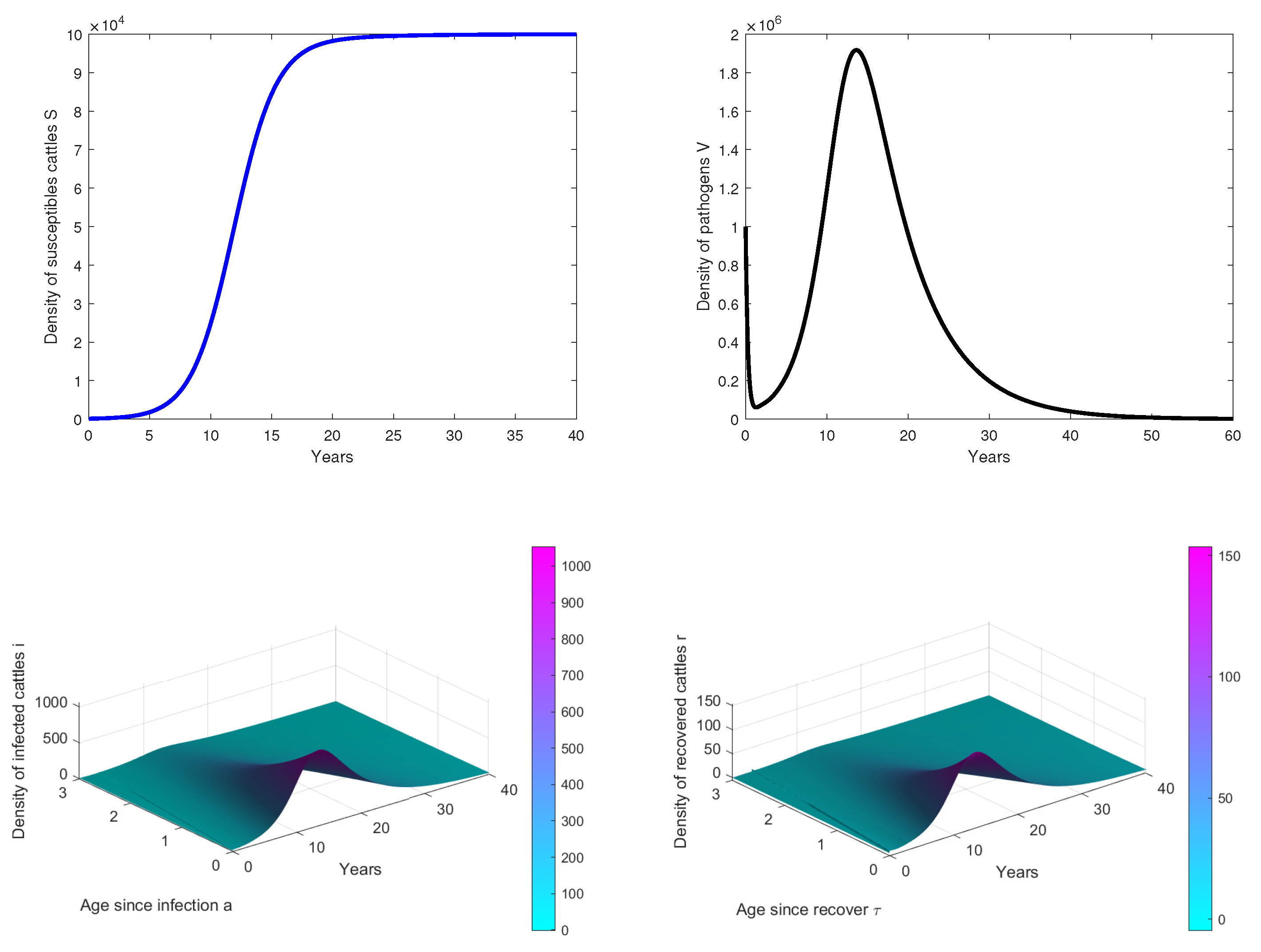
• In Figure 2, we observe that the disease dies out in the population when, ${\mathcal{R}}_0<1$. This confirms our theoretical results.
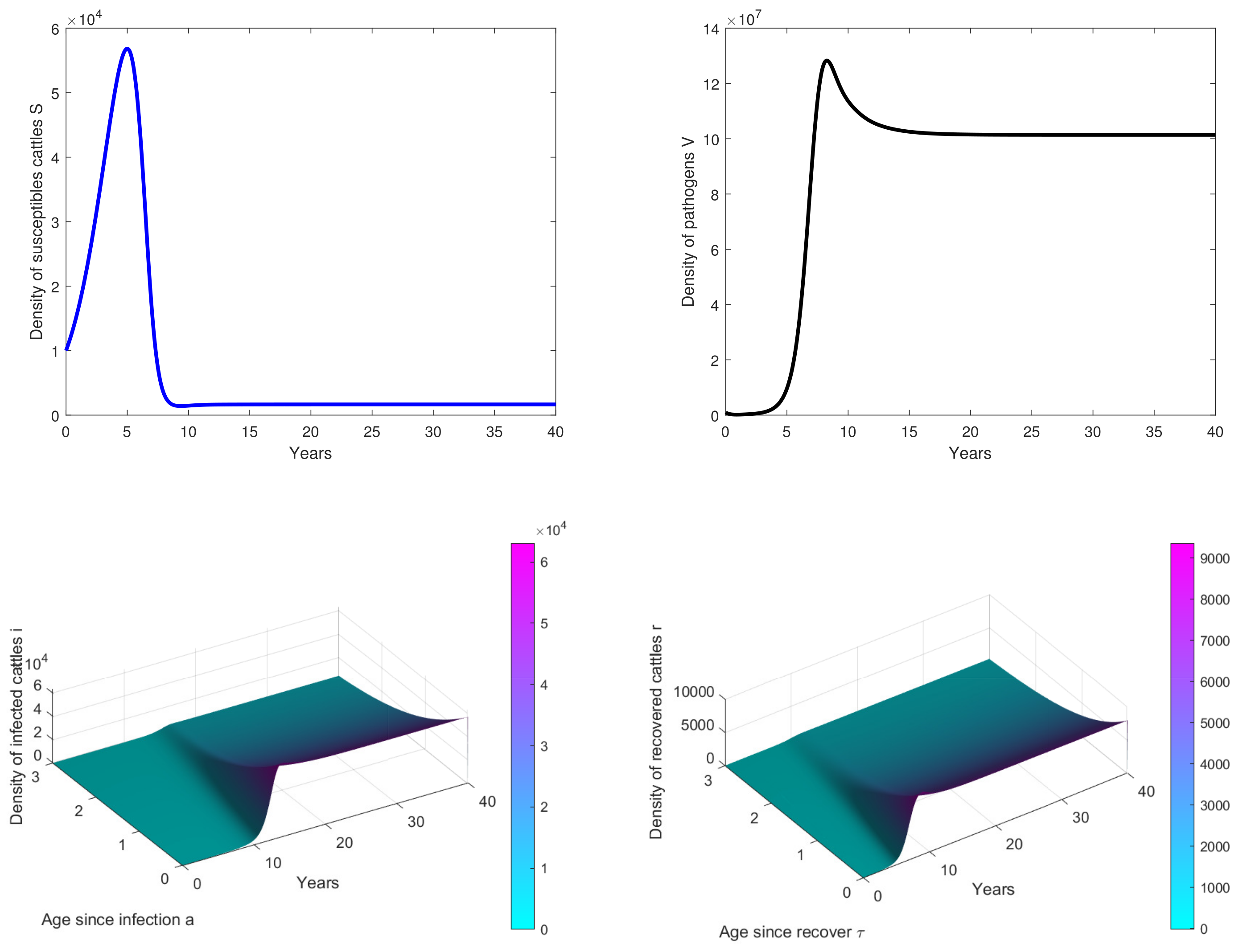
• In Figure 3, the initial dose is $V_0={10}^6$ and we observe that the peak of infection is reached about 14 years post-infection. The figure shows that the disease could persist in the population when ${\mathcal{R}}_0>1$.
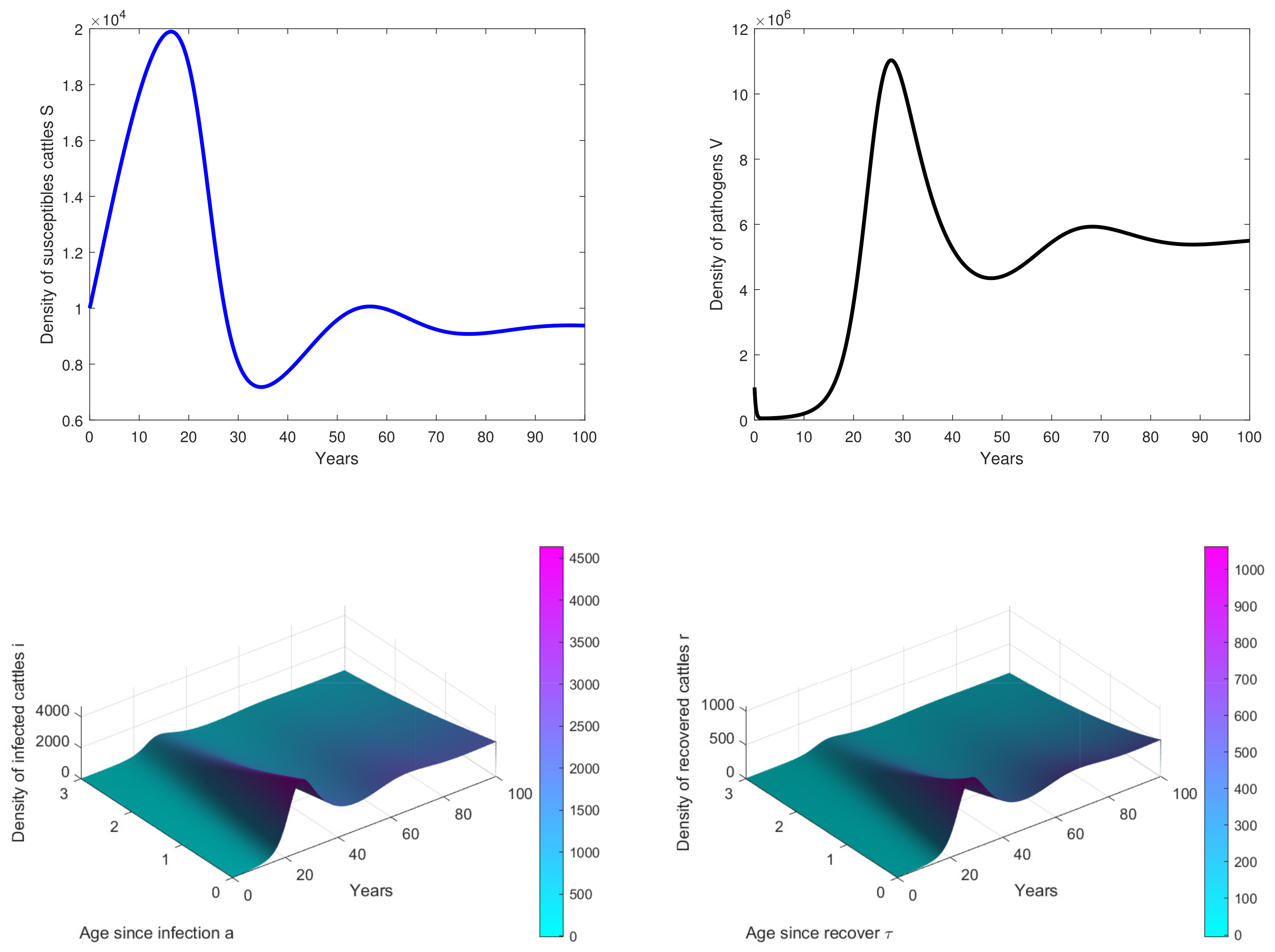
• In Figure 4, $b=0.39$, we observe that the peak of infection is reached about 10 years post-infection and there are some oscillations on the curves. This means that the birth rate of cattle significantly influences the dynamics of the disease.

6. Conclusions

In this work, we proposed a new model of brucellosis occurring in cattle populations. Because understanding the role of the adaptive immune response following exposure to brucellosis is a critical step in the development of a vaccine, our model incorporates the rate at which recovered individuals lose their immunity. We established the mathematical well-posedness results by measn of integrated semi-group theory. Furthermore, we computed the basic reproduction number and obtained an explicit form of endemic equilibrium. Finally, we performed some numerical simulations to illustrate the persistence of the disease and the epidemic evolution. The calibration of the parameters was conducted using real data retrieved from the biology of the disease.

Our study showed the possibility of several outcomes depending on the basic reproduction number ${\mathcal{R}}_0$, which led us to find the existence and stability results of the disease-free equilibrium when ${\mathcal{R}}_0<1$ (see Figure 2). Then, after obtaining an explicit form of the endemic equilibrium, we proved its local stability. The results of simulation illustrate the persistence of the disease in the population when ${\mathcal{R}}_0>1$ (see Figure 3 and Figure 4).

In Figure 4, the birth rate b has changed and we observe that there some oscillations have appeared. This means that the birth rate of the population has an influence on the disease dynamics and that by changing the values of some parameters, one could obtain periodic oscillations, suggesting that there will be periodic outbreaks of epidemics, and the disease will not be eradicated from the population [36]. Hence, it would be very interesting in our future work to study the sensitivity analysis of parameters of the model in order to identify that bifurcation parameter.

The model developed here can be further used to study the effects of vaccination on the cattle population. Indeed, if we assume that vaccination acts on the susceptible population and waning duration simultaneously, then as the population is vaccinated, the contamination rates ${\sigma }^{dir}$ and ${\sigma }^{ind}$ will decrease, since the waning duration increases. Furthermore, we note that in reality, the immune systems of individuals may be boosted through exposure to the disease. This feature is a factor considered in several existing models through the immunity clock, that is, by resetting the recovery age [37] or through the inclusion of additional internal states (within-host dynamics); see, for instance, [38,39]. This feature could be included to improve the present work.

References

- Godfroid, J. Brucellosis in livestock and wildlife: Zoonotic diseases without pandemic potential in need of innovative one health approaches. Arch. Public Health 2017, 75, 1–6. [Google Scholar] [CrossRef] [PubMed]
- Omer, M.; Skjerve, E.; Holstad, G.; Woldehiwet, Z.; Macmillan, A. Prevalence of antibodies to Brucella spp. in cattle, sheep, goats, horses and camels in the State of Eritrea; influence of husbandry systems. Epidemiol. Infect. 2000, 125, 447–453. [Google Scholar] [CrossRef] [PubMed]
- Megersa, B.; Biffa, D.; Abunna, F.; Regassa, A.; Godfroid, J.; Skjerve, E. Seroepidemiological study of livestock brucellosis in a pastoral region. Epidemiol. Infect. 2012, 140, 887–896. [Google Scholar] [CrossRef] [PubMed]
- Zhang, J.; Sun, G.Q.; Sun, X.D.; Hou, Q.; Li, M.; Huang, B.; Wang, H.; Jin, Z. Prediction and control of brucellosis transmission of dairy cattle in Zhejiang Province, China. PLoS ONE 2014, 9, e108592. [Google Scholar] [CrossRef] [PubMed]
- Rossetti, C.A.; Arenas-Gamboa, A.M.; Maurizio, E. Caprine brucellosis: A historically neglected disease with significant impact on public health. PLoS Negl. Trop. Dis. 2017, 11, e0005692. [Google Scholar] [CrossRef] [Green Version]
- Diacovich, L.; Gorvel, J.P. Bacterial manipulation of innate immunity to promote infection. Nat. Rev. Microbiol. 2010, 8, 117–128. [Google Scholar] [CrossRef]
- Dorneles, E.M.; Teixeira-Carvalho, A.; Araújo, M.S.; Sriranganathan, N.; Lage, A.P. Immune response triggered by Brucella abortus following infection or vaccination. Vaccine 2015, 33, 3659–3666. [Google Scholar] [CrossRef]
- Bang, B. Infectious Abortion in Cattle. J. Comp. Pathol. Ther. 1906, 19, 191–202. [Google Scholar] [CrossRef]
- Abatih, E.; Ron, L.; Speybroeck, N.; Williams, B.; Berkvens, D. Mathematical analysis of the transmission dynamics of brucellosis among bison. Math. Methods Appl. Sci. 2015, 38, 3818–3832. [Google Scholar] [CrossRef]
- Hou, Q.; Sun, X.; Zhang, J.; Liu, Y.; Wang, Y.; Jin, Z. Modeling the transmission dynamics of sheep brucellosis in Inner Mongolia Autonomous Region, China. Math. Biosci. 2013, 242, 51–58. [Google Scholar] [CrossRef]
- Li, M.T.; Sun, G.Q.; Zhang, W.Y.; Jin, Z. Model-based evaluation of strategies to control brucellosis in China. Int. J. Environ. Res. Public Health 2017, 14, 295. [Google Scholar] [CrossRef] [PubMed] [Green Version]
- Lolika, P.O.; Modnak, C.; Mushayabasa, S. On the dynamics of brucellosis infection in bison population with vertical transmission and culling. Math. Biosci. 2018, 305, 42–54. [Google Scholar] [CrossRef] [PubMed]
- Lolika, P.O.; Mushayabasa, S. On the role of short-term animal movements on the persistence of brucellosis. Mathematics 2018, 6, 154. [Google Scholar] [CrossRef] [Green Version]
- Nyerere, N.; Luboobi, L.S.; Mpeshe, S.C.; Shirima, G.M. Mathematical model for the infectiology of brucellosis with some control strategies. New Trends Math. Sci. 2019, 4, 387–405. [Google Scholar] [CrossRef]
- Paride, P.O.L. Modeling the Transmission Dynamics of Brucellosis. Ph.D. Thesis, University of Zimbabwe, Harare, Zimbabwe, 2019. [Google Scholar]
- Zhang, W.; Zhang, J.; Wu, Y.P.; Li, L. Dynamical analysis of the SEIB model for Brucellosis transmission to the dairy cows with immunological threshold. Complexity 2019, 2019, 6526589. [Google Scholar] [CrossRef] [Green Version]
- Hou, Q.; Sun, X.D. Modeling sheep brucellosis transmission with a multi-stage model in Changling County of Jilin Province, China. J. Appl. Math. Comput. 2016, 51, 227–244. [Google Scholar] [CrossRef]
- Lolika, P.O.; Mushayabasa, S. Dynamics and stability analysis of a brucellosis model with two discrete delays. Discret. Dyn. Nat. Soc. 2018, 2018, 6456107. [Google Scholar] [CrossRef]
- Sun, G.Q.; Li, M.T.; Zhang, J.; Zhang, W.; Pei, X.; Jin, Z. Transmission dynamics of brucellosis: Mathematical modelling and applications in China. Comput. Struct. Biotechnol. J. 2020, 18, 3843. [Google Scholar] [CrossRef]
- Tumwiine, J.; Robert, G. A mathematical model for treatment of bovine brucellosis in cattle population. J. Math. Model. 2017, 5, 137–152. [Google Scholar]
- Lolika, P.O.; Mushayabasa, S.; Bhunu, C.P.; Modnak, C.; Wang, J. Modeling and analyzing the effects of seasonality on brucellosis infection. Chaos Solitons Fractals 2017, 104, 338–349. [Google Scholar] [CrossRef]
- Yang, J.; Xu, R.; Li, J. Threshold dynamics of an age–space structured brucellosis disease model with Neumann boundary condition. Nonlinear Anal. Real World Appl. 2019, 50, 192–217. [Google Scholar] [CrossRef]
- Yang, J.; Xu, R.; Sun, H. Dynamics of a seasonal brucellosis disease model with nonlocal transmission and spatial diffusion. Commun. Nonlinear Sci. Numer. Simul. 2021, 94, 105551. [Google Scholar] [CrossRef]
- Ainseba, B.; Benosman, C.; Magal, P. A model for ovine brucellosis incorporating direct and indirect transmission. J. Biol. Dyn. 2010, 4, 2–11. [Google Scholar] [CrossRef] [PubMed]
- Nannyonga, B.; Mwanga, G.; Luboobi, L. An optimal control problem for ovine brucellosis with culling. J. Biol. Dyn. 2015, 9, 198–214. [Google Scholar] [CrossRef] [PubMed] [Green Version]
- Ganiere, J.P. La brucellose animale. Ecoles Nationales Vétérinaires Françaises Merial, 2004; 1–47. [Google Scholar]
- Richard, Q.; Choisy, M.; Lefèvre, T.; Djidjou-Demasse, R. Human-vector malaria transmission model structured by age, time since infection and waning immunity. Nonlinear Anal. Real World Appl. 2022, 63, 103393. [Google Scholar] [CrossRef]
- Magal, P.; Seydi, O.; Wang, F.B. Monotone abstract non-densely defined Cauchy problems applied to age structured population dynamic models. J. Math. Anal. Appl. 2019, 479, 450–481. [Google Scholar] [CrossRef] [Green Version]
- Martcheva, M.; Thieme, H.R. Progression age enhanced backward bifurcation in an epidemic model with super-infection. J. Math. Biol. 2003, 46, 385–424. [Google Scholar] [CrossRef]
- Roth, F.; Zinsstag, J.; Orkhon, D.; Chimed-Ochir, G.; Hutton, G.; Cosivi, O.; Carrin, G.; Otte, J. Human health benefits from livestock vaccination for brucellosis: Case study. Bull. World Health Organ. 2003, 81, 867–876. [Google Scholar]
- Magal, P.; McCluskey, C.; Webb, G. Lyapunov functional and global asymptotic stability for an infection-age model. Appl. Anal. 2010, 89, 1109–1140. [Google Scholar] [CrossRef]
- Kenne, C.; Dorville, R.; Mophou, G.; Zongo, P. An Age-Structured Model for Tilapia Lake Virus Transmission in Freshwater with Vertical and Horizontal Transmission. Bull. Math. Biol. 2021, 83, 1–35. [Google Scholar] [CrossRef]
- Jiao, J.; Yang, J.; Yang, X. The dairy cattle brucellosis and prevention and control (Nainiu bulujunbing jiqi fangkong). Anim. Husb. Feed. Sci. 2009, 30, 170–171. [Google Scholar]
- Dobson, A.; Meagher, M. The population dynamics of brucellosis in the Yellowstone National Park. Ecology 1996, 77, 1026–1036. [Google Scholar] [CrossRef]
- Sun, T.; Wu, Z.; Pang, X. Prevention measures and countermeasures on brucellosis in Inner Mongolia. Neimenggu Prev. Med. 2000, 1, 136–139. [Google Scholar]
- Blyuss, K.B.; Kyrychko, Y.N. Stability and bifurcations in an epidemic model with varying immunity period. Bull. Math. Biol. 2010, 72, 490–505. [Google Scholar] [CrossRef] [Green Version]
- Okuwa, K.; Inaba, H.; Kuniya, T. An age-structured epidemic model with boosting and waning of immune status. Math. Biosci. Eng. 2021, 18, 5707–5736. [Google Scholar] [CrossRef]
- Gandolfi, A.; Pugliese, A.; Sinisgalli, C. Epidemic dynamics and host immune response: A nested approach. J. Math. Biol. 2015, 70, 399–435. [Google Scholar] [CrossRef] [Green Version]
- Gulbudak, H.; Cannataro, V.L.; Tuncer, N.; Martcheva, M. Vector-borne pathogen and host evolution in a structured immuno-epidemiological system. Bull. Math. Biol. 2017, 79, 325–355. [Google Scholar] [CrossRef]