A Time-Delayed Deterministic Model for the Spread of COVID-19 with Calibration on a Real Dataset

Abstract

During the evolution of the COVID-19 pandemic, each country has adopted different control measures to contrast the epidemic’s diffusion. Restrictions to mobility, public transport, and social life in general have been actuated to contain the spread of the pandemic. In this paper, we consider the deterministic SIRD model with delays proposed by Calleri et al., which is improved by adding the vaccinated compartment V (SIRDV model) and considering a time-dependent contact frequency. The three delays take into account the incubation time of the disease, the healing time, and the death time. The aim of this work is to study the effect of the vaccination campaigns in Great Britain (GBR) and Israel (ISR) during the pandemic period. The different restriction periods are included by fitting the contact frequency on real datasets as a piecewise constant function. As expected, the vaccination campaign reduces the amount of deaths and infected people. Furthermore, for the different levels of restriction policy, we find specific values of the contact frequency that can be used to predict the trend of the pandemic.

1. Introduction

COVID-19, the acronym for Coronavirus Disease 2019, is a infectious respiratory disease caused by the virus called SARS-CoV-2 belonging to the coronavirus family. It has spread rapidly and has taken millions of lives worldwide since the end of 2019 [1].

Epidemic models can be devised with the aim to predict the pandemic’s evolution. They represent a class of mathematical models that are used not only to study epidemics properly, but also to predict social phenomena or the behavior of biological systems and, for these reasons, they have been a branch of interest in applied mathematics for several years. Epidemic models can help governments decide on the best restriction policy to adopt so that the virus’ spread can be contained in a better way [2,3]. The crucial point consists in determining suitable parameters of such models that are able to represent and predict accurately the behavior of the illness.

Regarding the COVID-19 pandemic, many mathematical models have been proposed. Epidemic models based on ordinary differential equations have been introduced in [2,4,5]. Stochastic models have been proposed in [6,7]. For models based on stochastic differential equations, see, e.g., [8,9]. A model based on an operatorial approach, as in quantum mechanics, can be found in [10]. A continuous space-time non-linear probabilistic model has been proposed in [11], where the interpretation is given in analogy with quantum mechanics.

In [7] a deterministic model based on differential equations with time delays has been devised, although it was introduced only to validate the stochastic one and no applications have been provided by using such a model. In [12,13], mathematical models with only a delay regarding the incubation time are presented. In the present work, we consider a compartmental model consisting in dividing the population in four categories: susceptible S, infected I, recovered R, and dead D (SIRD model). The transitions between classes are governed by a system of differential equations with delays. The adopted model considers three time delays: the incubation time, the healing time, and the death time. The use of time delays allows the inclusion of characteristics of the disease under consideration, such as incubation, and also possible delays due to data communication and recording. Moreover, we provide an application of the model mentioned above to the cases of the COVID-19 spread in Great Britain (GBR) and Israel (ISR). The parameters are extracted from real data collected in [14] by a fitting procedure, and a comparison with the policy measures to prevent the pandemic diffusion is made. Furthermore, the effect of vaccination is a key point for the pandemic’s evolution, and therefore, several studies are carried out (see, e.g., [15]). For this reason, we include, in the examined SIRD model, the further category of vaccinated people V, for which time evolution is provided by data, thus defining a SIRDV model. In this way, we include the effect of vaccination in the examined model for the countries under investigation to predict different scenarios depending on whether it is considered or not.

The plan of the paper is as follows. In Section 2, the SIRD and SIRDV mathematical models are introduced; in Section 3, the numerical approach to simulate the previous models is presented and applied for a specific analysis of the single country under consideration. In particular, in Section 3.2, we perform a data-fitting for ISR to obtain the SIRDV model parameters, and we also obtain numerical simulations, and in Section 3.3, the same analysis is completed for GBR; in Section 4, we perform a comparison between the parameters of the model found for the two countries and we show the results of the simulations. Furthermore, we use two statistical tests, i.e., ANOVA and Kruskal–Wallis, to confirm the dependence between the values of the contact frequency and the containment measures.

2. Mathematical Model

The simplest epidemic model is the well-known SIR model [16,17]. It arises as a deterministic model which consists of a system of ordinary differential equations describing the time evolution of three classes: susceptible (S), infected (I) and recovered (R). If the class of dead (D) people is also considered, the model takes the name of SIRD. Since COVID-19 has a relevant incubation period [18] and an identifiable period from infection to recovery [19], in [7], a SIRD model with time delays has been proposed as follows.

We suppose that the disease has an incubation time ${\tau }_1$, a healing time ${\tau }_2$, and a death time ${\tau }_3$. Let $t\ge {\tau }_1$. At time $t+\Delta t$, the number of the susceptibles, $S(t+\Delta t)$, decreases because some of the susceptibles at time t, $S\left(t\right)$, become infected. The number of the susceptibles that become infected over the time frame $\Delta t$ is proportional to $S\left(t\right)$ times the fraction of infected people at the previous time $t-{\tau }_1$, $I(t-{\tau }_1)/N$, due to the incubation time, where N is the entire population size. The proportionality factor is the contact frequency $\beta$ of a susceptible individual that leads to an infection. Moreover, for $t<{\tau }_1$, we suppose that new infections do not occur over the time frame $\Delta t$ and, to include this assumption, we multiply for $H(t-{\tau }_1)$, where $H(·)$ is the Heaviside step function. Therefore, we have:

$${\displaystyle \frac{S(t+\Delta t)-S\left(t\right)}{\Delta t}}=-\beta S\left(t\right){\displaystyle \frac{I(t-{\tau }_1)}{N}}H(t-{\tau }_1),$$

(1)

and for $\Delta t$ going to 0, we obtain:

$$\dot{S}\left(t\right)=-\beta S\left(t\right){\displaystyle \frac{I(t-{\tau }_1)}{N}}H(t-{\tau }_1).$$

Let $\alpha$ be the mortality rate, which is defined as the infection–fatality ratio (IFR), i.e., the ratio between the number of deaths from disease and the number of infected individuals. To describe the recovering mechanism, we assume that the increase of recovered people at time t is due to the decrease of susceptible people at time $t-{\tau }_2$ multiplied by $1-\alpha$, that is:

$$\dot{R}\left(t\right)=-(1-\alpha )\dot{S}(t-{\tau }_2).$$

In a similar way, we model the death mechanism, obtaining:

$$\dot{D}\left(t\right)=-\alpha \dot{S}(t-{\tau }_3).$$

Finally, the variation of infected is obtained by the sum of three contributions: the first one is the opposite of the variation of the susceptibles; the second one is the opposite of the variation of those who have recovered, and the last one is the opposite of the variation of the those who have died. Indeed, an individual who becomes infected leaves the S class and joins the I class; an infected individual that recovers passes from the I class to the R class; an infected individual that dies passes from the I class to the D class.

From these considerations, the following equations of the SIRD deterministic model are proposed:

$$\left\{\begin{array}{c}\dot{S}\left(t\right)=-\beta S\left(t\right){\displaystyle \frac{I(t-{\tau }_1)}{N}}H(t-{\tau }_1),\hfill \\ \dot{I}\left(t\right)=\beta S\left(t\right){\displaystyle \frac{I(t-{\tau }_1)}{N}}H(t-{\tau }_1)+(1-\alpha )\dot{S}(t-{\tau }_2)+\alpha \dot{S}(t-{\tau }_3),\hfill \\ \dot{R}\left(t\right)=-(1-\alpha )\dot{S}(t-{\tau }_2),\hfill \\ \dot{D}\left(t\right)=-\alpha \dot{S}(t-{\tau }_3).\hfill \end{array}\right.$$

(2)

This model falls into the class of differential delay equations with multiple time lags. The theory of time-delayed differential equations is an active research topic. The interested reader can refer to [20] for an overview. Regarding the specific problem of this paper, a qualitative theoretical analysis is not provided. Some analytic results, valid in a more general class, can be found in [21].

By substituting the expression of $\dot{S}$ given by the first equation of the system (2) in the remaining equations of the system, the latter can be rewritten as:

$$\left\{\begin{array}{c}\dot{S}\left(t\right)=-\beta S\left(t\right){\displaystyle \frac{I(t-{\tau }_1)}{N}}H(t-{\tau }_1),\hfill \\ \dot{I}\left(t\right)=\beta S\left(t\right){\displaystyle \frac{I(t-{\tau }_1)}{N}}H(t-{\tau }_1)+\hfill \\ -(1-\alpha )[\beta S(t-{\tau }_2){\displaystyle \frac{I(t-{\tau }_1-{\tau }_2)}{N}}H(t-{\tau }_1-{\tau }_2)]\hfill \\ -\alpha \left[\beta S(t-{\tau }_3){\displaystyle \frac{I(t-{\tau }_1-{\tau }_3)}{N}}H(t-{\tau }_1-{\tau }_3)\right],\hfill \\ \dot{R}\left(t\right)=(1-\alpha )\left[\beta S(t-{\tau }_2){\displaystyle \frac{I(t-{\tau }_1-{\tau }_2)}{N}}H(t-{\tau }_1-{\tau }_2)\right],\hfill \\ \dot{D}\left(t\right)=\alpha \left[\beta S(t-{\tau }_3){\displaystyle \frac{I(t-{\tau }_1-{\tau }_3)}{N}}H(t-{\tau }_1-{\tau }_3)\right].\hfill \end{array}\right.$$

(3)

Moreover, to include the effect of the vaccination campaign, we improve the model by introducing the variable V, which represents the total number of cumulative vaccinated people. The aim of the vaccination campaign is to decrease the number of susceptible individuals and to weaken the pandemic. Let us consider Equation (1); we subtract at the right-hand side the variation of vaccinated people over the time frame $\Delta t$, that is:

$${\displaystyle \frac{S(t+\Delta t)-S\left(t\right)}{\Delta t}}=-\beta S\left(t\right){\displaystyle \frac{I(t-{\tau }_1)}{N}}H(t-{\tau }_1)-\frac{V(t+\Delta t)-V\left(t\right)}{\Delta t},$$

and for $\Delta t$ going to 0, we obtain:

$$\dot{S}\left(t\right)=-\beta S\left(t\right){\displaystyle \frac{I(t-{\tau }_1)}{N}}H(t-{\tau }_1)-\dot{V}\left(t\right).$$

We do not provide a model for $V\left(t\right)$ because, in the applications of the next sections, we obtain its values from data. Another improvement of the model consists in considering $\beta$ as a function of time, whose expression will be explained below. Therefore, we propose the following SIRDV model:

$$\left\{\begin{array}{c}\dot{S}\left(t\right)=-\beta \left(t\right)S\left(t\right){\displaystyle \frac{I(t-{\tau }_1)}{N}}H(t-{\tau }_1)-\dot{V}\left(t\right),\hfill \\ \dot{I}\left(t\right)=\beta \left(t\right)S\left(t\right){\displaystyle \frac{I(t-{\tau }_1)}{N}}H(t-{\tau }_1)\hfill \\ -(1-\alpha )[\beta (t-{\tau }_2)S(t-{\tau }_2){\displaystyle \frac{I(t-{\tau }_1-{\tau }_2)}{N}}H(t-{\tau }_1-{\tau }_2)]\hfill \\ -\alpha \left[\beta (t-{\tau }_3)S(t-{\tau }_3){\displaystyle \frac{I(t-{\tau }_1-{\tau }_3)}{N}}H(t-{\tau }_1-{\tau }_3)\right],\hfill \\ \dot{R}\left(t\right)=(1-\alpha )\left[\beta (t-{\tau }_2)S(t-{\tau }_2){\displaystyle \frac{I(t-{\tau }_1-{\tau }_2)}{N}}H(t-{\tau }_1-{\tau }_2)\right],\hfill \\ \dot{D}\left(t\right)=\alpha \left[\beta (t-{\tau }_3)S(t-{\tau }_3){\displaystyle \frac{I(t-{\tau }_1-{\tau }_3)}{N}}H(t-{\tau }_1-{\tau }_3)\right].\hfill \end{array}\right.$$

(4)

In (4), the function $\beta \left(t\right)$ is modeled as a piecewise constant function that depends on the more or less restrictive policies along all the days considered, that is:

$$\beta \left(t\right)=\left\{\begin{array}{cc}{\beta }_0,T_{min}\le t\le {\tilde{t}}_0,\hfill & \\ {\beta }_1,{\tilde{t}}_0<t\le {\tilde{t}}_1,\hfill & \\ ⋮⋮\hfill & \\ {\beta }_i,{\tilde{t}}_{i-1}<t\le {\tilde{t}}_i,\hfill & \\ ⋮⋮\hfill & \\ {\beta }_n,{\tilde{t}}_{n-1}<t\le T_{max},\hfill \end{array}\right.$$

(5)

where ${\beta }_0,{\beta }_1,\cdots ,{\beta }_i,\cdots ,{\beta }_n$, and ${\tilde{t}}_0,{\tilde{t}}_1,\cdots ,{\tilde{t}}_i,\cdots ,{\tilde{t}}_{n-1}$ are parameters to be estimated, and $T_{min}$ and $T_{max}$ correspond to the first and last day of the investigated period, respectively. We note that $0\le \beta \left(t\right)\le 1$, and if $\beta \left(t\right)\approx 1$, it means that the contact frequency is greater and there are few restrictive measures; on the contrary, if $\beta \left(t\right)\approx 0$, it implies a lockdown period.

Upon these considerations, we would like to find the parameters needed in the proposed model by a non-linear optimization procedure based on the Nelder–Mead method, implemented in MATLAB [22]. Some convergence properties of the method in low dimensions can be found in [23]. The target is the minimization of the functional:

$$J=\parallel I-I_d\parallel +\parallel R-R_d\parallel +\parallel D-D_d\parallel ,$$

where $\parallel ·\parallel$ is the 2-norm, I, R, and D are the numerical solutions of the model, and $I_d$, $R_d$, and $D_d$ are the same quantities given by official data for GBR and ISR, i.e., the actual number of infections, the cumulative number of recoveries, and the cumulative number of deaths.

3. Simulations and Results

In this section, the numerical approach is presented and the results of the simulations are reported and commented on. We analyze the COVID-19 epidemic’s behavior in two different countries: ISR and GBR. The time interval starts from the onset of the pandemic and includes several waves of infection. The dataset used for both countries has been taken from [14].

3.1. Numerical Approach

In order to find numerical solutions of the system (4), we adopt a first-order finite differences scheme. Let us fix a temporal grid $T_{min}=t_0<t_1<\dots <t_M=T_{max}$ of constant time step $\Delta t$ small enough to guarantee numerical stability. We introduce the numerical approximations $S_k\approx S\left(t_k\right),$ $I_k\approx I\left(t_k\right),$ $R_k\approx R\left(t_k\right),$ $D_k\approx D\left(t_k\right),$ $V_k\approx V\left(t_k\right)$, and ${\beta }_k\approx \beta \left(t_k\right)$ for $k=0,1,\dots ,M$, and we discretize the system (4) as follows:

$$\begin{array}{cc}\hfill S_{k+1}=& S_k-\frac{\Delta t}{N}{\beta }_k{S}_k{I}_{k_1}H(t_k-{\tau }_1)-(V_{k+1}-V_k),\hfill \\ \hfill I_{k+1}=& I_k+\frac{\Delta t}{N}{\beta }_k{S}_k{I}_{k_1}H(t_k-{\tau }_1)\hfill \\ \hfill & -(1-\alpha )\frac{\Delta t}{N}{\beta }_{k_2}{S}_{k_2}{I}_{k_{12}}H(t_k-{\tau }_1-{\tau }_2)\hfill \\ \hfill & -\alpha \frac{\Delta t}{N}{\beta }_{k_3}{S}_{k_3}{I}_{k_{13}}H(t_k-{\tau }_1-{\tau }_3),\hfill \\ \hfill R_{k+1}=& R_k+\frac{\Delta t}{N}(1-\alpha ){\beta }_{k_2}{S}_{k_2}{I}_{k_{12}}H(t_k-{\tau }_1-{\tau }_2),\hfill \\ \hfill D_{k+1}=& D_k+\alpha \frac{\Delta t}{N}{\beta }_{k_3}{S}_{k_3}{I}_{k_{13}}H(t_k-{\tau }_1-{\tau }_3),\hfill \end{array}$$

where the indexes $k_1$, $k_2$, $k_3$, $k_{12}$, and $k_{13}$ are given by:

$$k_j=max\left\{0,⌊\frac{t_k-{\tau }_j}{\Delta t}⌋\right\}j=1,2,3,$$

$$k_{1m}=max\left\{0,⌊\frac{t_k-{\tau }_1-{\tau }_m}{\Delta t}⌋\right\}m=2,3,$$

with $⌊·⌋$ being the floor function.

3.2. ISR Analysis

We consider the data in the temporal range that goes from the day of detection of the first infection, i.e., 21 February 2020, until 30 April 2021. For each variable, the dataset contains a value for each of the 435 days, but for the numerical solutions of the system (4), a temporal grid with a smaller step size $\Delta t$ needs to be fixed. For this reason, we use the spline interpolation of data to have a match with different vector lengths.

In the dataset, the number of vaccines is reported, that is, the cumulative number of administrated doses. In the proposed model, the number of vaccinated people is needed. Therefore, in order to estimate the number of vaccinated people, we divide the number of doses by 1.7, considering the number of people that have received two doses of a vaccine.

In

Table 1. Parameters adopted for the simulation in the case of ISR.

Parameter	Value
$\alpha$	0.0085
${\tau }_1$	5.5 d
${\tau }_2$	17 d
${\tau }_3$	20 d

, the adopted values of $\alpha , {\tau }_1, {\tau }_2, {\tau }_3$ are reported. The value of $\alpha$ is estimated by dividing the number of deaths by the number of infected people and averaging the result.

In order to have a more precise agreement between our model and the data, we divide the investigated period of time into several periods. In this case, we select four periods: the first one from day 1 until day 98, the second one from day 99 until day 200, the third one from day 201 until day 300, and the fourth one from day 301 until day 435. Each period is associated with an epidemic wave in which we recognize a proper number of phases of diffusion depending on the different restriction policies adopted. In particular, stronger restrictions correspond to lower values of $\beta \left(t\right)$, and vice versa. More precisely, we consider two phases for the first and third wave, and three phases for the second and fourth one.

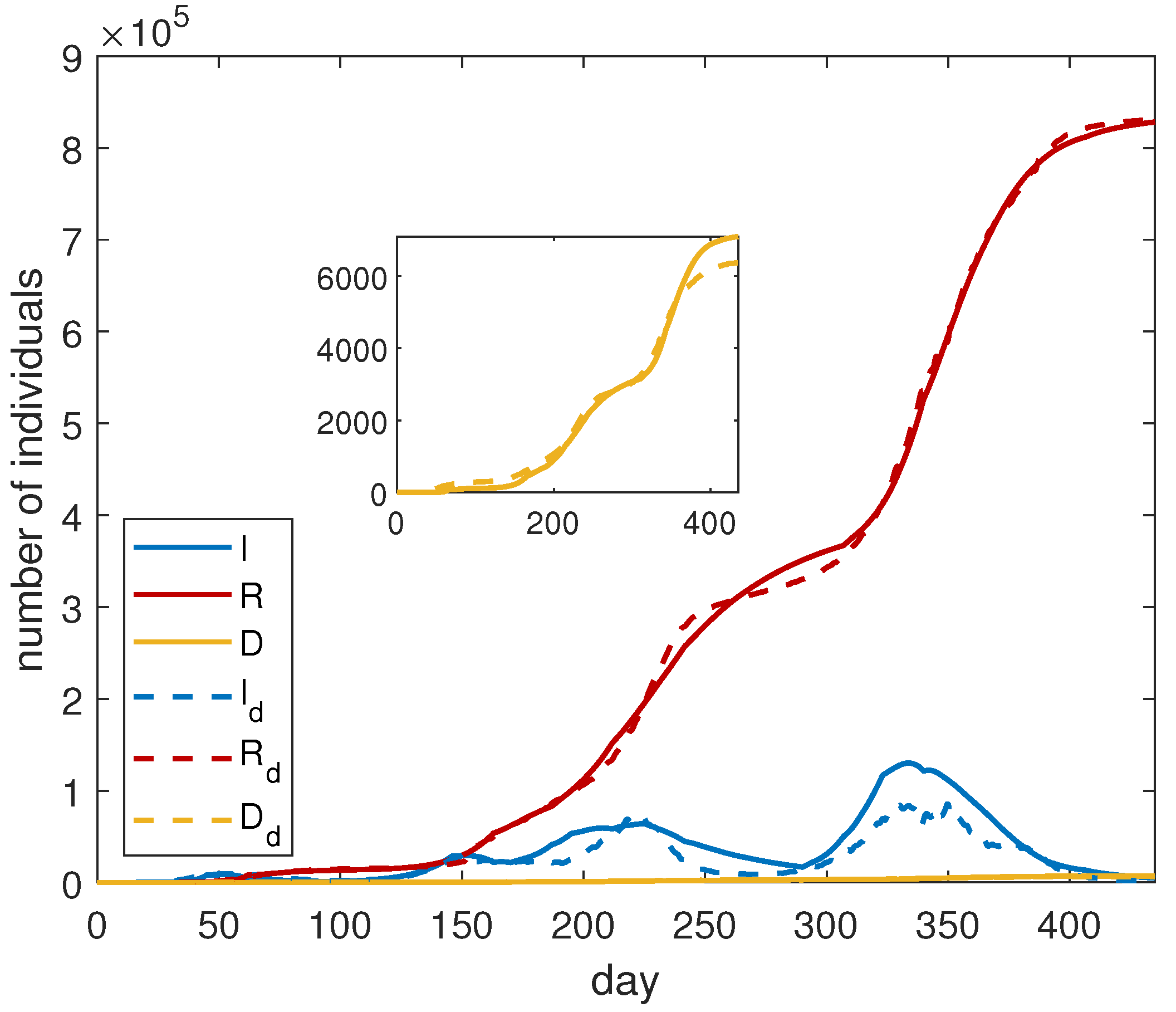
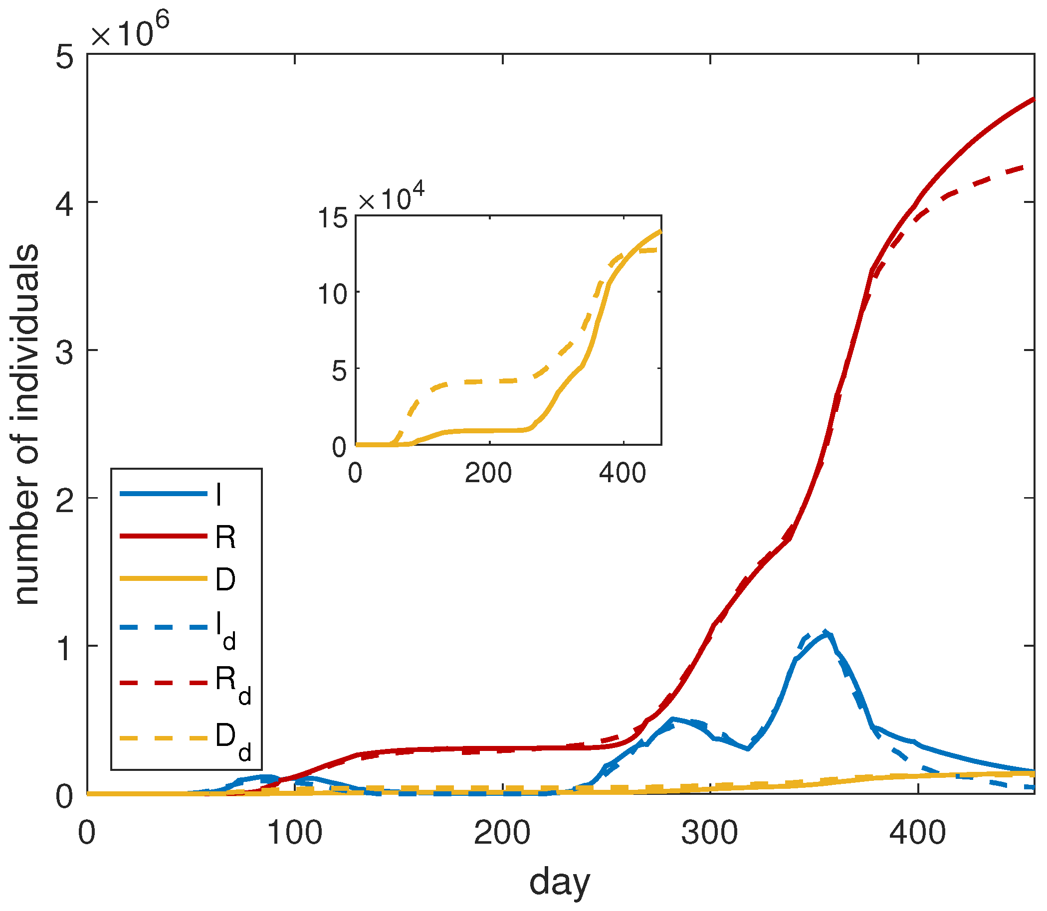
For the optimization procedure, we adopt the following strategy: we find the fitting parameters in each period corresponding to a single epidemic wave. Then, the data are merged and the optimization is applied to the entire dataset. The overall results are shown in Figure 1, and the corresponding fitting parameters are reported in

Table 2. Fitting parameters for the SIRDV model (4) applied to ISR.

Estimated Parameters
$\mathit{\beta }$	Value	t	Value
${\beta }_0$	0.72152 d${}^{-1}$	${\tilde{t}}_0$	45.04975 d
${\beta }_1$	0.026274 d${}^{-1}$	${\tilde{t}}_1$	98.01835 d
${\beta }_2$	0.14467 d${}^{-1}$	${\tilde{t}}_2$	146.0086 d
${\beta }_3$	0.046757 d${}^{-1}$	${\tilde{t}}_3$	170.0053 d
${\beta }_4$	0.0969 d${}^{-1}$	${\tilde{t}}_4$	195.0024 d
${\beta }_5$	0.0645 d${}^{-1}$	${\tilde{t}}_5$	224.9946 d
${\beta }_6$	0.0444 d${}^{-1}$	${\tilde{t}}_6$	289.993 d
${\beta }_7$	0.13793 d${}^{-1}$	${\tilde{t}}_7$	323.0012 d
${\beta }_8$	0.080843 d${}^{-1}$	${\tilde{t}}_8$	389.9505 d
${\beta }_9$	0.12619 d${}^{-1}$

. We observe that the proposed model is able to keep the several waves of infection. This is primarily due to the fine modeling of $\beta \left(t\right)$. We notice a good agreement between the simulated curves and the data.

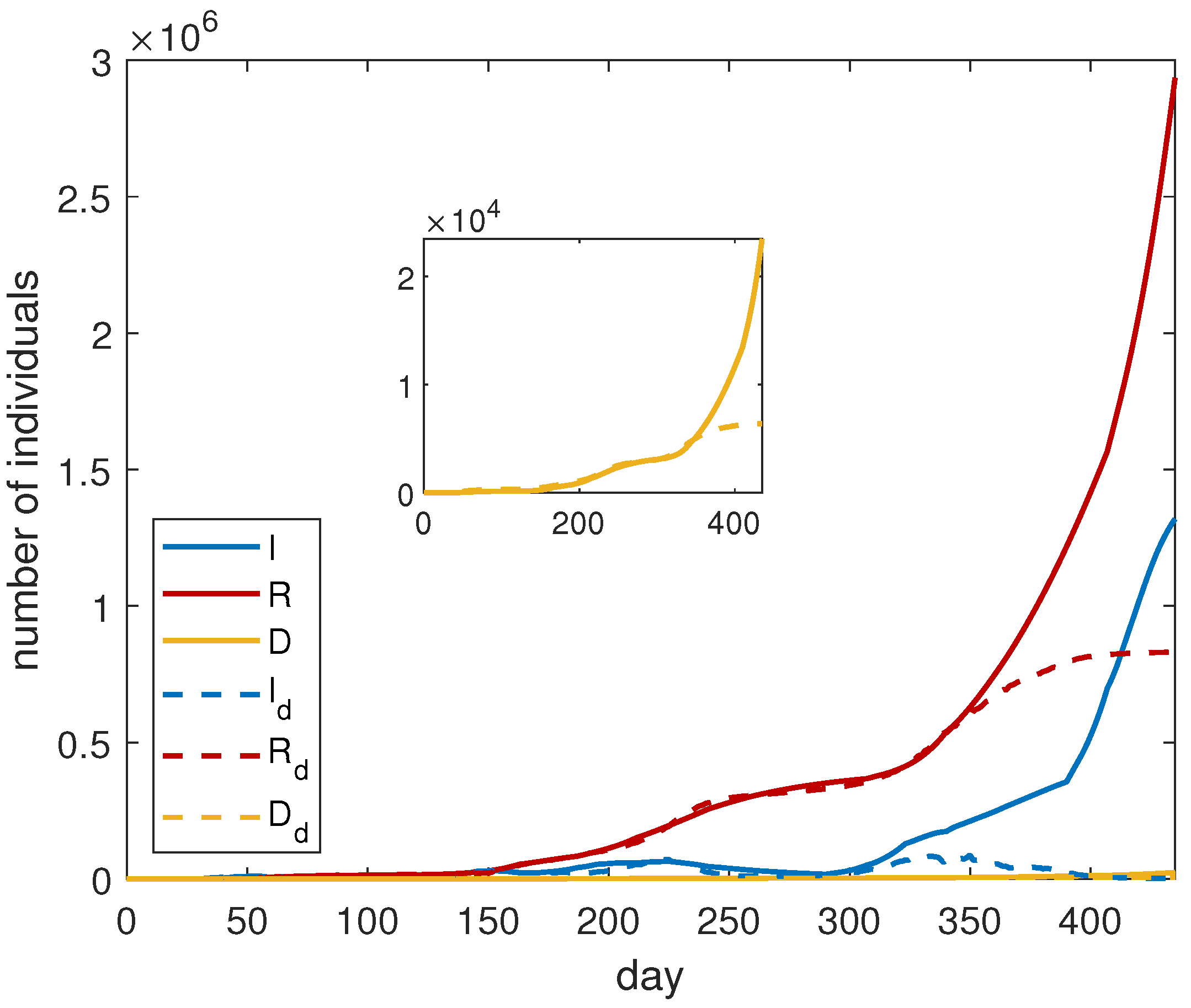
In order to quantify the importance of vaccines, we compare the results with the solutions of system (3), adopting the same parameters of Table 2. The obtained results are shown in Figure 2. We observe that, without vaccines, the number of infected and dead people would increase exponentially. This is due to a quite high value of the contact frequency in the last intervals of time. We deduce that an increasing number of vaccinated people allows the governments to adopt a less-restrictive policy, remarking on, in this way, the importance of the vaccination campaign.

Since the crucial point for containing the spread of the disease consists in preventing new cases, some parameters can be defined to provide insight into the state of the pandemic. One of the parameters used for that purpose is the basic reproduction number $R_0$. It represents the average number of infections generated by a single infected individual if all the individuals are susceptible. In the case of an ongoing outbreak, it is defined as the effective reproduction number $R_t$, which is the average number of new infections generated by a single infected individual at time t, considering the part of the population that represents susceptible individuals. Following [24], we calculate the $R_t$ numerically by using the results of our simulations. In particular, from the first two equations of system (2) we obtain:

$$\frac{\mathrm{d}I}{\mathrm{d}S}=-1+\frac{1}{R_t\left(t\right)}.$$

It can be discretized in an interval $(t_i,t_{i+1})$, where $R_t$ is constant, obtaining:

$$R_t\left(t\right)=\frac{1}{\frac{{\Delta }_{i}I}{{\Delta }_{i}S}+1},\forall t\in (t_i,t_{i+1}),$$

where ${\Delta }_{i}I=I\left(t_{i+1}\right)-I\left(t_i\right)$ and ${\Delta }_{i}S=S\left(t_{i+1}\right)-S\left(t_i\right)$.

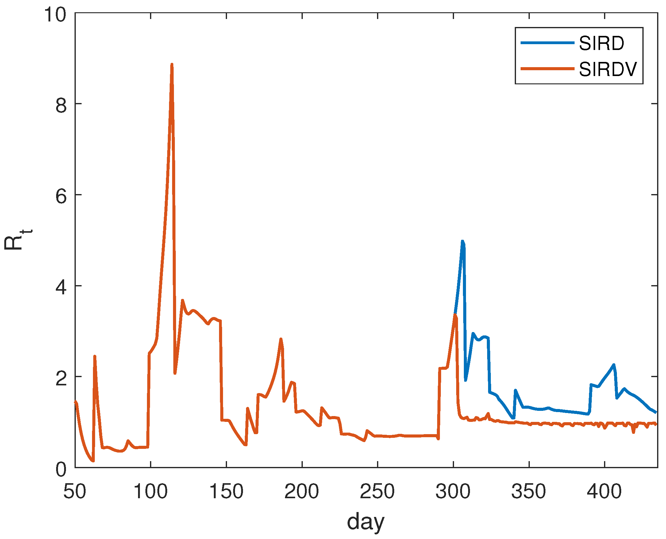
In the case of ISR, we show the results of the numerical evaluation of $R_t$ in Figure 3. It is calculated daily. The plotted time interval starts from 11 April 2020, that is, 50 days following the detection of the first infection. This choice is due to the fact that, in the first period, the curves are flat, leading to an inaccurate evaluation of $R_t$. We observe that, after approximately 300 days, the effect of vaccination becomes relevant in order to reduce the $R_t$ values.

3.3. GBR Analysis

We consider the data in the temporal range that goes from the day of the detection of the first infection, i.e., 31 January 2020, until 30 April 2021. As in the case of ISR, we perform the spline interpolation of the data.

Similar to ISR, to estimate the number of people vaccinated, we divide the number of doses provided by the data by 1.45, taking into account the number of people that have received two doses of a vaccine. Since GBR does not report the number of people who have recovered from COVID-19, to obtain the missing data, we adopt the following formula:

$$R_d\left(t\right)=(1-\alpha )I_d(t-{\tau }_1-{\tau }_2),$$

where $R_d\left(t\right)$ represents the number of recovered people at the time t, $\alpha$ represents the mortality rate, and $I_d$ represents the number of infected people at previous time $t-{\tau }_1-{\tau }_2$.

In

Table 3. Parameters adopted for the simulation in the case of GBR.

Parameter	Value
$\alpha$	0.0289
${\tau }_1$	5.5 d
${\tau }_2$	20 d
${\tau }_3$	20 d

, we report the adopted values of $\alpha , {\tau }_1, {\tau }_2, {\tau }_3$ in the simulation. In this case, the value of $\alpha$ is estimated by dividing the number of total deaths by the number of total infected people.

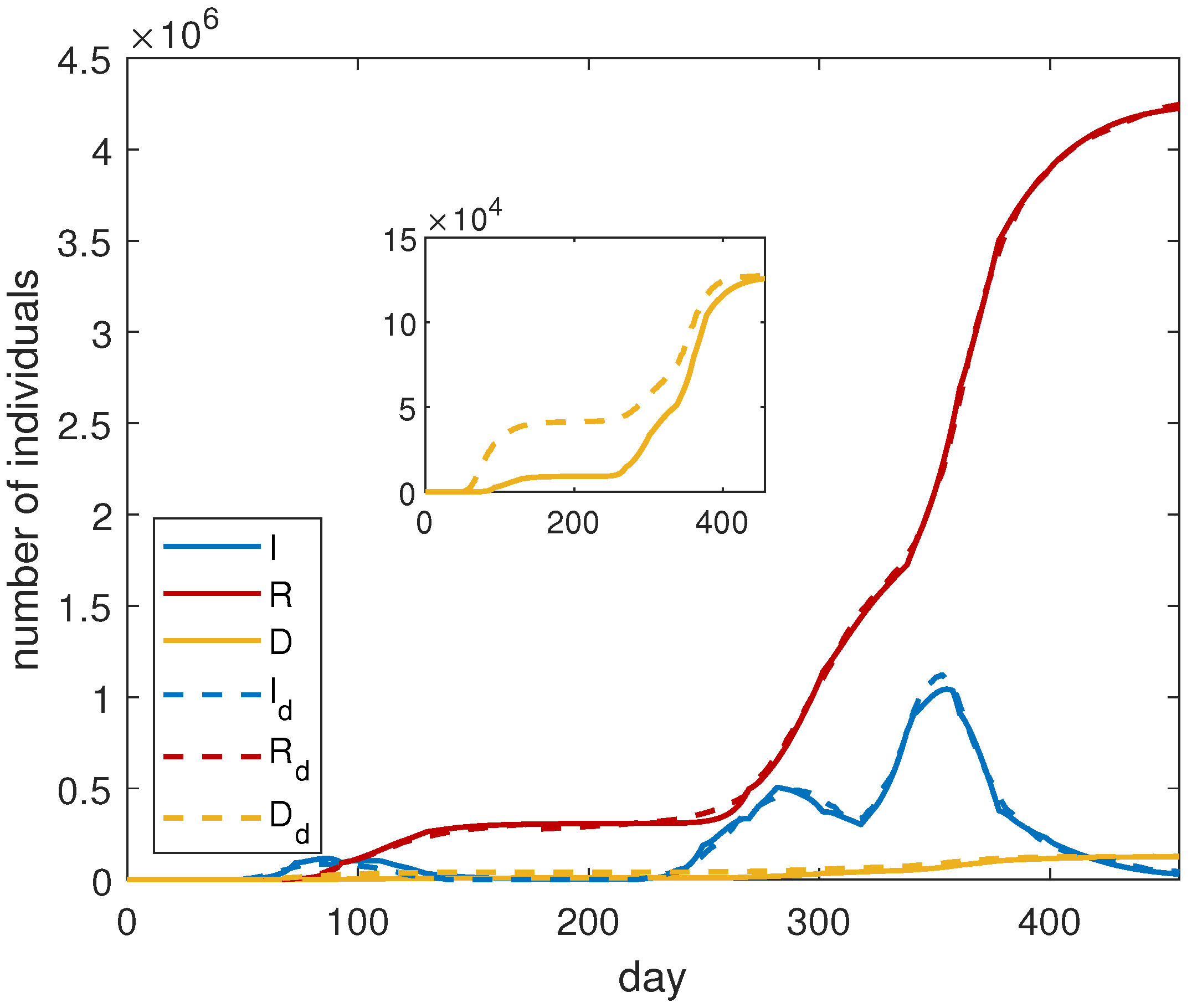
As we have done for ISR, to have a more precise agreement between our model and the data, we split the investigated period of time into three parts: the first one, from day 1 until day 221; the second one, from day 222 until day 318; the third one, from day 319 until day 456. Each period is associated with a wave of infection, in which we recognize a proper number of phases of diffusion. More precisely, we consider three phases for the first and the second wave and four phases for the third one. After finding, in each period, the best parameters thanks to the optimization, the data are merged again and the optimization is applied to the entire dataset. The results are shown in Figure 4, and the final fitting parameters are reported in

Table 4. Fitting parameters for the SIRDV model (4) applied to GBR.

Estimated Parameters
$\mathit{\beta }$	Value	$\mathit{t}$	Value
${\beta }_0$	0.3746 d${}^{-1}$	${\tilde{t}}_0$	73.0302 d
${\beta }_1$	0.0483 d${}^{-1}$	${\tilde{t}}_1$	110.0003 d
${\beta }_2$	0.0183 d${}^{-1}$	${\tilde{t}}_2$	220.9293 d
${\beta }_3$	0.3239 d${}^{-1}$	${\tilde{t}}_3$	249.5555 d
${\beta }_4$	0.0771 d${}^{-1}$	${\tilde{t}}_4$	281.6010 d
${\beta }_5$	0.0393 d${}^{-1}$	${\tilde{t}}_5$	318.0524 d
${\beta }_6$	0.1054 d${}^{-1}$	${\tilde{t}}_6$	340.9996 d
${\beta }_7$	0.0583 d${}^{-1}$	${\tilde{t}}_7$	357.9999 d
${\beta }_8$	0.0254 d${}^{-1}$	${\tilde{t}}_8$	377.9999 d
${\beta }_9$	0.0409 d${}^{-1}$

. In this case, a very good agreement between the numerical results and the data is noticeable.

To understand the importance of vaccines, we solve system (3), which does not take into account the presence of vaccines, with the parameters of Table 4, obtaining the results of Figure 5. We can deduce that, without a vaccination campaign, the infected curve does not substantially increase in the short time because it is affected by the effects of the last lockdown. However, in the medium and long time, we expect a different behaviour.

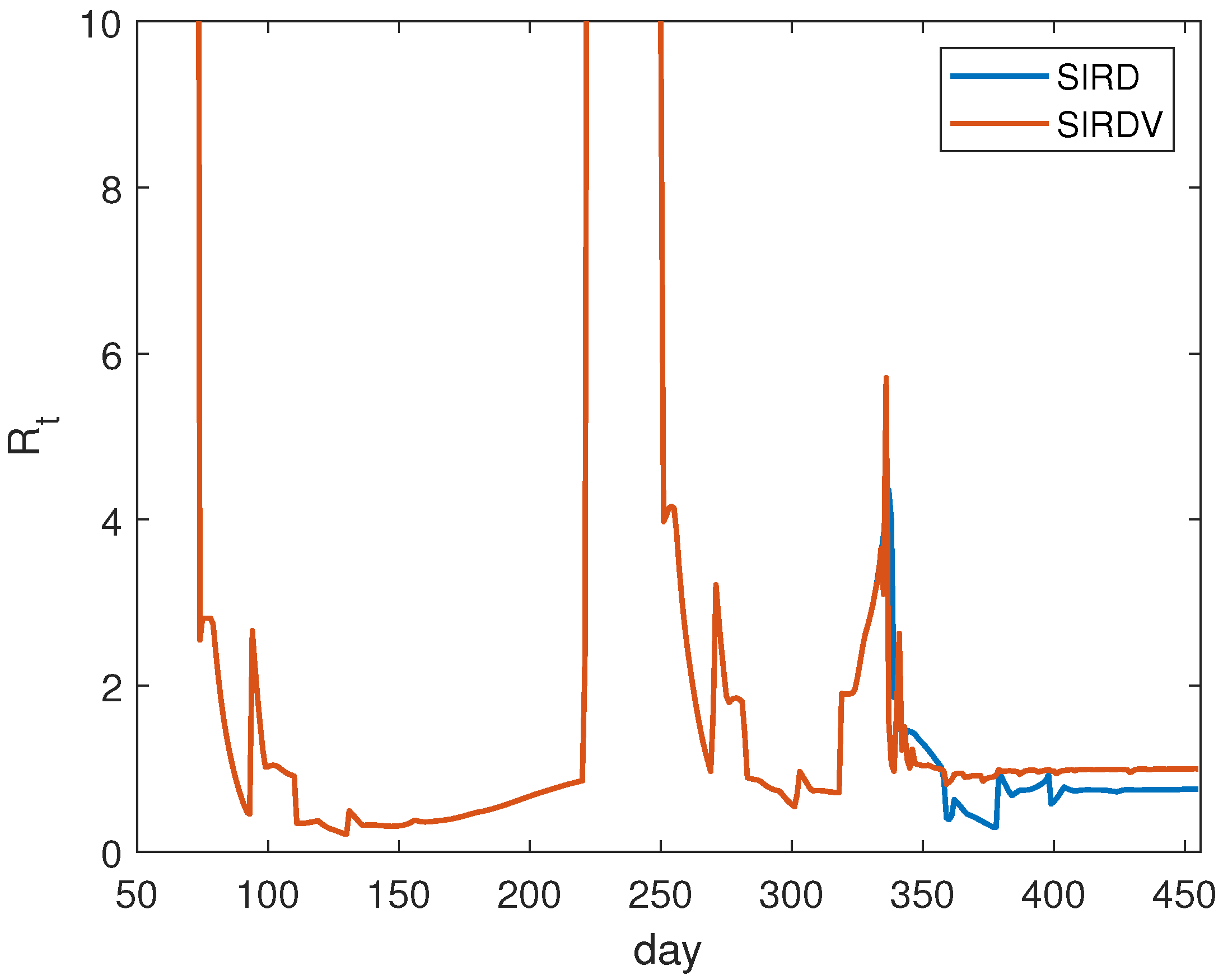
The analysis of $R_t$ is performed with the same technique presented in the previous section for ISR. The numerical results are plotted in Figure 6. Here, the considered time interval starts from 21 March 2020, 50 days following the detection of the first infection. In this case, we notice the presence of high peaks. This is a numerical effect because the peaks correspond to the time periods in which a low number of infections are registered (see Figure 4). In this situation, the numerical estimation of $R_t$ does not result accurately.

4. Pandemic Containment Measures Effects Comparisons

The most influential pandemic containment measure is the vaccination campaign, which affects the contact frequency reduction described by the function $\beta$.

In ISR, the vaccination campaign was very effective because most of the population had received two doses of a vaccine by 30 April 2021. At the same time, the pandemic containment measures during the vaccination period were less restrictive with respect to the lockdown periods; for these reasons, it is possible to notice a substantial difference between the SIRD and the SIRDV model in ISR. In the SIRD model, the combination of the absence of the vaccination campaign with a high $\beta$ value caused an additional infection wave.

In GBR, the vaccination campaign was less effective because most of the population had received only one dose of vaccine, while simultaneously, the pandemic containment measures were more stringent than in ISR during the vaccination campaign. From Figure 5, we can deduce that, without a vaccination campaign, the infected curve does not substantially increase in the short time because social distancing measures were still adopted in GBR in such a period, corresponding to a low value for $\beta$. However, in the medium and long time, we expect a spread increment in both cases with and without vaccination, especially if restrictions are released.

The crucial issue for the model is the function $\beta \left(t\right)$. Its values depend on specific restriction measures. It is possible to recognize four levels of restrictions in each country: total opening, corresponding to an absence of restrictions; partial opening, which implies an opened but controlled phase to isolate the infected individuals; partial closure, describing a not-totally restrictive situation; lockdown, which is the most restrictive level. In

Table 5. GBR (left table) and ISR (right table) function $\beta \left(t\right)$ values related to the restriction measures.

Policy Measure	$\mathit{\beta }$	Value	Policy Measure	$\mathit{\beta }$	Value
Total opening	${\beta }_0$	0.3746 d${}^{-1}$	Total opening	${\beta }_0$	0.7215 d${}^{-1}$
Partial closure	${\beta }_1$	0.0483 d${}^{-1}$	Lockdown	${\beta }_1$	0.0262 d${}^{-1}$
Lockdown	${\beta }_2$	0.0183 d${}^{-1}$	Partial opening	${\beta }_2$	0.1446 d${}^{-1}$
Partial opening	${\beta }_3$	0.3239 d${}^{-1}$	Partial closure	${\beta }_3$	0.0467 d${}^{-1}$
Partial closure	${\beta }_4$	0.0771 d${}^{-1}$	Partial opening	${\beta }_4$	0.0969 d${}^{-1}$
Lockdown	${\beta }_5$	0.0393 d${}^{-1}$	Partial closure	${\beta }_5$	0.0645 d${}^{-1}$
Partial opening	${\beta }_6$	0.1054 d${}^{-1}$	Lockdown	${\beta }_6$	0.0444 d${}^{-1}$
Partial closure	${\beta }_7$	0.0583 d${}^{-1}$	Partial opening	${\beta }_7$	0.1379 d${}^{-1}$
Lockdown	${\beta }_8$	0.0254 d${}^{-1}$	Partial closure	${\beta }_8$	0.0808 d${}^{-1}$
Partial closure	${\beta }_9$	0.0409 d${}^{-1}$	Partial opening	${\beta }_9$	0.1261 d${}^{-1}$

, we report the values of $\beta \left(t\right)$ corresponding to the four restriction levels explained before, for both countries analyzed in this study.

In order to have a confirmation of the dependence between the $\beta$ values and the policy measures, a one-way analysis of variance (ANOVA) is performed. To apply this test, the data are organized into several groups representing a sample extracted from a proper population, and each population represents the results of a specific factor level.

In this case, both for GBR and ISR, the factor is the policy measure and its levels are: total opening, partial opening, partial closure, and lockdown. Instead of a sample extracted from a certain population, the $\beta$ values grouped as in

Table 6. $\beta \left(t\right)$ values grouped by total opening, partial opening, partial closure, and lockdown for the two countries.

Policy Measure	$\mathit{\beta }$ Values for GBR	$\mathit{\beta }$ Values for ISR
Total opening	0.3746 d${}^{-1}$	0.7215 d${}^{-1}$
Partial opening	0.1054 d${}^{-1}$, 0.3239 d${}^{-1}$	0.0969 d${}^{-1}$, 0.1261 d${}^{-1}$, 0.1379 d${}^{-1}$, 0.1446 d${}^{-1}$
Partial closure	0.0409 d${}^{-1}$, 0.0483 d${}^{-1}$, 0.0583 d${}^{-1}$, 0.0771 d${}^{-1}$	0.04675 d${}^{-1}$, 0.0645 d${}^{-1}$, 0.0808 d${}^{-1}$
Lockdown	0.0183 d${}^{-1}$, 0.0254 d${}^{-1}$, 0.0393 d${}^{-1}$	0.0262 d${}^{-1}$, 0.0444 d${}^{-1}$

have been used.

The Fisher statistic (F) value is computed both for GBR and ISR, and it is compared with the quantile of order 0.95 of the Fisher distribution with (3,6) degrees of freedom ($f_{0.95}^F(3,6)=4.7571$). The results are reported in

Table 7. ANOVA test results for GBR and ISR.

ANOVA Test Results
	GBR	ISR
p-value	0.0095	3.61 $\times {10}^{-7}$
F	9.97	362.36

.

It is evident that there is a strong dependence of the $\beta$ values on the policy measures, because of a very low significance level (p-value).

Since the number of $\beta$ values, grouped according to the policy measures, is not so high, we performed the ANOVA test also in a non-parametric way, by means of the Kruskal–Wallis test. The results are reported in

Table 8. Kruskal–Wallis test results for GBR and ISR.

Kruskal–Wallis Test Results
	GBR	ISR
p-value	0.0424	0.0424
Statistics	8.18	8.18

.

In this case, the dependence of $\beta$ on the policy measures is still strong, but with a higher p-value. We remark that the same values both for GBR and ISR are obtained because the Kruskal–Wallis test works with ranks instead of data, and in this case, the statistic results are similar.

Thanks to these considerations, the values in Table 6 can be useful initial guesses for predicting the pandemic trend based on the particular policy measures applied by the governments.

5. Conclusions

In this paper, a data analysis of the evolution of the pandemic in two different countries, GBR and ISR, devising a suitable epidemic mathematical model, was carried out. In [7], a more basic time-delayed deterministic model was introduced, but no applications were provided. Here, we have extended such a model by considering a non-constant contact frequency and by contemplating also the presence of vaccinated people. Moreover, the model has been applied to GBR and ISR considering both vaccinated and not-vaccinated individuals and taking into account the several waves of infection over a long time period. A crucial point is the presence of time delays, giving the possibility of modeling the temporal dynamic of incubation, healing, and death, and to describe the real event sequences during the illness’ evolution. The presence of a non-constant contact frequency allows for the modeling of several waves of infection due to different containment policies. Moreover, the parameters have been calibrated on real data by a fitting procedure.

Finally, a set of parameters has been obtained to predict the pandemic trend based on the policy measures adopted by the government. A confirmation of the dependence between the values of $\beta$ and the policy measures was completed by the ANOVA and the Kruskal–Wallis tests. The obtained results could be a way to help governments endorse valid strategies in the context of disease surveillance; indeed, the results seem very promising from a predictive point of view, and can be adopted to make confident predictions in medium times.