Tracking a Well Diversified Portfolio with Maximum Entropy in the Mean

Abstract

In this work we address the following problem: Having chosen a well diversified portfolio, we show how to improve on its return, maintaining the diversification. In order to achieve this boost on return we construct a neighborhood of the well diversified portfolio and find a portfolio that maximizes the return in that neighborhood. For that we use the method of maximum entropy in the mean to find a portfolio that yields any possible return up to the maximum return within the neighborhood. The implicit bonus of the method is that if the benchmark portfolio has acceptable risk and diversification, the portfolio of maximum return in that neighborhood will also have acceptable risk and diversification.

1. Introduction and Preliminaries

Consider a collection of n assets and let us denote by $\{{\rho }_k:k=1,\dots ,n\}$ the collection of random rates of return of the collection, and by ${\mathit{r}}_a=(r_1,\dots ,r_n)$ the vector of expected return of these assets, that is $E\left[{\rho }_k\right]=r_k,k=1,\dots ,n$. A portfolio with no short positions consists of a vector $\mathit{w}=(w_1,\dots ,w_n)$ such that $⟨\mathit{w},\mathit{u}⟩=1$ and the expected return of the portfolio is given by $⟨\mathit{w},{\mathit{r}}_a⟩$. Here $\mathit{u}=(1,\dots ,1)$. The class $\mathcal{P}$ of admissible portfolios is defined by $\mathcal{P}=\{\mathit{w}\in {\mathbb{R}}^n:0\le w_k\le 1,⟨\mathit{w},\mathit{u}⟩=1\}.$

An investor interested in obtaining the maximum possible return on her investment needs to solve the following problem:

$$\mathrm{F}\mathrm{i}\mathrm{n}\mathrm{d}\mathit{w}\in {\mathbb{R}}^n\mathrm{a}\mathrm{t} \mathrm{w}\mathrm{h}\mathrm{i}\mathrm{c}\mathrm{h}max\{⟨\mathit{w},{\mathit{r}}_a⟩:\mathit{w}\in \mathcal{P}\}\mathrm{i}\mathrm{s} \mathrm{r}\mathrm{e}\mathrm{a}\mathrm{c}\mathrm{h}\mathrm{e}\mathrm{d}.$$

Certainly, this problem has a solution and it is a corner of $\mathcal{P}$. However, this solution is not satisfactory because it ignores some essential issues. Most notably, neither the risk nor the diversification of the portfolio is taken into consideration. There are many ways of setting up a satisfactory (risk, return) balance, and each one of them leads to a solution to the problem. The classical, and most widely used, mean-variance solution by [1] has been known for long to be highly sensitive to parameter estimation errors (e.g., of covariance matrix and especially mean vector of assets returns, see [2]). Several solutions have been proposed for a robust portfolio optimization within this paradigm based on a trade-off of risk and return [3].

The other relevant issue related to the classical Markowitz proposal is the diversification issue. Diversification appears to be an intuitive concept but as with the notion of risk, there does not seem to exist an agreement on how to specify and measure it. From a practitioner perspective, it is widely accepted that a well-diversified portfolio is one where shocks to individual components do not heavily affect the overall performance of the portfolio. This qualitative definition translates in the mean-variance model to an increase in the number of uncorrelated constituents in the portfolio, as it is clear that the larger the number of (uncorrelated) assets the lower the overall variance of the portfolio, and this can be driven to almost zero in an equally weighted portfolio. However authors such as [4] show that in the case of equity mutual funds in spite of the huge number of stocks they hold (more than 100 in many cases) their portfolios are not perfectly diversified, in terms of risk reduction; reference [5] show that in non-Gaussian return distributions, increasing portfolio sizes could not reduce monotonically large risks, and instead a lower number of assets could improve diversification in a bear market. In any case, for the practitioner diversification of a portfolio is still tied to a play with size (number of assets) and approximate weights to uniform distribution. A recent extensive review of the research literature dealing with the relation of number of assets and portfolio diversification is given in [6], and a more general review of diversification in portfolio theory, with focus on its defining principles, usefulness and measurement is given in [7].

Supervised methods to achieve diversification based on risk reduction, such as the MV optimization approach for minimizing the variance, in practice tend to concentrate on very small subsets of the portfolios of interest (more often than not, on a single asset), and this goes against the former accepted notion of diversification, which asks for a reasonable number of assets with similar weights in the portfolio. A prior proposal in which diversification is taken into account along with risk and return tradeoff is that of [8]. They minimize an entropy divergence between the unknown portfolio and that of the naive portfolio subject to return-risk constraint. In this way they achieve a shrinkage towards the maximum diversification as high as possible while maintaining the risk-return constraint. The use of entropy as a measure of diversification in portfolio selection has been validated previously in [9].

Our proposal goes in a related, but quite different direction. We start from a portfolio that satisfies some benchmarking criterion in terms of diversification and risk tolerance, define an acceptable region in portfolio space about the benchmark, and then solve a constrained return maximization problem within that acceptance class of well diversified portfolios. This constrained linear programming problem is an alternative way to achieve shrinkage towards the benchmark.

To be explicit, let us denote by $\mathit{w}\left(d\right)=(w_1\left(d\right),\dots ,w_n\left(d\right))$ the well diversified benchmark and define the set of admissible portfolios by

$$\mathcal{A}=\{\mathit{w}\in \mathcal{P}:a_k=w_k\left(d\right)-l_k\le w_k\le w_k\left(d\right)+u_k=b_k,k=1,\dots ,n\}.$$

(1)

It is the specification of the $l_k$, $u_k$ that determines the risk for the portfolios in $\mathcal{A}$. Consequently the focus of our attention is on the following problem

Problem 1.

Determine a portfolio ${\mathit{w}}^{*}\in \mathcal{A}$ at which $⟨{\mathit{w}}^{*},{\mathit{r}}_a⟩$ reaches its maximum possible value. That is, find

$${\mathit{w}}^{*}=argmax\{⟨\mathit{w},{\mathit{r}}_a⟩:\mathit{w}\in \mathcal{A}\}.$$

For the solution of this problem we will use the method of maximum entropy in the mean (MEM). For this consider [10]. MEM uses the standard entropy maximization method as a stepping stone to solve ill-posed, constrained, linear inverse problems. It is here where our approach differs from that of [8]. They use a cross-entropy minimization procedure under mean variance constraints to obtain a portfolio with good diversification properties. We use the MEM to solve a sequence of constrained linear equations as a way to solve a constrained linear programming problem by a variant of the interior point approach. The mathematics of this approach was initially worked out in [11]. As mentioned above, for us the constraints come from a preassigned band about the benchmark well diversified portfolio, and at the end we shall end with the portfolio that has a maximal return in the region of well diversified portfolios. We remark that we do not strive for efficiency in the Markowitz (risk, return) sense. Instead we start from a well diversified portfolio and improve its return while maintaining a high degree of diversification. Thus, our portfolios are efficient in the sense that it provides the highest possible returns at a given level of diversification.

The process is as follows: Starting with $r\left(d\right)=⟨\mathit{w}\left(d\right),{\mathit{r}}_a⟩$ we increase the return in small steps and solve

Problem 2.

Find $\mathit{w}\left(r\right)$ such that

$$\begin{array}{c}\hfill ⟨\mathit{w}\left(r\right),{\mathit{r}}_a⟩=r\\ \hfill ⟨\mathit{w}\left(r\right),\mathit{u}⟩=1\\ \hfill a_k\le w_k\left(r\right)\le b_k.\end{array}$$

This is the problem to be solved with MEM. We increase r in small steps until no solution to this problem exists. The last r for which the interior point method has a solution is an approximate solution to the linear programming problem. We explain how this is done in Section 2. In Section 4 we report our numerical examples, and for that we first explain in Section 3 how the admissible portfolios are specified. Section 5 concludes.

2. The Maxentropic Solution to Problem 2

Instead of solving an algebraic problem, we consider a linear, inverse ill-posed problem consisting of determining a probability measure P on $\mathcal{A}={\prod }_{k=1}^n[a_k,b_k]$ such that $\mathit{w}\left(r\right)=E_P\left[\mathit{X}\right]$ satisfies Problem 2. Here $\mathit{X}:\mathcal{A}\to \mathcal{A}$ is the identity mapping. On a $\sigma$-algebra of Borel sets on $\mathcal{A}$ we consider the reference measure $Q={\prod }_{k=1}^n\left({ϵ}_{a_k}\left(d{x}_k\right)+{ϵ}_{b_k}\left(d{x}_k\right)\right)$ which puts unit mass at the vertices of $\mathcal{A}.$ The reasons behind this choice are twofold: On the one hand, the computations are simple, and on the other, is the fact that any point in any of the intervals is a convex combination of its extreme points. Before continuing, note that any $P<<Q$ can be written as $Q={\prod }_{k=1}^n\left((1-p_k){ϵ}_{a_k}\left(d{x}_k\right)+p_k{ϵ}_{b_k}\left(d{x}_k\right)\right)$. In particular, the entropy $S_Q\left(P\right)$ of the probability P with respect to the reference measure Q is given by

$$S_Q\left(P\right)=-{\int }_{\mathcal{A}}\left(\frac{dP}{dQ}\right)ln\left(\frac{dP}{dQ}\right)dQ=-\sum _{k=1}^n\left((1-p_k)ln(1-p_k)+p_{k}ln{p}_k\right).$$

(2)

Note now as well that:

$$w_k\left(r\right)=(1-p_k)a_k+p_k{b}_k,k=1,\dots ,n.$$

(3)

It is to find the appropriate $p_k$ that we use the method of maximum entropy. Our problem consists of

Problem 3.

Find $P^{*}$ such that

$$\begin{array}{c}{P}^{*}=argmax\left\{S_Q\left(P\right)\right\}=argmax\left\{-\left(\sum _{k=1}^n(1-p_k)ln(1-p_k)+p_{k}ln{p}_k\right)\right\};\\ subject to the constraints\left\{\begin{array}{c}{E}_P\left[⟨\mathit{X},{\mathit{r}}_a⟩\right]=r\\ E_P\left[⟨\mathit{X},\mathit{u}⟩\right]=1\end{array}\right.\end{array}$$

Note that the last constraint in Problem 2 is automatically taken care of by this problem set up. It is a routine calculation to verify that the solution to Problem 3 is given by

$$p_k^{*}=\frac{e^{-({\lambda }_1^{*}{b}_k+{\lambda }_2^{*}{b}_k{r}_k)}}{e^{-({\lambda }_1^{*}{a}_k+{\lambda }_2^{*}{a}_k{r}_k)}+e^{-({\lambda }_1^{*}{b}_k+{\lambda }_2^{*}{b}_k{r}_k)}}.$$

(4)

The Lagrange multipliers are to be found minimizing the (dual entropy) function

$$({\lambda }_1,{\lambda }_2)\to \Sigma ({\lambda }_1,{\lambda }_2)=\sum _{k=1}^{n}ln\left(e^{-({\lambda }_1{a}_k+{\lambda }_2{a}_k{r}_k)}+e^{-({\lambda }_1{b}_k+{\lambda }_2{b}_k{r}_k)}\right)+{\lambda }_1+{\lambda }_{2}r.$$

(5)

This is a strictly convex function on ${\mathbb{R}}^2$. Once the minimizing values ${\lambda }_1^{*},{\lambda }_2^{*}$ have been determined they are substituted in (4), and then the desired portfolio is given by

$$w_k\left(r\right)=a_k(1-p_k^{*})+b_k{p}_k^{*}.$$

(6)

The existence of the minimizer is equivalent to the existence of $\mathit{w}$ in the interior of $\mathcal{A}$ achieving that return. When the optimization problem has no solution, the minimizer tends to infinity (in the Appendix A we explain why that happens).

To find the portfolio in $\mathcal{A}$ that maximizes the return fix some step size $\delta$ and consider $r_0=r\left(d\right)$ and $r_s=r\left(d\right)+s\delta =r_{s-1}+\delta$. If for some $s_0$ there is a portfolio $\mathit{w}\left(r_{s_0}\right)$ of return $r_{s_0}$ but no portfolio of return $r_{s_0+1}=r_{s_0}+\delta ,$ we stop and the maximum possible return is between $r_{s_0}$ and $r_{s_0}+\delta ,$ that is our estimation error is smaller than $\delta .$ Here the problem solver must choose between increasing r fast and lowering the approximation error.

3. The Well Diversified Portfolio Selection in Practice and Related Issues

As we mentioned above, the two first stages of the problem consist of deciding upon a well diversified benchmark, and then to build the admissible set about it. After that comes the optimization routine described in Section 2.

3.1. Choosing a Well Diversified Portfolio

As argued in the Introduction an accepted benchmark for a diversified portfolio, in practice, is the naive portfolio, which assigns weight $w_k\left(d\right)=1/n$ to each of the n assets. Another choice of reasonable well-diversified portfolio, close in nature to the naive and which somehow reflects the market preferences, is the relative capitalization portfolio, which assigns weight $w_k\left(d\right)=C_k/\left({\sum }_{j=1}^n{C}_j\right)$ to the k-th asset, with $C_k$ being its market capitalization.

3.2. The Admissible Portfolios

Denote by $\mathcal{R}$ our preferred risk measure. Suppose that it is a differentiable function, and let $\mathcal{R}\left(\mathit{w}\right(d\left)\right)$ be the risk of the well diversified portfolio, and $\mathcal{R}\left(\mathit{w}\right)$ the risk of a portfolio in the admissible set $\mathcal{A}$. In the notations of (1) note that:

$$|\mathcal{R}\left(\mathit{w}\right)-\mathcal{R}\left(\mathit{w}\left(d\right)\right)|\le \parallel \nabla \mathcal{R}\left(\mathit{w}\left(d\right)\right)\parallel su{p}_k|u_k-l_k|=\parallel \nabla \mathcal{R}\left(\mathit{w}\left(d\right)\right)\parallel su{p}_k|b_k-u_k|.$$

we are using the standard $\parallel \mathit{V}\parallel$ to denote the Euclidean norm of the vector $\mathit{V}.$ It certainly makes sense to consider $l_k<w_k\left(d\right)$ so that $a_k>0$. So, it suffices to consider $l_k=u_k=\alpha ·w_k\left(d\right)$, for $0<\alpha <1$ and all k, which certainly yields $\parallel \nabla \mathcal{R}\left(\mathit{w}\left(d\right)\right)\parallel su{p}_k|u_k-l_k|<ϵ$, and this incorporates our tolerance to the risk beyond that of the benchmark. In our experiments we will try different values for $\alpha$ to evaluate the impact on varying the width of the band around the well diversified benchmark.

3.3. Dissimilarity Measures between the Initial and the Final Portfolios

As the portfolios that we deal with admit no short positions they can be regarded as probabilities. In the literature there are many ways of measuring distances between two probabilities or to quantify how different they are (see, e.g., [12]). Here we shall mention only two measures. First a true distance between probabilities, the Jeffreys distance [13], and second a standard measure of dissimilarity, namely the Kullback–Leibler divergence [14].

The Jeffreys distance between two discrete probability laws $\mathit{w}\left(1\right)$ and $\mathit{w}\left(2\right)$ is defined as:

$$d_J^2(\mathit{w}\left(1\right),\mathit{w}\left(2\right))=\sum _{k=1}^n{\left(\sqrt{w_k\left(1\right)}-\sqrt{w_k\left(2\right)}\right)}^2.$$

(7)

Of course, there is the standard Kullback–Leibler divergence, which is a measure of dissimilarity between probabilities used in [8] to quantify how different is $\mathit{w}\left(1\right)$ from $\mathit{w}\left(2\right)$. It is given by:

$$K(\mathit{w}\left(1\right),\mathit{w}\left(2\right))=\sum _{k=1}^n{w}_k\left(1\right)ln\left(\frac{w_k\left(1\right)}{w_k\left(2\right)}\right).$$

(8)

It rapidly follows from Jensen’s inequality that despite of the fact that the Kullback–Leibler divergence is not a distance (it is neither symmetric nor does it satisfy the triangle inequality), it nevertheless satisfies

$$K\left(\mathit{w}\right(1),\mathit{w}(2\left)\right)\ge 0,\mathrm{a}\mathrm{n}\mathrm{d}K\left(\mathit{w}\right(1),\mathit{w}(2\left)\right)=0\iff \mathit{w}\left(1\right)=\mathit{w}\left(2\right).$$

We shall use these two to tell how different the maximum return portfolio ${\mathit{w}}^{*}$ is from the well diversified portfolio $\mathit{w}\left(d\right).$

3.4. The Diversification Index

A diversification index provides us with an intrinsic measure that tells us how well diversified a given portfolio index is. If the naive portfolio is taken as the universal benchmark, the Kullback–Leibler divergence defined in (8) can also be considered a diversification index. This is the approach used by [8]. However, there are other indices. For the numerical examples developed below, we use the Kullback–Leibler divergence and the Herfindahl diversification index. This is an intrinsic measure of diversification commonly used to measure how well diversified a portfolio is. For a portfolio $\mathit{w}$ it is given by:

$$H\left(\mathit{w}\right)=\sum _{k=1}^n{w}_k^2.$$

(9)

Since the Herfindahl index of the naive portfolio made up of n assets is $1/n$, the closer that $H\left(\mathit{w}\right)$ is to $1/n$, the better diversified the portfolio is. The Herfindahl index has enjoyed for quite some time a reputation of superior benchmark for market concentration indices among economists and public-policy analysts; see [15] for a review on this index.

For each of the examples below we shall compute the intrinsic diversification index before and after the return maximization process, as well as the two measures of dissimilarity detailed above.

4. Numerical Examples

This section is divided into three parts. In the first part we apply the two criteria for choosing a well diversified benchmark from Section 3.1 and show explicitly how the method of maximum entropy for benchmark tracking works. That is, we explain how we choose a benchmark and examine the effect of applying the maxentropic procedure to obtain a portfolio of maximum expected return within the admissible class. We perform some simple tests. This could be considered an examination of the performance of an interior point method to solve a linear programming problem.

As the input data for the method depends on market data, that is on the average returns of the collection of assets of the portfolio, in the second section we study the robustness of the procedure by averaging over portfolios held for a rebalancing period of 5 and 20 days. In each case we start from a well diversified portfolio $\mathit{w}\left(d\right)$ with expected return $r\left(d\right)$ at the beginning of the period and end up with a portfolio ${\mathit{w}}^{*}$ of return $r^{*}$ at the end of the rebalancing period. Then we average the initial and final returns for these simulations and perform a variety of performance tests. The reason why some smoothing is expected is the following. If we denote by ${\mathit{r}}^k\left(d\right)$ the vector of initial expected returns of the well diversified portfolio for the k-th simulation and, similarly, denote by ${\mathit{r}}^{*k}={\mathit{r}}^k\left(d\right)+{\Delta }^k$ the vector of maximized returns at the end of the investment period in the k-th simulation, where by ${\Delta }^k$ we denote the improvement in the expected return after the MEM procedure is applied to the well diversified portfolio, then if K denotes the number of simulated rebalancing of portfolios, the expected return of the portfolio which is held constant over the simulations is given by:

$$\sum _{k=1}^K⟨{\mathit{w}}^{*k},{\mathit{r}}^{*k}⟩=\sum _{k=1}^K⟨{\mathit{w}}^k\left(d\right),{\mathit{r}}^k\left(d\right)⟩+\sum _{k=1}^K{\Delta }^k.$$

(10)

This identity explains why, even though for each specific initial return the return of the optimized portfolio improves considerably, when we average over all input/output pairs, the performance looks less impressive than the results of the previous section.

In the third subsection we perform a similar analysis for a non-necessarily well diversified portfolio. The two examples we consider are a Markowitz portfolio [1] and a quintile portfolio [16].

4.1. How the MEM Procedure Works

To illustrate the workings of the maxentropic benchmark tracking, we considered a collection of $n=15$ stocks of companies belonging to the DAX index and obtained their daily close prices for a period of 500 market days from which we computed their expected daily rates of return.

For this collection of assets we consider the following two diversified portfolios: First the naive portfolio, with weights $w_j\left(d\right)=1/15$ and then a portfolio that reflects the market capitalization computed as $C_j=pric{e}_j\times volum{e}_j$ divided by the market capitalization of the collection, that is $w_j=C_i/{\sum }_{i=1}^n{C}_i.$ We refer to this portfolio as the relative capitalization portfolio.

For the numerical examples we considered a uniform band defined by $a_j=w_j\left(d\right)(1-\alpha )$ and $b_j=w_j\left(d\right)(1+\alpha ),$ written in such a way that $\alpha$ could be changed. We considered $\alpha =1/2$ to begin with. The step size $\delta$ is taken initially as 10% of the portfolio (by the rationale that an investor would expect to increase its original investment by that much). However, we incremented the portfolio target return from step to step using the corrected recursion $r_s=r_{s-1}+{\left(0.9\right)}^s\delta$, so that the increments are smaller as the step number s increases.

4.1.1. The Naive Portfolio Is the Benchmark

For each of the 15 stocks, we show in Table 1 its weight in the naive portfolio (the quantity to the left of the |, which is $1/15=0.06667$), and its weight in the portfolio that maximizes return in the admissible band about the naive portfolio (the quantity to the right of the |).

Table 1. Initial weights of the naive portfolio (left) and weights of the portfolio that maximizes return in the admissible band about the naive portfolio (right).

Assets		Weights
1 to 3	0.06667 | 0.07549	0.06667 | 0.08646	0.06667 | 0.07888
4 to 6	0.06667 | 0.06443	0.06667 | 0.08471	0.06667 | 0.08659
7 to 9	0.06667 | 0.07726	0.06667 | 0.04915	0.06667 | 0.05003
10 to 12	0.06667 | 0.08498	0.06667 | 0.04834	0.06667 | 0.05927
13 to 15	0.06667 | 0.05132	0.06667 | 0.04693	0.06667 | 0.05615

The daily rate of return of the naive portfolio is 0.013% which is annualized to 3.3%. After applying the maxentropic procedure the new portfolio has a daily rate of return of 0.024%, which is annualized to 6.15%, that is almost twice as much as that of the naive portfolio.

We mention that the norm of the gradient of the dual entropy was less than ${10}^{-6}$, which means that the constraints are satisfied up to six decimal figures.

The Herfindahl index of the naive portfolio is $H\left(\mathit{w}\right(d\left)\right)=0.06667$ whereas that of maximum return is $H\left({\mathit{w}}^{*}\right)=0.07017$. Both portfolios appear to be quite well diversified. That not much diversification is lost seems intuitive on the basis of basic analysis: $\mathit{w}\to H\left(\mathit{w}\right)$ is a continuous function and the neighborhood about $\mathit{w}\left(d\right)$ is small, so not much diversification appears to be lost.

4.1.2. The Relative Capitalization Portfolio Is the Benchmark

We already explained how to produce a well diversified portfolio for this example. This benchmark is a substitute of the market portfolio in terms of risk-return performance and we assume that it incorporates some market driven notion of diversification. In Table 2 we show the weights of the initial relative capitalization portfolio (left of |) and the weights of the portfolio that maximizes return in the admissible band about the relative capitalization portfolio (right of |).

Table 2. Weights of the well diversified portfolio according to the relative capitalization (left) and weights of the portfolio that maximizes return in the admissible band about the relative capitalization portfolio (right).

Assets		Weights
1 to 3	0.06198 | 0.08190	0.09952 | 0.11952	0.07958 | 0.09957
4 to 6	0.10309 | 0.10137	0.06288 | 0.08288	0.03896 | 0.05896
7 to 9	0.10441 | 0.12439	0.11943 | 0.09943	0.06876 | 0.04876
10 to 12	0.02313 | 0.04313	0.04314 | 0.02313	0.02500 | 0.00663
13 to 15	0.02835 | 0.00835	0.02424 | 0.00424	0.11755 | 0.09775

The average daily rate of return of the initial relative capitalization portfolio is 0.014% which annualizes to 3.7%, which is a bit higher than that of the naive portfolio. The expected daily rate of return of the portfolio that maximizes return in the admissible band is 0.027% which annualizes into 6.9%, again almost twice as much, and the portfolio stays in the preassigned band about the well diversified portfolio. The Herfindahl index of the relative capitalization portfolio is $H\left(\mathit{w}\right(d\left)\right)=0.0842989$ whereas that of maximum return is $H\left({\mathit{w}}^{*}\right)=0.09134554$, a close value to the former hence keeping a similar level of diversification.

4.1.3. The Maximum Return Portfolios in Relation to the Benchmarks

Above we saw that given that the region of the well diversified portfolio in which we maximize returns is small so as not to lose diversification, we need some way to quantify how different the portfolios are. For this we use the dissimilarity measures defined previously. The Jeffrey’s distance between two portfolios $\mathit{w}\left(1\right)$ and $\mathit{w}\left(2\right)$ is computed as indicated in (7) and the Kullback–Leibler divergence is computed as indicated in (8).

• Case I: The benchmark is the uniform portfolio.
  • In this case we have
  • (a) The Jefferys distance is $d_J^2({\mathit{w}}^{*},\mathit{w}\left(d\right))=0.01336581.$
  • (b) The Kullback–Leibler divergence is $K({\mathit{w}}^{*},\mathit{w}\left(d\right))=0.02650156.$

• Case II: The relative capitalized benchmark.
  • In this case we have
  • (a) The Jefferys distance is $d_J^2({\mathit{w}}^{*},\mathit{w}\left(d\right))=0.03748571.$
  • (b) The Kullback–Leibler divergence is $K({\mathit{w}}^{*},\mathit{w}\left(d\right))=0.06747427.$

As one can observe in the two cases the small values in both metrics indicate the closeness of both portfolios.

4.2. The Average Performance of the Procedure in Real Life

In order to illustrate the practical usefulness of the MEM diversified portfolio selection method we performed a large number of randomized backtests on a list of portfolios over multiple historical market datasets obtained on a rolling-window basis. The raw historical market data on a daily period is obtained for two international equity indices: The German DAX from 2009-01-01 to 2019-12-31 (for small size portfolios), and the US SP500 from 2008-12-01 to 2018-12-01 (for big size portfolios). Each historical market data is resample into multiple datasets; each resample is obtained by randomly choosing a subset of the stock names (15 for the DAX index, 50 for the SP500) and randomly choosing a time period of 2 years (or 504 days) over the available long period. We apply a rolling window of length 1 year (252 days) for a walk-forward backtesting where the in-sample and out-of-sample windows are constantly shifted. In the in-sample window we estimate parameter values of each portfolio strategy (e.g., covariance, mean, and others). Using the estimated parameters, the optimal portfolio for each considered model is calculated, and tests its performance in the out-sample window by holding the portfolio with the optimal weights through a specific period. We tested for out-sample holding periods of 5 days (a week) and 20 days (one month). Walk-forward backtesting provides a historical simulation of how each portfolio strategy would have performed in the past. This has a clear historical interpretation and its performance can be reconciled with paper trading (for further details see [17]).

Note that our goal is to determine how the MEM diversified portfolio selection impacts on the performance of the associated diversified benchmark portfolio. Thus, if X is some portfolio selection strategy we denote by MEM_X the MEM diversified portfolio selection on top of X. For our experiments we will consider X to be: naive (i.e., equally weighted portfolio) and capital (the market capitalization based portfolio, each weight computed as $C_j=pric{e}_j\times volum{e}_j$ divided by the market capitalization of the collection, that is $w_j=C_i/{\sum }_{i=1}^n{C}_i$). The respective MEM diversified portfolios will be denoted MEM_Naive and MEM_Cap.

To evaluate the performance of each model, we use the following measures: Sharpe ratio (the ratio between the (geometric) annualized return and the annualized standard deviation), Maximum Drawdown (the maximum loss from a peak to a trough of a portfolio), annual return, annual volatility (as annualized standard deviation of returns), and Sterling ratio (the annualized return over maximum drawdown). We also compute the Herfindahl concentration index for each portfolio as an indicator of diversification relative to the naive portfolio (i.e., a well-diversified portfolio of n assets should have its H-index close to $1/n$). All portfolio backtesting experiments were performed with the R package portfolioBacktest [18].

Results for the German market, where we build portfolios of 15 stocks randomly selected from the DAX and for up to 30 price scenarios are shown in Table 3 (for portfolio rebalancing every 5 days) and Table 4 (for portfolio rebalancing every 20 days). Results for the US market, where we build portfolios of 50 stocks randomly selected from the SP500, and for up to 30 price scenarios, are shown in Table 5 (for portfolio rebalancing every 5 days) and Table 6 (for portfolio rebalancing every 20 days). The bandwidth factor $\alpha$ is fixed at 0.6 (after trying several values ranging from 0.5 to 0.9 and found little variation in the results). Bear in mind that all performance results are average values over all the considered trading scenarios.

Table 3. Performance of portfolios samples of 15 stocks (DAX), rebalance every 5, $\alpha =0.6$.

	MEM_Cap	Capital	MEM_Naive	Naive
Sharpe ratio	0.8198	0.6603	0.9894	0.9829
max drawdown	0.1451	0.1479	0.1323	0.1266
annual return	0.1305	0.1065	0.1617	0.1517
annual volatility	0.1943	0.1947	0.1773	0.1725
Sterling ratio	1.0542	0.8460	1.4459	1.3951
Herfindahl	0.0981	0.0946	0.0724	0.0667

Table 4. Performance of portfolios samples of 15 stocks (DAX), rebalance every 20, $\alpha =0.6$.

	MEM_Cap	Capital	MEM_Naive	Naive
Sharpe ratio	0.8194	0.6634	0.9892	0.9769
max drawdown	0.1453	0.1475	0.1320	0.1263
annual return	0.1312	0.1069	0.1662	0.1512
annual volatility	0.1938	0.1948	0.1779	0.1724
Sterling ratio	1.0511	0.8470	1.4421	1.3905
Herfindahl	0.0981	0.0945	0.0725	0.0667

Table 5. Performance of portfolios samples of 50 stocks (SP500), rebalance every 5, $\alpha =0.6$.

	MEM_Cap	Capital	MEM_Naive	Naive
Sharpe ratio	1.1198	1.1345	1.3937	1.4973
max drawdown	0.1088	0.1055	0.0969	0.0873
annual return	0.1639	0.1599	0.1851	0.1885
annual volatility	0.1578	0.1450	0.1339	0.1302
Sterling ratio	1.8061	1.7519	2.2411	2.3159
Herfindahl	0.0516	0.0482	0.0228	0.0200

Table 6. Performance of portfolios samples of 50 stocks (SP500), rebalance every 20, $\alpha =0.6$.

	MEM_Cap	Capital	MEM_Naive	Naive
Sharpe ratio	1.1099	1.1298	1.3734	1.4913
max drawdown	0.1092	0.1065	0.0969	0.0871
annual return	0.1625	0.1593	0.1871	0.1865
annual volatility	0.1583	0.1452	0.1338	0.1300
Sterling ratio	1.7779	1.7514	2.2283	2.3021
Herfindahl	0.0517	0.0482	0.0229	0.0200

We saw in the first section that the expected return relative to that of the benchmark can be increased by appropriately modifying the portfolio. As we saw in the simulations, realized returns might be smaller than expected returns. Our scenario simulation nevertheless shows that the annual returns of the modified portfolio are larger than those of the benchmark without affecting the diversification. We mention that the other performance measures (Sharpe ratio, maximum drawdown and the Sterling ratio described a few lines above) listed in the tables are satisfactory. It appears that the procedure also decreases the volatility of the maximum return portfolio even though this was not an objective of the maxentropic benchmark tracking procedure.

4.3. The MEM Procedure Applied to a Non Well Diversified Portfolio

As it should be clear, the MEM procedure could be applied to any portfolio, regardless of its being well diversified or not. For this we considered a Markowitz type portfolio and a quintile portfolio. Recall that the quintile portfolio consists of sorting assets from high to low by expected return and selecting the top 20% for long-only positions. The mathematical soundness of this strategy as a solution to robust portfolio optimization is analyzed in [16].

We defined a band about the two chosen portfolios for the purpose of maxentropic approach to return augmentation within the acceptable band about the benchmark. Keep in mind that now the acceptable portfolios near the benchmark are not required to be well diversified. To examine the performance of the method we performed the same tests as those that we applied to the well diversified portfolio. 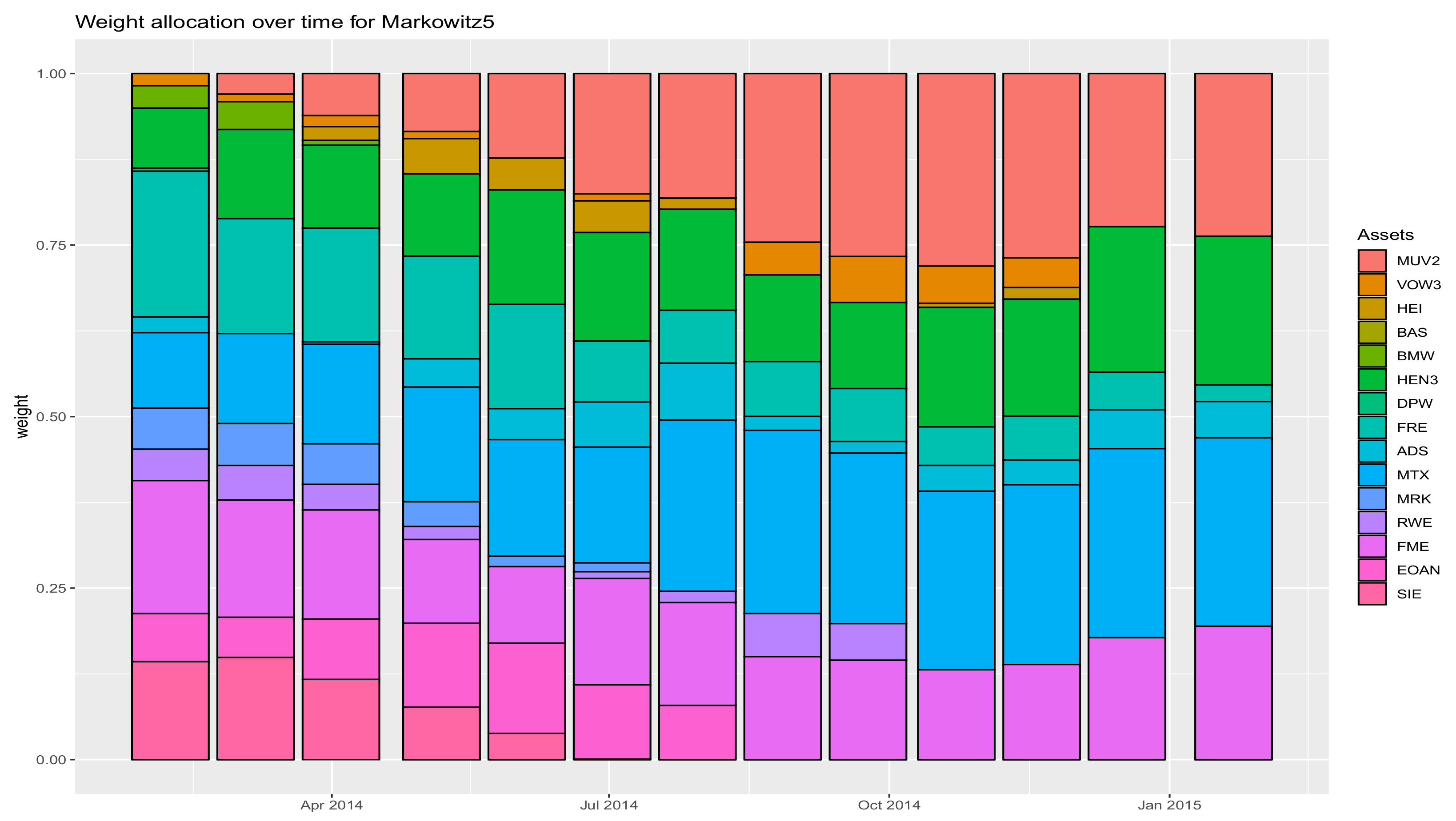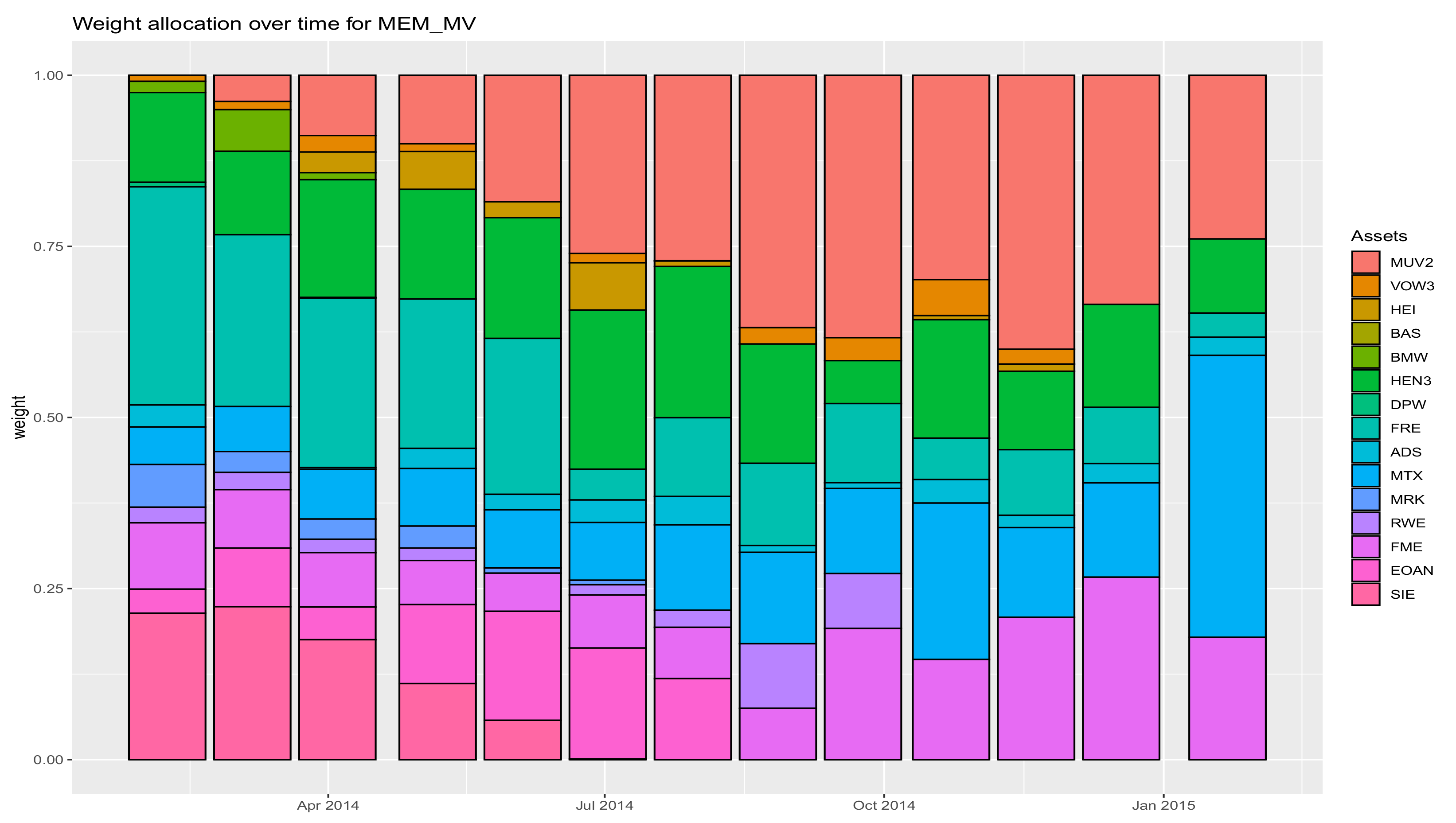The results are shown in the Appendix B, in Table A1 and Table A2 for DAX market and Table A3 and Table A4 for the US market. The nomenclature for the portfolios in these tables is Markowitz5, for the MV or mean-variance portfolio with target return 0.05 (in other words, the minimum variance portfolio to achieve return of 0.05), and quintile, and the respective portfolios after applying MEM for return maximization are termed are MEM_MV and MEM_Quin.

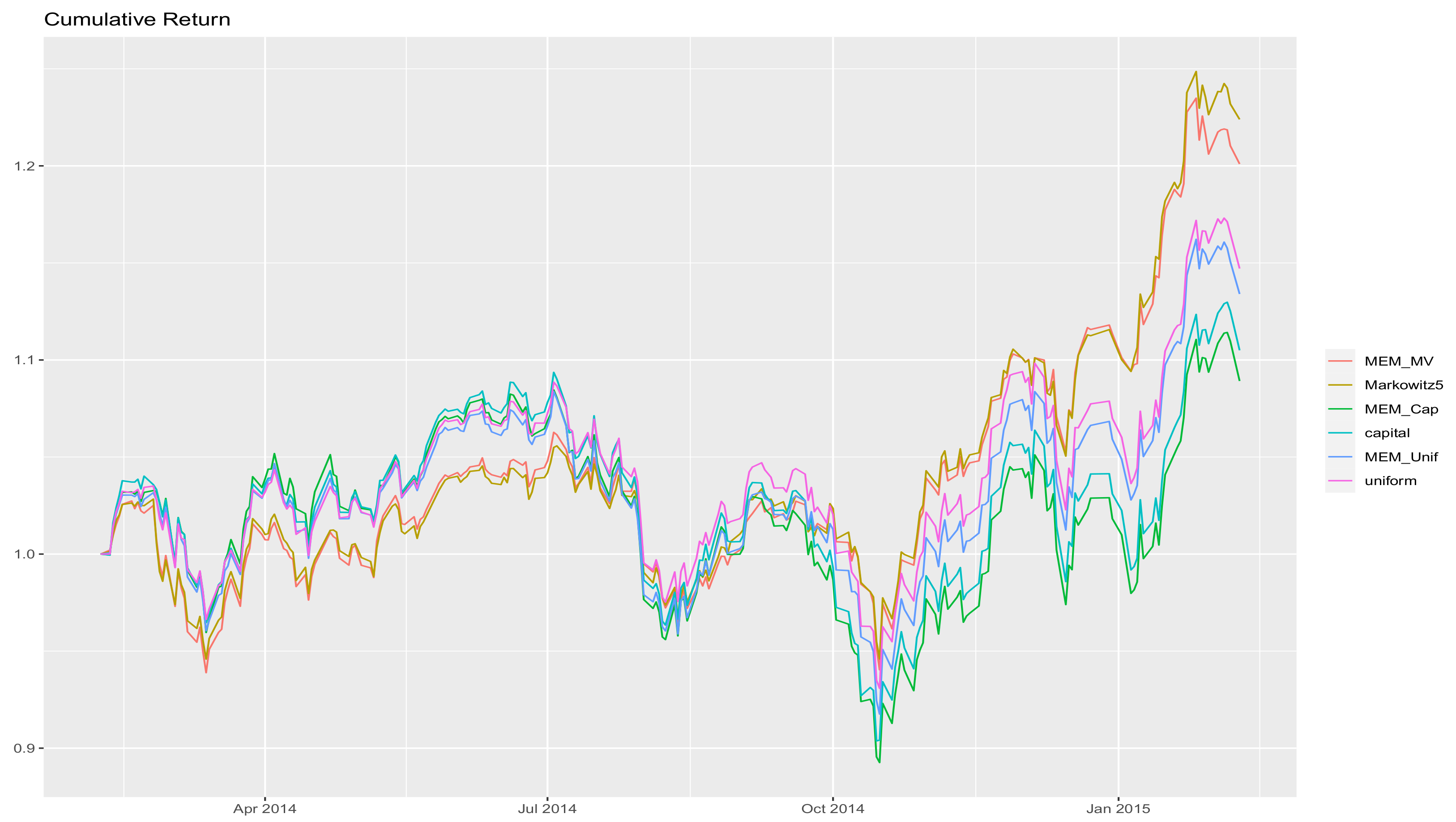
What is somewhat surprising from these tables, is that all performance measures improve after the maxentropic procedure is applied except the Herfindahl diversification index that becomes worse. The lesson seems to be that the maxentropic procedure for benchmark tracking does improve a portfolio optimization strategy keeping in line with the diversification or lack thereof. As an illustration of these facts we include in Appendix B a plot of the cumulative returns of the portfolios obtained in one of the 30 simulations considered for the DAX (Figure A1), as well as pictures of the asset allocation by the MV method (Figure A2) and the asset allocation of the same portfolio optimized by the maxentropic procedure (Figure A3).

5. Concluding Remarks

The first and more obvious comment is that the maxentropic procedure to obtain a portfolio that maximizes the expected return within a band about the benchmark works quite well, regardless of whether the benchmark is well diversified or not. If the benchmark is well diversified, the new portfolio is well diversified as well. This is a reflection of the fact that the diversification index is a continuous function of the portfolio. Moreover, if the market is considered efficient and the relative capitalization reflects the efficiency of the market, then choosing the relative capitalization as a measure of diversification for our benchmark (which is good according to the Herfindahl index), then we maintain the market efficiency and improve upon the return of a well diversified and efficient portfolio.

The general outcome result from our maxentropic optimization is that not only is the expected return increased, also the realized return increases and some standard performance measures, like the Sharpe ratio, the max drawdown and the Sterling ratio, improve as well. This seems to happen not only when the benchmark is well diversified, but at least for the Markowitz and the quintile portfolios, the performance measures report a satisfactory outcome, except concerning the diversification that seems to deteriorate.

To conclude, the procedure seems to open the door to a well behaved benchmark tracking methodology.