Abstract
This study investigates a complex system that describes a non-trivial epidemiological model with integrated internal conflict (interregional migration) on the example of cyclic migration using the software. JetBrains PyCharm Community Edition 2020.3.3, a free and open-source integrated development environment (IDE) in the Python programming language, was chosen as the software development tool. The Matplotlib 3.5 library was used to display the modelling results graphically. The integration of internal conflict into the model revealed significant and notable changes in its behavior. This study’s results prove that not only the characteristics of the interaction factors but also the size of the values determine the direction of migration concerning relation to competitors.
1. Introduction
Despite the global distribution of vaccines, the COVID-19 pandemic still poses a serious threat. The widely available statistics indicate that millions of people have been infected and a large number have died [1,2,3]. This pandemic caused many countries to experience a very negative impact on their economies. Accordingly, many scientists have been involved in predicting the number of possible infected people and assessing the effectiveness of quarantine [4,5,6,7]. To better handle future epidemics, possible scenarios must be planned in advance and responded to accordingly. Due to the growing need to control the COVID-19 pandemic, the number of researchers publishing mathematical modelling work increased [8,9,10].
Mathematical modeling allows researchers to predict the spread of infection and the likely consequences of the epidemic. However, the importance of information regarding health and human life is high [11,12]. The infectious diseases models use basic assumptions or statistics paired with mathematical approaches to calculate disease rate, mortality, and other parameters that describe an epidemic’s nature, provide the information for strategy development and test a model’s effectiveness [13]. The effectiveness of such predictions, accuracy and recency of the data depends on the consideration of all important factors and rules. The more such details are embedded in the model, the more useful it is [14]. Epidemics in different countries have been estimated using the both the classical and generalized susceptible-infected-removed (SIR) model [15,16,17,18,19,20]. Among the works that study SIR-type models, including those that have been published in recent years, it is difficult to find investigations that take into account the regional division of territory and the possibility of migration. Scholars have often generalized and complicated the SIR model itself by introducing additional parameters, even though the model is applied to only one region at a time. One study that does take migration into account was completed by Peter J. Witbooi [21], who used the SEIR model with infected immigrants and recovered emigrants. Further, Min Chen et al. [22] presented the investigations in which population migration to SEIAR for COVID-19 epidemic modeling was included with an efficient intervention strategy. This study, however, also focused on the introduction of additional parameters in the dynamic system that model the arrival or departure of migrants and study the dynamics in one region. Our model allows us to conduct a global analysis of its dynamics in several regions through the introduction of internal conflict interaction. This is a completely different approach, which combines two models instead of improving only one. The proposed model allows the swapping of information and state superposition. Therefore, the following innovations are present in this study. First, it proposes an improved SIR model with some simplifications and modifications to better understand its basic principles and ideas before further inter-regional migration. Second, the influence of internal conflict on the described epidemiological model are investigated. This involves some interregional interaction; migration, similar to the work on the Lotka–Volterra model with cyclic migration, was used [23]. The primary focus of this study is on the rule of redistribution of values, described by the formula of non-linear and non-commutative conflict interaction between two vectors, modified for more rivals.
The presented method has three essential aspects that make it different from previous presented models: (1) our model focuses on the interaction strategy rather than assuming that the strategies are independent [24]; (2) our model takes into account the initial state of the strategy, which is ignored in the existing population dynamics literature [25,26]; (3) in our model, the influence of the environment is considered dynamic in an open system, in contrast to the existing literature, where the capacity of the environment was constant [27].
2. Simulations Based on SIR Model
SIR is one of the simplest polygamous models used to predict the spread of infectious diseases mathematically. This model divides the population into three groups: S—susceptible, I—infectious, R—recovered. The first two groups, susceptible (S) and infected (I), have specific and apparent meanings. Recovered (R), in turn, may have a broader definition. In summary, we can say that R consists of all persons who can no longer fall ill, i.e., those who have recently recovered or died, because none of them will be able to become infected or infect others. The values of each of these groups are time dependent, according to the nature of the disease. The differential equations that describe this model (excluding life dynamics—births and deaths) are as follows:
The SIR model in its original form is not always practical, as it describes the simplest theoretical version of the spread of infection without considering many factors and additional conditions. To solve this problem, the basic model is modified depending on the nature of the epidemiological situation, taking into account various specific factors.
Models of this level of complexity are used to simulate the unfolding of events to assess possible consequences and developing a strategy for counteracting and minimizing casualties [28,29]. In addition, as practice shows, the epidemic scenario is constantly changing, and it is impossible to consider all possible scenarios, so for compliance, models are often modified to obtain new data and try to predict only short periods, ranging from a week to several months. Therefore, the result of the simulation of this model corresponds to the real course of events only during one specific month. A study with similar applications constructed a model that simulated the actual behavior of the spread of COVID-19 in India during April 2020 [30].
3. An Improved SIR Model
As we did not intend to predict the actual epidemiological situation in this work, the SIR model will not be used in its original presentation but with some simplifications and modifications. This will allow us to better understand its basic principles and ideas before further complications in inter-regional migration. The schematic view of the proposed model is presented in Figure 1.
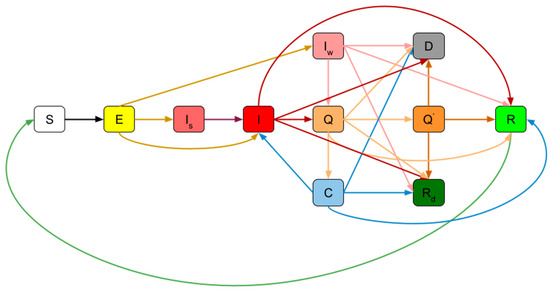
Figure 1.
A schematic view of the proposed SIR model: susceptible (S), non-contagious (E), infected people who ignore the symptoms (I_s), infected (I), asymptomatic infected (Iw), in quarantine (Q), in the intensive care unit (Q’), carriers (C), recovered (R), recovered immobilized (Rd), deaths (D).
The population in the presented SIR model is divided into 11 groups/states, each of which has specific parameters:
- Susceptible (S): includes all those people who are not currently infected but may be in some way in contact with people who have fallen ill.
- Non-contagious (E): includes all persons who have been infected but are asymptomatic and unable to transmit the infection to others.
- Infected people who ignore the symptoms (I_s) include those who have the disease but do not yet seek medical attention. However, as soon as their condition worsens, they still seek help, after which they will be isolated and placed in quarantine conditions.
- Infected (I): includes all infected persons who will soon seek medical help and quarantine. Further, the disease can pass quite quickly, so they can recover while avoiding quarantine, or, alternatively, die from disease complications.
- Asymptomatic infected (I_w): persons infected but have no symptoms, and therefore do not seek medical attention and do not isolate themselves. However, they will be quarantined immediately after returning a positive test result if they have not yet recovered or fallen victim to the epidemic.
- In quarantine (Q): includes all persons quarantined at home or in a medical institution. They are more likely to recover, die, or be transferred to the intensive care unit if their condition worsens.
- In the intensive care unit (Q’): includes persons who have been placed under medical supervision after the deterioration in quarantine. May eventually recover or die.
- Carriers (C): includes all persons who received a negative test result after quarantining but did not, in fact, fully recover. That is, they can infect susceptible individuals without realizing it. Over time, carriers of the infection can fully recover, become ill again, or die.
- Recovered (R): includes individuals who have recovered and can no longer infect anyone. However, with some probability, after a certain period, they may lose their acquired immunity, making them susceptible to infection.
- Recovered immobilized (R_d): includes individuals who have recovered and can no longer infect anyone, but for some reason, they no longer interact with other people. Accordingly, they have no chance of getting sick again.
- Deaths (D): includes all victims of the epidemic.
Differential equations that describe this model, as well as the basic parameters, are as follows:
where is a spreading coefficient of illness and is the rate of loss of immunity in recovered individuals.
is the transition rate from the group (E) to one of the infected conditions.
is a value that determines what proportion of individuals in the transition from group (E) will be infected with symptoms, rather than be asymptomatic; is the proportion of infected people with symptoms that do not ignore them; and is the deterioration rate of people who ignore the disease—the transition to group (I).
is the proportion of infected who will be quarantined; is the proportion of individuals who fall ill multiple times; is the mortality of the infected; is a recovery rate; and is the recovery rate of infected followed by immobilization.
is the mortality of the asymptomatic infected; , are recovery rates; and is the share of detection of infected for further quarantine among people without symptoms.
is the share of quarantined persons who did not fully recover but left isolation (became carriers); is deterioration rate (transition to intensive care); is mortality; and and are recovery rates.
is mortality; and are recovery rates.
is mortality; and are recovery rates.
4. Model of Conflict Interaction of Complex Systems
Conflict, in this study, refers to a physical system consisting of several substances (opponents) , and a particular field Ω in which they exist. We consider conflict one of the most straightforward variants of a complex system, in which this field divides into a finite number of separate regions : . Each substance at a particular point in time is represented by a quantitative characteristic in a particular region, making this system complex. This means that can be described by vectors with non-negative coordinates:
where characterize the substance at the initial moment of time.
The mapping * denotes the iterative law of this conflicting interaction between substances, which is generally unknown. Here we define it according to our intuitive understanding of the physical meaning of substances within the framework of our problem and by the conditions imposed by the studied model.
4.1. The Influence of Internal Conflict on the Described Epidemiological Model
The influence of internal conflict on the described epidemiological model were evaluated in terms of inter-regional interaction and migration, similarly to the Lotka–Volterra model with cyclic migration [20].
For a preliminary description of the principle of migration, which was used as the law of interaction between substances in this study, we used the model of conflict interaction in a system with discrete time between two undestroyed rivals [24]. We were particularly interested in the rule of redistribution of values, described by the formula of non-linear and noncommutative conflict interaction between two vectors, which we later modified to analyze more variables.
where is a normalizing denominator.
Equation (16) describes the change in the quantitative values of substance in regions under the influence of substance with a particular coefficient in the field of interest (the total amount of substance does not change). The result of such interaction depends on the distributions of substances and the coefficient of their interaction. Within the indestructibility of opponents, the interaction is reduced to the movement (outflow) of substances from one region to another. The magnitude of this outflow depends on the value of the intensity rate . Moreover, its sign indicates the direction of movement relative to the magnitude of another substance in the region. These coefficients do not have to be equal for the interaction of with and with , as they describe independent outflows. The first substance can interact with the second more than the second with the first, which makes this rule more universal. With a positive intensity factor during the interaction of substance with (as described by formula (16)), some of the substance in all regions will flow to where there is more substance and vice versa. For example, in the case of two regions, in the region with a larger number of , the amount of will increase, and in the second, where it is less, it will decrease by the same amount. With a larger number of regions, the redistribution is less obvious, but the idea of the principle remains.
It is also worth noting that as a result of such interactions, the total value of each region may change , but not .
In formula (16), normalized (stochastic) vectors are used for calculations. Moreover, since we used natural numbers to describe the amount of substance, before and after the calculations, the required vectors were normalized and normalized, respectively:
where is the number of regions, is absolute amount of substance in region , and is a normalized vector.
When the number of conflicting interaction between rivals was greater than two, the rule of redistribution of values was as follows:
To find the denominator, we used the condition of normalization of the resulting vector:
Next, we described each term by formula (19) and displayed the value of the denominator.
Thus, we obtained the rule of interaction of the opponent with the opponents , and the interaction coefficients :
4.2. Determination of Moving for Population Groups
We then determined which groups of the population are able to move. According to the characteristics of these groups, potential rivals included:
- susceptible (S),
- non-contagious infected (E),
- infected (I),
- infected, ignoring symptoms (),
- asymptomatic infected (),
- carriers (C) and
- recovered (R).
Next, we “placed” the entire population into a specific area and divided it into regions. In addition to satisfying the necessary conditions for integrating conflict into the model, it brings the data closer to real practical conditions. According to the assumptions made in RIS model (Figure 1), each person can belong to one of the eleven groups regardless of region. The conflict itself takes place at every moment of discrete time. Representatives of groups capable of movement interact with each other. However, their migration can also be influenced by immobilization.
Firstly, it was decided to unite some groups together based on like behavior. In our opinion, it would not be entirely correct to consider individuals from each group completely independent and unique in their intentions, given that representatives may have latent signs of infection. Members of such aggregates interact under the influence of typical coefficients or will play the role of a separate substance that can affect the redistribution (migration) of others. Due to the implementation of this principle, this migration model more accurately reflects real migration.
The “do not want to get sick” population group, as the name implies includes all those who consider themselves healthy and are wary of infection, namely the susceptible (S), non-contagious infected (E) and asymptomatic infected () − groups.
The “recovered” population group includes recovered (R), immobilized recovered (), and carriers (C) − . Carriers were included in this category because, according to the model, they are unaware of their ability to spread the infection due to returning a negative test and exhibiting no symptoms, which makes their behavior similar to those with immunity obtained as a result of full recovery. In order to take into account the immobilized’s lack of ability to move, but still allow for the migration of the rest of the recovered, we also highlighted the subset .
Individuals in quarantine (Q) and in the intensive care unit () were classified as (), because the differences between these groups are insignificant.
It was decided not to unite the infected (I) and infected, ignoring the symptoms () groups because the “ideology” of these groups differs significantly—while some are aware of the dangers of the situation, do not waste time and seek help as soon as possible, others do not understand the seriousness of their symptoms and postpone visiting the hospital. This group was a middle ground between not yet contagious infected (E), who in turn consider themselves healthy, and infected with full-fledged symptoms that are difficult to ignore.
The last group, the dead (D), is separate. Following the redistribution rule (20), there can be two types of participants in a conflict interaction. The first, which we call “full participants”, includes those communities and groups that are capable of migration, and their migration influences the migration of others. These include , , (I) and (). The second, ”static participants”, are representatives of those groups that cannot move but can influence the redistribution of others, namely , () and (D).
The above-discussed principles of migration are presented schematically in Figure 2. The direction of each arrow indicates the group or set under the influence of which the participant is migrating from its original side. A bilateral dotted arrow indicates mutual influence on redistribution during conflict interaction of each part. That is, during such a conflict interaction, for example, the “do not want to get sick” group migrates under the influence of the “recovered” and “quarantined” groups, as well as the “infected” and “dead” groups.
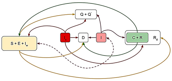
Figure 2.
The basic migration principles indicated for group under the influence of which the participant is migrating by the proposed SIR model: susceptible (S), non-contagious (E), infected people who ignore the symptoms (I_s), infected (I), asymptomatic infected (Iw), in quarantine (Q), in the intensive care unit (Q’), carriers (C), recovered (R), recovered immobilized (Rd), deaths (D).
The state of the whole system automatically adjust, and twelve vectors, one by each group and the vector of the total number of people in the region, as the latter’s value may change as a result of migration. The general algorithm of the program during one bypass in the cycle was as follows:
First of all, we recalculated the vectors within each region according to the formulas in Section 1 in the discrete form:
where is the intermediate moment of evolutionary cycles.
Next, we conducted interaction between the parties to the conflict by pre-forming the vectors of the sets (coordinate addition):
Before performing calculations, all vectors were normalized, and the calculations themselves were performed according to the following formulas:
where . The following conditions were also imposed on the interaction coefficients:
After that, the resulting vectors were de-normed, and the vector of all persons was recalculated by regions
, and the bypass ended.
5. Modelling Results
In this section, we considered the behavior of the created model, simulating different scenarios for the development of events using the program.
The initial distributions were be as follows:
Next, we considered the behavior at different coefficients of conflict interaction and, most importantly, at different signs, because although the magnitude of the interaction is essential, the direction of migration is less so.
5.1. Results of First Example
Firstly, a scenario in which all the coefficients are equal to zero was considered. In this scenario, there is no conflict, but the division into regions remains. The results are presented in Figure 3.
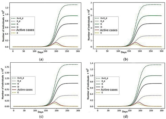
Figure 3.
A scenario in which all the coefficients are equal to zero: (a) Region 1; (b) Region 2; (c) Region 3; (d) Region 4.
In the absence of conflict, we obtained four independent epidemiological models, which were used to investigate the representatives of those groups that cannot move, but were able to influence the redistribution of others (R + R_d), sets of recovered (R), immobilized recovered (R_d), the dead (D), active cases and non-contagious people (E) unable to transmit the infection to others. They were also able to affect overall behavior depending on its size. The final death toll in the regional division decreased by 5920, which, although significant, is only a 0.002% improvement, and so can be ignored.
In the future, we will use mortality to assess the impact of conflict on the model because this metric is simple to understand and informative. From the obtained results, it can be concluded that the behavior of such an epidemiological model, in the absence of external influences, scales proportionally relative to its size.
5.2. Results of Second Example
Another set of parameters were also considered: , and the rest are zero. In such a situation, the group “do not want to get sick” group migrated to regions with more recovered, and both groups of infected ( and ), in turn, tried to distance themselves from them while wanting to be in places with more people in quarantine, although with lower priority (). Recovered, able-bodied people, on the other hand, migrated to regions with fewer deaths and avoid uninfected people, but also with lower priority.
The graph of the general behavior of the model (see Figure 4) shows that the number of active cases increased, though not as smoothly as in the case of no conflict, and then decreased.
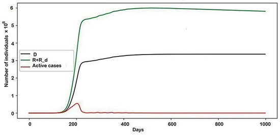
Figure 4.
The behavior of the system in general.
The results of the second example provided much more notable results. Another set of parameters that were unequal to zero was used. The graph of the general behavior of the model (Figure 4) shows that the number of active cases increases, though not as smoothly as in the case of no conflict, and then decreases.
However, as shown in Figure 5, the epidemic did not end there, continuing to rise or fall in the form of damped fluctuations. This, in turn, affected the number of recovered (R + R_d) and dead (D), whose schedules increased for a long time after the peak of the epidemic. As a result of this conflict, the final number of deaths increased by 51,603,004, which is 18% of the death rate in the conventional model.
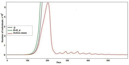
Figure 5.
The pandemic description with parameters set for example two.
The Analysis of Particular Situations in Each Region
The situations in each region were analyzed. First, the regions by the nature of behavior can be divided into two types. The first type includes the first and fourth regions—the situation has stabilized for about 245 and 265 days. Therefore, their total share of the population is about 30%, including only immobile recovered and dead. Their number in these regions was the largest of all regions. Although the initial distribution determined that these two groups made up a total of 51% of the total population, their mobile share of the population was fully distributed among other regions. Prior to the stabilization of behavior in these regions, the worst epidemiological situation was indicated by the highest peak values for each of the groups that form the values of active patients, which explains why these regions recorded the highest number of fatalities, following the migration given by the coefficient , “scared” the recovered able to move. Moreover, they, in turn, being an attractive factor for a set of people who do not want to get sick (), indirectly dragged them despite their desire to avoid illness, in accordance with the coefficient of interaction . This simulation is smaller in modulus than , which caused this behaviour and confirms the importance of its value, especially in scenarios where there are several influencing factors. The modelling results for groups that are able to influence the redistribution of others (R + R_d) and for sets of recovered (R), immobilized recovered (R_d), the dead (D), active cases and noncontagious people (E) unable to transmit the infection to others are presented in Figure 6.
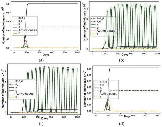
Figure 6.
The graphical results a scenario in which , and the rest are equal to zero: (a) Region 1; (b) Region 2; (c) Region 3; (d) Region 4.
Before the peak of the epidemic, the vast majority of the population belonged to the susceptible (S) group, and therefore were under the influence of conflict interaction for a set of people who do not want to get sick. They tried to move towards the regions with the most significant number of recovered. Since, at this point, the epidemic was just beginning to gain momentum, there are equally few recovered in each region. Due to this, almost the entire population migrated between all regions, which reflects fluctuations in the graphs in Figure 6. Then, after around 200 days, the epidemic peaks, and the most prominent centers are the first and fourth regions. In turn, the second and third regions, despite initially displaying the smallest and largest values, respectively, became almost equal in size after the epidemic. As shown in Figure 6 and Figure 7, they housed the entire mobile part of the population.
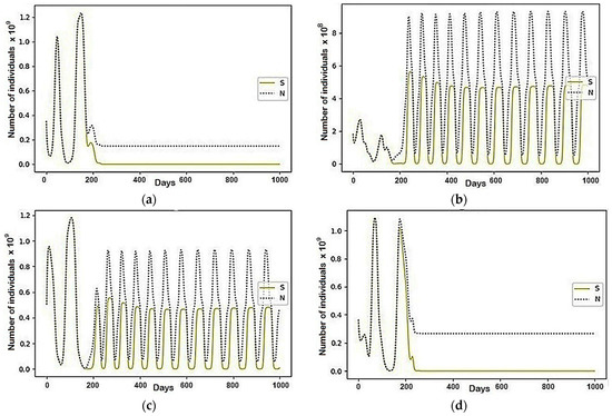
Figure 7.
The modeling results describing the total population size (N) and the population belonging to the susceptible (S) group, where , and the rest are equal to zero: (a) Region 1; (b) Region 2; (c) Region 3; (d) Region 4.
However, questions arise about the causes of such shifts and the coincidence of periods. For now, these questions remain unanswered. In each cycle of such oscillations, all the recovered “ran away” from the susceptible, according to coefficient from the second (third) region to the third (second). They were followed by the susceptible, which provoked the recovered to migrate back, where the number of susceptible decreased. Therefore, modelling processes included those communities and groups that are capable of migration, as well as the groups that their migration can influence, which are a middle ground between not yet contagious infected (E), asymptomatic infected (I_w), infected (I) and infected, ignoring the symptoms (I_s) (see Figure 8). The “static participants” were representatives of those groups that could not move but are able to influence the redistribution of others: the individuals in quarantine (Q) and in the intensive care unit (Q^’) were classified as (Q + Q^’), and set of “recovered” includes (C). The modelling results of how fluctuations affected the groups that made up the total number of active infections are presented in Figure 8 and Figure 9. While large numbers of those infected in the first and fourth regions formed the main wave and peak of the epidemic, residents of the other two regions were responsible for other smaller waves (see fluctuations in Figure 9).
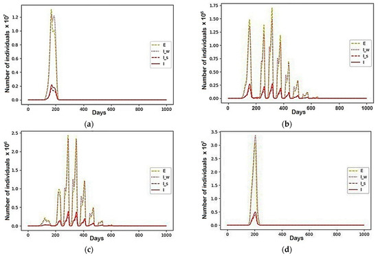
Figure 8.
A scenario in which , and the rest are equal to zero: (a) Region 1; (b) Region 2; (c) Region 3; (d) Region 4.
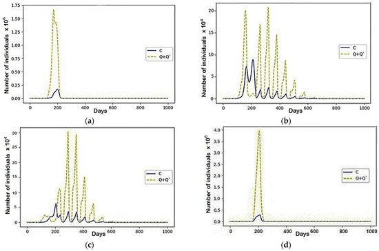
Figure 9.
A scenario in which , and the rest are equal to zero: (a) Region 1; (b) Region 2; (c) Region 3; (d) Region 4.
According to the conflict, migration between regions one and four did not stop, eventually forming fluctuations, which can be explained by the equally low number of deaths after the epidemic, as well as the periods of fluctuations that coincided with the presence of a phase shift (Figure 9).
Analyzing the occurrence of these fluctuations, we can see that after the end of the epidemic in the first and fourth regions, the rate of infection immediately increased. From this, it can be concluded that the sharp end of the epidemic was partly due to the migration of infected to the other two regions. After that, due to the migration of large numbers of people susceptible to infection, there was a further increase in the number of infected in the second and third regions. This increase occurred during several wave oscillations due to the infected migrating between the regions. During the first two fluctuations, their numbers first increased to their greatest values, after which they began to fade.
5.3. Results of the Third Example
A conflict given by the following parameters was considered: , and the rest are equal to zero. Such values present a scenario in which people avoided others who did not want to get sick and regions had large numbers of recovered and dead, but the latter factor was not prioritized. Infected people wanted to be in regions with many people in quarantine and with fewer deaths, not with sick (with the highest priority) or recovered (second place in priority) people. The recovered, in turn, avoid high mortality and gravitate to regions with a predominance of people who do not want to get sick.
In this configuration, as shown in Figure 10, the model behaved in much the same way as in the absence of conflict. This was confirmed by the final number of fatalities, which increased by 2,269,030, which is a deterioration of only 0.8%.
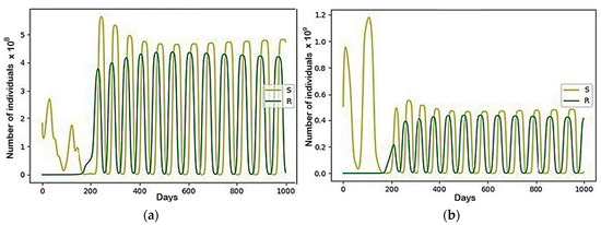
Figure 10.
The modeling results describing the recovered (R) and the susceptible (S) group, where , the rest are equal to zero: (a) Region 1; (b) Region 2.
There are notable differences between this model and the previous models, which can be seen in the graphs of behavior of the susceptible (S) group, the total population size (N), and recovered (R) within individual regions (see Figure A1, Appendix A). Despite the passing of the pandemic peak and the steady decline in morbidity in general, it was at this time that the migratory fluctuations of the recovered and susceptible between all regions began to grow.
This growth can be attributed primarily to a significant increase in the number of recovered after the epidemic peak, which allowed the model to reach a particular value sufficient to intensify the oscillatory process. Further, without sufficient susceptibility in all regions, there were no necessary reasons to migrate between them.
The number of deaths influenced the nature of migration of the recovered during some parts of the growth phase. However, it then ceased to be significant, as we can see that migration continued without preference for a specific region. However, it would not be a surprise to see the isolation of migration in the two regions with the lowest number of deaths. Despite the same values of the coefficients and , this scenario was the first to determine the further behavior of the model. It also revealed that the fluctuations, even after the end of the growth phase, are not homogeneous. It is difficult to say exactly why this occurred. At the end of the epidemic, the only evolutionary change in this model was the constant slight decrease in the number of recovered people able to move, according to the loss of immunity over time. After that, they become susceptible again and are therefore under the influence of opposite migrations.
Again, the reason for such migrations, at the end of the simulation, are the same periods of oscillation and their phase shift. Moreover, as seen in Figure A1 (see Appendix A) and Figure 11, where the group that is able to influence the redistribution of others (R + R_d) and sets of recovered (R), immobilized recovered (R_d), the dead (D), active cases and non-contagious (E) unable to transmit the infection to others are presented, they do not remain constant but meet the conditions necessary for the existence of these fluctuations. We want to note that the approximately uniform distribution of the mobile part of the population after the end of a phase of fluctuation growth between regions, the initial distribution of the sizes of regions occurs.
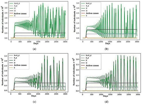
Figure 11.
A scenario in which , and the rest are equal to zero: (a) Region 1; (b) Region 2; (c) Region 3; (d) Region 4.
5.4. Results of the Fourth Example
Examples 2 and 3 clearly show how the impact of internal conflict worsens the epidemiological situation. Migration has led to an increase in deaths. However, in example 3, this growth was not significant, suggesting a positive conflict in a particular configuration.
Parameters were then selected to determine the minimization of infection and, consequently, of the number of victims. The chosen parameter values are presented in Table 1 and the modelling results in Figure 12.

Table 1.
Coefficients of the parameters depending on the case of infection reduction.
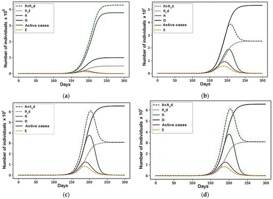
Figure 12.
The case with the parameters represented in Table 1: (a) Region 1; (b) Region 2; (c) Region 3; (d) Region 4.
In this configuration, the “do not want to get sick” population avoided large numbers of infected, dead and quarantined people but gravitated to regions with a large proportion of recovered people, which means a better epidemiological situation. Infected people tried to avoid the “still healthy” so as not to infect them, and they migrated to places where more have recovered or are still in isolation and where fewer have died. The recovered, in turn, avoided high mortality and return to uninfected persons.
The general behavior of this model was identical to that in Figure A2 (see Appendix A). However, in this model, the number of victims decreased by 1,677,739, which is 0.6%, indicating that the situation improved. The modelling results are presented in Figure 12. We want to note that the flow of the recovered after the peak of the epidemic to the first region eventually became the largest. The model behaved very similarly within the third and fourth regions—despite the significant difference in the initial size, at the end of the simulation, their characteristics became almost identical.
During the simulation, other characteristics of the model differ little from the same, but without conflict. No migration fluctuations, as in the previous two examples, occurred. One possible explanation for this is the presence of many factors influencing each side of the conflict (all coefficients are non-zero), which could neutralize migratory fluctuations throughout the system.
5.5. Results of the Fifth Example
In this example, the parameters were selected manually to minimize the epidemic’s effects but without taking into account their detailed interpretation. The chosen parameter values are presented in Table 2 and graphically are presented by Figure 13 and Figure 14 and (see Figure A3 and Figure A4, Appendix A).
Table 2.
Coefficients of the parameters depending on the case of infection effects reduction.
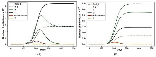
Figure 13.
A scenario with the parameters represented in Table 2: (a) Region 3; (b) Region 4.
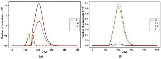
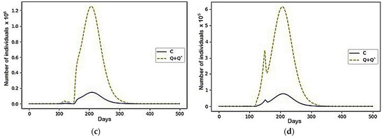
Figure 14.
The case with the parameters represented in Table 2: (a) Region 3; (b) Region 4; (c) Region 3; (d) Region 4.
In this configuration of internal conflict, the number of deaths was reduced by 77,196,596 people, which is a 27% improvement. We want to note that, even before the beginning of the active growth of the number of infected, the resources of the first two regions were almost completely distributed among the third and fourth regions (there were less than 1000 left in each). Then, over several cycles of fluctuations, individuals who avoided infection migrated between them and, with the onset of a more active phase of the epidemic’s growth, fully migrated to the fourth. They behaved similarly and recovered. Thus, at the end of the simulation, the fourth region contained 93.5% of the initial population.
6. Discussion
Recent studies have proposed fractional-order mathematical models focused on describing the dynamic patterns of COVID-19 [31,32,33,34,35,36]. Rezapour et al. analyzed the spread of COVID-19 in Iran using an SEIR model with constant fractional order based on the fractional-order derivative with singular kernel [32]. A five-term dynamical structure was projected to understand the trade-off between the lockdown and the spread of the virus [33]. Other studies also used fractional-order mathematical models to determine a reproduction number of COVID-19 [34] or applied a constant fractional-order model to reveal the transmission dynamics [35]. Rajagopal et al. implemented the SEIRD model to investigate the spread of COVID-19 and compare results with real data [36].
However, the cited works represent only the well-thought-out constant fractional orders, i.e., the same memory indexes used to measure COVID-19 progress. We studied a complex system in the form of time profiles since the model of conflict interaction requires discrete recalculations of quantitative characteristics of parameters in each region. On the one hand, this simplifies the model and eliminates the possibility of obtaining marginal results by classical methods. On the other hand, it expands the possibilities of the model because, as already mentioned, other approaches are forced to limit the study to one region (even if they take into account migration to this region) and do not see the global picture of several regions and their interactions. In addition, our approach was motivated by the fact that migration processes, in contrast to an epidemic, are slower and are not continuous in the classical sense, so discrete recalculations of the number of patients recovered and other factors that vary due to migration, can be adjusted to the model depending on the speed and nature of migration processes.
As part of this work, a complex epidemiological model was built to divide the population into 11 groups (see Figure 1). By examining its behavior by comparing it to several simulations, it was concluded that it is almost independent of the initial distributions that set the starting values of the number of persons. The only variable they affect is the moment of the peak of the epidemic—by varying the initial values, it can be accelerated or delayed. The nature of the behavior model set such parameters as the spread of infection, recovery rates, mortality, and the transition between groups and others with different magnitudes of influence.
Integrating internal conflict into the model has brought about significant and exciting changes in its behavior. First of all, it was found that the signs of the interaction coefficients, which determine the direction of migration relative to rivals and the magnitude of the values, have an important influence. This was especially evident in the framework of the studied principles of migration under the influence of several factors simultaneously. In such cases, a larger module coefficient determines which factor has a more significant impact on establishing the direction of migration. Having studied the model with zero coefficients of conflict interaction, i.e., with only one division into regions, we concluded that its behavior scales proportionally relative to its size in the absence of external influences.
The most interesting results were obtained after conducting simulations with different sets of coefficients. Internal conflict has a significant impact on the behavior of such a system and can both worsen and improve an epidemiological situation.
Migration can take different forms. These include reasonably obvious in the form of smooth relocation from one region to another, the stability of the general situation, and inhomogeneous or homogeneous migratory fluctuations that do not fade. Their principle of appearance remains unknown.
When trying to use the conflict to minimize the consequences of the epidemic, the selection of parameters taking into account the content of their interpretation did not improve significantly. Example 5 showed that migrations with somewhat illogical directions, such as the attraction of the population that is wary of the disease to regions with a higher proportion of infected, lead to a significant reduction in mortality. This reaffirmed that such conflicting interactions in complex systems have a significant impact and do not determine the outcome in advance. The construction of conflicts by interpreting the possible impact of interaction coefficients may not always give the expected result. For now, computer simulation remains the solution.
Regarding the convergence of the model, it should be noted that our main goal was to build a model that considered the impact of migration processes on the spread of the epidemic, and the main impact of such will be regular fluctuations, i.e., epidemic waves we observe. As a consequence of the oscillations (which we see in the graphs), it is impossible to discuss the convergence of the model to any limit values. This is one of the features of our model and differentiates it from other similar models. Note that similar issues have already been discussed in work [28], where it is shown that internal conflict, if considered separately, allows marginal results to be obtained. Dynamic models such as Lotka–Volterra also go to the limit state, but their combination produces models with stable fluctuations that do not allow marginal results to be obtained.
7. Conclusions
The presented model allows a global analysis of the dynamics of the model in several regions to be conducted through the introduction of internal conflict interaction. This is a completely different approach, which combines two models instead of improving only one. Integrating internal conflict into the model brought about significant and notable changes in its behavior. First of all, it was found that the signs of interaction coefficients, which determine the direction of migration relative to rivals, and the magnitude of values have a significant influence.
This was especially evident in the framework of the studied principles of migration under the influence of several factors simultaneously. In such cases, the larger modulus of the coefficient determined which influence factor has the greater weight on establishing the direction of migration. Internal conflict has a significant impact on the behavior of such a system and can both worsen and improve the epidemiological situation.
The migrations themselves, given by population division, can have different forms—from evident and understandable, in the form of smooth relocation from one region to another with the subsequent stability of the general situation, to inhomogeneous or homogeneous migratory fluctuations that do not fade. Their principle of appearance remains unknown.
The main limitations of the model are the difficulties that arise in the selection of system coefficients. In the absence of successful selection, the model does not provide natural dynamics. It is proposed that this problem can be solved by selecting coefficients using neural networks, which will bring the model’s behavior closer to real data, and using the model to predict and provide recommendations for improving the dynamics of morbidity. The authors plan to conduct further research in this direction.
Author Contributions
Conceptualization, I.S., A.N., S.B. and I.M.-K.; methodology, I.S., A.N. and S.B.; software, I.S. and A.N., validation, I.S., A.N., S.B. and I.M.-K.; formal analysis, I.S. and A.N.; writing—original draft preparation, A.N., S.B., I.S. and I.M.-K.; writing—review and editing, I.S., A.N., S.B. and I.M.-K.; supervision, S.B. and I.M.-K. All authors have read and agreed to the published version of the manuscript.
Funding
This research was funded by Ministry of National Defence Republic of Lithuania as a part of the research project Study Support Projects No VI-18, 2 December 2021 (2021–2024), General Jonas Žemaitis, Military Academy of Lithuania, Vilnius, Lithuania. Any opinions, findings and conclusions or recommendations expressed in this material are those of the authors and do not necessarily reflect the view of the funding agency.
Institutional Review Board Statement
The study was conducted according to the guidelines of the Declaration of Helsinki.
Informed Consent Statement
This research there were not used specifical human materials. The research was based on the dataset officially presented as coronavirus (COVID-19) Deaths. Available online: https://ourworldindata.org/covid-deaths (accessed on 8 April 2021).
Data Availability Statement
Not applicable.
Conflicts of Interest
The authors declare no conflict of interest.
Appendix A
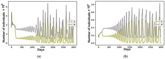
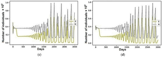
Figure A1.
The modeling results describing the total population size (N) and the population belonged to the susceptible (S) group using the parameters represented in Table 1: (a) Region 1; (b) Region 2; (c) Region 3; (d) Region 4.
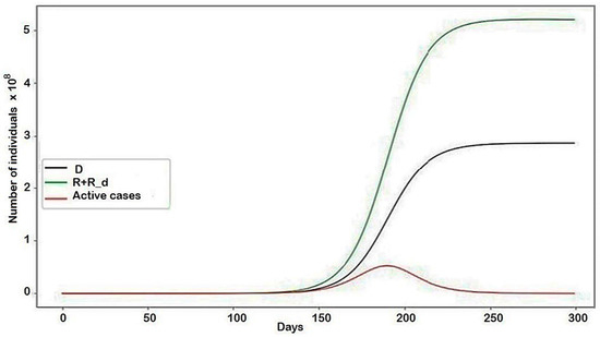
Figure A2.
The modeling results describing the behaviors of the system in general. The conflict is given by the following parameters: , the rest are equal to zero.
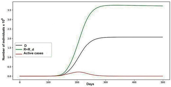
Figure A3.
The modeling results describing the behaviors of the system in general with the parameters represented in Table 1.
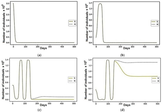
Figure A4.
The modeling results describing the total population size (N) and the population belonging to the susceptible (S) group using the parameters represented in Table 2: (a) Region 1; (b) Region 3; (c) Region 2; (d) Region 4.
References
- Coronavirus (COVID-19) Deaths. Available online: https://ourworldindata.org/covid-deaths (accessed on 8 April 2021).
- Ashish, M.; Nithin, K.R.; Anish, C. Girish Setlur—Modelling and simulation of COVID-19 propagation in a large population with specific reference to India. medRxiv 2020. [Google Scholar] [CrossRef]
- Tušer, I.; Hoskova-Mayerova, S. Emergency Management in Resolving an Emergency Situation. J. Risk Financ. Manag. 2020, 13, 262. [Google Scholar] [CrossRef]
- Božek, F.; Tušer, I. Measures for Ensuring Sustainability during the Current Spreading of Coronaviruses in the Czech Republic. Sustainability 2021, 13, 6764. [Google Scholar] [CrossRef]
- Tušer, I.; Jánský, J.; Petráš, A. Assessment of military preparedness for naturogenic threat: The COVID-19 pandemic in the Czech Republic. Heliyon 2021, 7, e06817. [Google Scholar] [CrossRef]
- Sangodapo, T.O.; Onasanya, B.O.; Mayerova-Hoskova, S. Decision-Making with Fuzzy Soft Matrix Using a Revised Method: A Case of Medical Diagnosis of Diseases. Mathematics 2021, 9, 2327. [Google Scholar] [CrossRef]
- Abro, K.A.; Atangana, A. Numerical and mathematical analysis of induction motor by means of AB–fractal–fractional differentiation actuated by drilling system. Numer. Methods Partial. Differ. Equ. 2020, 11, 22618. [Google Scholar] [CrossRef]
- Atangana, E.; Atangana, A. Facemasks simple but powerful weapons to protect against COVID-19 spread: Can they have sides effects? Results Phys. 2020, 19, 103425. [Google Scholar] [CrossRef]
- Eikenberry, S.E.; Mancuso, M.; Iboi, E.; Phan, T.; Eikenberry, K.; Kuang, Y.; Kostelich, E.; Gumel, A.B. To mask or not to mask: Modeling the potential for face mask use by the general public to curtail the COVID-19 pandemic. Infect. Dis. Model. 2020, 5, 293–308. [Google Scholar] [CrossRef]
- Baud, D.; Qi, X.; Nielsen-Saines, K.; Musso, D.; Pomar, L.; Favre, G. Real estimates of mortality following COVID-19 infection. Lancet Infect. Dis. 2020, 20, 773. [Google Scholar] [CrossRef] [Green Version]
- Buck, T. Germany’s Coronavirus Anomaly. High Infection Rates but Few Deaths. Financial Times, 19 March 2020. Available online: https://www.ft.com/content/c0755b30-69bb-11ea-800d-da70cff6e4d3 (accessed on 8 April 2021).
- Nesteruk, I. Simulations and Predictions of COVID-19 Pandemic With the Use of SIR Model. Innov. Biosyst. Bioeng. 2020, 4, 110–121. [Google Scholar] [CrossRef]
- Zhang, Z.; Zeb, A.; Egbelowo, O.F.; Erturk, V.S. Dynamics of a fractional order mathematical model for COVID-19 epidemic. Adv. Differ. Equations 2020, 2020, 1–16. [Google Scholar] [CrossRef] [Green Version]
- Harko, T.; Francisco, S.N.; Lobo, M.K. Mak—Exact analytical solutions of the Susceptible-Infected-Recovered (SIR) epidemic model and of the SIR model with equal death and birth rates. Appl. Math. Comput. 2014, 236, 184–194. [Google Scholar]
- Nesteruk, I. COVID-19 Pandemic Dynamics. Springer Nat. 2021, 10, 978–981. [Google Scholar] [CrossRef]
- Nesteruk, I. General SIR Model and Its Exact Solution; Springer: Berlin/Heidelberg, Germany, 2021; pp. 127–132. [Google Scholar] [CrossRef]
- Nesteruk, I. Comparison of the First Waves of the COVID-19 Pandemic in Different Countries and Regions; Springer: Berlin/Heidelberg, Germany, 2021; pp. 89–107. [Google Scholar] [CrossRef]
- Draper, N.R.; Smith, H. Applied Regression Analysis, 3rd ed.; John Wiley: Hoboken, NJ, USA, 1998. [Google Scholar]
- Gazzola, M.; Argentina, M.; Mahadevan, L. Scaling macroscopic aquatic locomotion. Nat. Phys. 2014, 10, 758–761. [Google Scholar] [CrossRef] [Green Version]
- Nesteruk, I. Maximal Speed of Underwater Locomotion. Innov. Biosyst. Bioeng. 2019, 3, 152–167. [Google Scholar] [CrossRef]
- Witbooi, P.J. An SEIR model with infected immigrants and recovered emigrants. Adv. Differ. Equations 2021, 2021, 1–15. [Google Scholar] [CrossRef]
- Chen, M.; Li, M.; Hao, Y.; Liu, Z.; Hu, L.; Wang, L. The introduction of population migration to SEIAR for COVID-19 epidemic modeling with an efficient intervention strategy. Inf. Fusion 2020, 64, 252–258. [Google Scholar] [CrossRef]
- Koshmanenko, V.; Samoilenko, I. Communications in Nonlinear Science and Numerical Simulation. Int. J. Light Electron Opt. 2011, 16, 2917–2935. [Google Scholar]
- Albeverio, S.; Bodnarchuk, M.; Koshmanenko, V. Dynamics of Discrete Conflict Interactions between Non-Annihilating Opponents MFAT; Institute of Mathematics NAS of Ukraine: Kyiv, Ukraine, 2005; Volume 11. [Google Scholar]
- Bruza, P.; Kitto, K.; Nelson, D.; McEvoy, C. Is there something quantum-like about the human mental lexicon? J. Math. Psychol. 2009, 53, 362–377. [Google Scholar] [CrossRef] [Green Version]
- Yukalov, V.I.; Sornette, D. Manipulating Decision Making of Typical Agents. IEEE Trans. Syst. Man. Cybern. Syst. 2014, 44, 1155–1168. [Google Scholar] [CrossRef] [Green Version]
- Hung, H.-C.; Chiu, Y.-C.; Huang, H.-C.; Wu, M.-C. An enhanced application of Lotka–Volterra model to forecast the sales of two competing retail formats. Comput. Ind. Eng. 2017, 109, 325–334. [Google Scholar] [CrossRef]
- Albeverio, S.; Koshmanenko, V.; Samoilenko, I. The conflict interaction between two complex systems: Cyclic migration. J. Interdiscip. Math. 2008, 11, 163–185. [Google Scholar] [CrossRef]
- Nesteruk, I.; Rodionov, O.; Nikitin, A. The impact of seasonal factors on the COVID-19 pandemic waves. medRxiv 2021. [Google Scholar] [CrossRef]
- India: Modelling COVID-19 Spread. Available online: https://indscicov.in/for-scientists-healthcare-professionals/mathematical-modelling/indscisim/ (accessed on 18 September 2021).
- Jahanshahi, H.; Munoz-Pacheco, J.M.; Bekiros, S.; Alotaibi, N.D. A fractional-order SIRD model with time-dependent memory indexes for encompassing the multi-fractional characteristics of the COVID-19. Chaos Solitons Fractals 2021, 143, 110632. [Google Scholar] [CrossRef]
- Rezapour, S.; Mohammadi, H.; Samei, M. Seir epidemic model for COVID-19 transmission by Caputo derivative of fractional order. Adv. Differ. Equ. 2020, 19, 490. [Google Scholar] [CrossRef]
- Ahmed, I.; Baba, I.; Yusuf, A.; Kumam, P.; Kumam, W. Analysis of Caputo fractional-order model for COVID-19 with lockdown. Adv. Differ. Equ. 2020, 14, 10007. [Google Scholar] [CrossRef]
- Tuan, N.H.; Mohammadi, H.; Rezapour, S. A mathematical model for COVID-19 transmission by using the Caputo fractional derivative. Chaos Solitons Fractals 2020, 140, 110107. [Google Scholar] [CrossRef]
- Shah, K.; Khan, Z.; Ali, A.; Amin, R.; Khan, H.; Khan, A. Haar wavelet collocation approach for the solution of fractional order COVID-19 model using Caputo derivative. Alex. Eng. J. 2020, 50, 3221–3231. [Google Scholar] [CrossRef]
- Rajagopal, K.; Hasanzadeh, N.; Parastesh, F. A fractional-order model for the novel coronavirus (COVID-19) outbreak. Nonlinear Dyn. 2020, 101, 711–718. [Google Scholar] [CrossRef] [PubMed]
Publisher’s Note: MDPI stays neutral with regard to jurisdictional claims in published maps and institutional affiliations. |
© 2022 by the authors. Licensee MDPI, Basel, Switzerland. This article is an open access article distributed under the terms and conditions of the Creative Commons Attribution (CC BY) license (https://creativecommons.org/licenses/by/4.0/).