Symbolic Regulator Sets for a Weakly Nonlinear Discrete Control System with a Small Step

Abstract

For a class of discrete weakly nonlinear state-dependent coefficient (SDC) control systems, a suboptimal synthesis is constructed over a finite interval with a large number of steps. A one-point matrix Padé approximation (PA) of the solution of the initial problem for the discrete matrix Riccati equation is constructed based on the state-dependent Riccati equation (SDRE) approach and the asymptotics by the small-step of the boundary layer functions method. The symmetric gain coefficients matrix for Padé control synthesis is constructed based on the one-point PA. As a result, the parametric closed-loop control is obtained. The results of numerical experiments illustrate, in particular, the improved extrapolation properties of the constructed regulator, which makes the algorithm applicable in control systems for a wider range of parameter variation.

1. Introduction

In the literature, much attention is paid to the construction of optimal control laws for nonlinear systems and the corresponding approximate methods for their calculation. This can be explained by several factors; on the one hand, the greater accuracy of the description of dynamic systems in applications leads to the increase of their mathematical models’ dimension, and on the other hand, the calculations often need to be carried out in real time. This is especially true for finding feedback laws in nonlinear control systems, where the consideration of even weak nonlinearity in constructing synthesis laws based on linear control laws can lead to a significant improvement in the value of the quality criterion. For linear control systems, the Kalman algorithm is often used, which allows stabilizing feedbacks to be built that, in addition to the asymptotic stability of closed systems, provide the optimality by the quadratic quality criterion.

The application field of the Kalman algorithm has been expanded to nonlinear control systems by the so-called state-dependent Riccati equation (SDRE) approach for continuous (see [1,2,3]) and discrete (see [4,5,6,7,8,9]) cases, where the systems are formally represented as linear systems in terms of state and control, the coefficients of the matrices are the functions of the state vector (state-dependent coefficients (SDC) systems), and the quality criterion is quadratic, but the quadratic forms matrices in the criterion can also be state-dependent. In [1], the design procedure for the SDRE approach is described and its capabilities are illustrated on a benchmark problem. Reference [2] contains a detailed review on SDRE: the theory developed to date, characteristics, advantages, and open issues. In [4,5,6], the discrete state-dependent Riccati equation (D-SDRE) approach is described, and the corresponding control algorithms are presented and tested. In [3,7,8,9], the development of the SDRE approach is proposed based on the asymptotic theory.

Often, the mathematical models in applied control problems contain parameters, the variation of which generates a family of admissible controls and the corresponding trajectories, which leads to new problems of their approximate analytical study and description. An approximation is a procedure for choosing the optimal approximating function from a certain class of functions, that describes the behavior of the given function. Approximation allows the numerical characteristics and qualitative properties of an object to be studied, reducing the problem into studying simpler or more convenient objects. Moreover, the solution of these problems significantly reduces the time for rational control synthesis and selection. Various methods of approximation theory including splines and fractional-rational Padé approximations [10,11], where the latter are constructed using asymptotic expansions by the corresponding small parameters, can be used for such problems. In particular, in the works [10,11], the possibility of the construction of symbolic families of stabilizing regulators for some classes of regularly and singularly perturbed nonlinear continuous control systems are demonstrated by constructing Padé approximations (PA) of the gain coefficients matrices [10,11], associated with asymptotic expansions of the matrix algebraic Riccati equations solutions into regular series in integer powers of the corresponding small parameter, both for the case of one-point and two-point PA, where the latter uses not only the asymptotic expansions by integer powers of the parameter but also the asymptotic expansions over the inverse powers of a positive small parameter. A regulator is a closed-loop system, used to maintain the desired system output, usually, zero.

In this paper, discrete nonlinear control systems with a small step are considered within the framework of the SDRE approach for continuous systems on a finite time interval [12]. It is shown that an approximate symbolic description of the family of gain matrices in the feedback control loop using PA can be obtained if the step in the discrete system is sufficiently small. Note that the optimal control problem for a discrete-time system with a small step is singularly perturbed and that is why the zones of exponentially decreasing boundary layers can arise near the boundary points in the trajectories and in the solution of problems for finding gain coefficients in the feedback circuit. This happens because the degenerate solution, for zero value of the parameter, does not account for the boundary conditions and there is a large discrepancy from the exact solution near the boundary points. The boundary functions (members of the boundary series) are significant in the neighborhood of the boundary points and together with the members of the regular series, describe the behavior of the solution in the boundary layer, and outside the boundary layer, they rapidly decrease. The solution of the perturbed problem outside these boundary layer zones is in a small neighborhood of the solution of degenerate (limiting) problems, one of which, in this case, is the matrix algebraic Riccati equation of the corresponding discrete linear-quadratic optimal control problem [13], where the coefficients of all the matrices may be the functions of the state vector.

For the first time, the discrete problems with a small step were considered as singularly perturbed by A.B. Vasil’eva with the help of the boundary layer functions method (BLFM) (see [14,15]). The asymptotic methods and singular perturbations theory can also be successfully applied to control problems, for example, see reviews [16,17]. The discrete optimal control problem was first considered as singularly perturbed in [18] on the example of a linear-quadratic control problem with a small step, where its asymptotics by BLFM is constructed. The asymptotics of the solution of singularly perturbed discrete nonlinear optimal control problems with a small step was constructed by BLFM in [19], using the so-called direct scheme [20].

In this paper, the asymptotic solution of the corresponding initial singularly perturbed problem for the discrete matrix Riccati equation with coefficients weakly dependent on the state and the corresponding one-point PA regulator is constructed using the SDRE approach. Only one asymptotic expansion of the matrix Riccati equation solution by a small parameter, which equals the time step size and the multiplier in front of the non-linearities, is used to construct the PA for the gain matrix in the feedback loop. PAs are constructed based on asymptotic expansions and are actively used in applications since they often extend the range of the parameter variation, where PAs approach the exact solutions with given accuracy and reproduce the qualitative picture of the solutions. The use of a qualitative picture allows the approximate solutions with higher accuracy to be obtained by using the results of the asymptotic analysis as an initial approximation for traditional nonlinear programming algorithms to minimize the residuals of the equations.

The results of numerical experiments are presented, which demonstrate the possibility of using this approach for the construction of stabilizing regulators for nonlinear discrete systems, and also show that the proposed algorithm is applicable for discrete control systems for a wider interval of the step value and the perturbation parameter variation.

The outline of the paper is as follows. In Section 2, we will describe the discrete state-dependent Riccati equation approach (SDRE) for small step discrete pseudo-linear control systems and construct the uniform second-order asymptotic approximation of the solution of the singularly perturbed initial problem for the difference Riccati equation using the boundary layer functions method (BLFM). In Section 3, we formulate the algorithm for the discrete one-point Padé regulator design. In Section 4, we will review the numerical experiments that demonstrate the work of the proposed control algorithms.

We start by listing definitions and notations: $R:=(-\infty ,\infty ), R^{n\times n}$—vector space of n-by-n matrices, ${}^T$—the transpose operation, $\otimes$—the Kronecker product, $E_n$—the identity matrix of size $n\times n$, $\overline{P}$—the regular series of P, $ПP$—the boundary series of P, ${\overline{P}}_k$—kth term of the $\overline{P}$ series, $\Vert \Vert —\mathrm{the}{L}_2$ matrix norm.

2. An SDRE Approach for Small Step Discrete Control Systems

2.1. Asymptotic Expansion of the Discrete Riccati Equation Solution

Let’s consider an affine (linear in control) discrete system,

$$x(t+\epsilon )=\stackrel{⌢}{A}(x)+B(x)u, x(0)=x_0,$$

(1)

where x(t) is an n-dimensional state, u(t)—is an r-dimensional control, $t\in T=\{t:t=k\epsilon ,k=0,1,\dots ,N-1\}\subset \{t:0\le t\le 1\},$ $N=\frac{T}{\epsilon }, \epsilon >0$, is a small time step, used as a small parameter. Further, to transform the system into a formally linear form, we use the method of “extended linearization” (see [1,21,22]), which gives a non-unique representation in the vector case, by presenting $\stackrel{⌢}{A}(x)$ in the form $\stackrel{⌢}{A}(x)=A(x)x$. By analogy, let us call the well-known heuristic technique for the introduction of a small parameter in the system right-hand side the “extended perturbation” method. In the last case, a small parameter is introduced in matrices $A(x)$ and $B(x)$ instead of a selected coefficient that approximately equals 1.

Let’s demonstrate the last approach by transforming an arbitrary nonlinear function $\Theta (x),$ for example, as follows: $\Theta (x)={\Theta }_0+1\cdot (\Theta (x)-{\Theta }_0)={\Theta }_0+\frac{\epsilon }{\delta }\cdot (\Theta (x)-{\Theta }_0)={\Theta }_0+\epsilon {\Theta }_1(x),$ where ${\Theta }_1(x)=\frac{1}{\delta }\cdot (\Theta (x)-{\Theta }_0)$ and $1\equiv \frac{\epsilon }{\delta },$ but, at the same time, $\delta =\epsilon$, and now $\delta$ becomes a constant independent of $\epsilon$. So, this technique by analogy with the previous one will be called the “extended” perturbation technique.

After application of these two approaches—“extended” linearization and “extended” perturbation—system (1) may be presented in the form

$$\begin{array}{l}x(t+\epsilon )=A(x,\epsilon )x+B(x,\epsilon )u, x(0)=x_0,\\ x(t)\in X\in R^n, u\in R^r, t=k\epsilon ,k=0,1,\dots ,N-1,\hspace{1em}0<\epsilon \le {\epsilon }_0,\end{array}$$

(2)

where $A(x,\epsilon )=A_0+\epsilon A_1(x), B(x,\epsilon )=B_0+\epsilon B_1(x)$, ${\epsilon }_0$ is a small enough positive number, $A_0,B_0$ are constant matrices, $A_0, A_1(x)\in R^{n\times n}$, $B_0, B_1(x)\in R^{n\times r}$, $\forall x\in X\subset R^n$ and X is a certain fixed bounded state space subset. For sufficiently small values of $\epsilon$, systems (2) are called singularly perturbed and pseudo-linear in state and control with regularly perturbed coefficients so that near the interval endpoints the solutions of (2) may have the boundary layers behavior.

Let’s consider a cost function that measures the system performance for different controls in order to compare them and select the most favorable one;

$$J(u)=\frac{1}{2}{x}^T(N)Fx(N)+\frac{1}{2}{\displaystyle \sum _{k=0}^{N-1}(x^T(k\epsilon )Q(x,\epsilon )x(k\epsilon )+u^T(k\epsilon )Ru(k\epsilon ))\to \underset{u}{\min }},$$

(3)

where $Q(x,\epsilon )=Q_0+\epsilon Q_1(x)+{\epsilon }^2{Q}_2(x)>0, R>0, Q_0, R$ are constant matrices, $Q_0>0, Q_1(x)>0, Q_2(x)>0$ $\forall x\in X, \epsilon \in (0,{\epsilon }_0)$ and $F>0$.

To construct a feedback control for discrete systems on a finite time interval, we will use the necessary optimality conditions here, in contrast to [12], where a dynamic programming scheme was used in the continuous case.

For problems (1) and (2), we introduce the Hamiltonian

$$H(x,u,\psi ,t)={\psi }^T(t)[A(x,\epsilon )x(t)+B(x,\epsilon )u(t)]-\frac{1}{2}[x^T(t)Q(x,\epsilon )x(t)+u^T(t)R_{0}u(t)].$$

(4)

Using the necessary optimality conditions, we have

$$x(t+\epsilon )=A(x,\epsilon )x+B(x,\epsilon )u,$$

(5)

$$\begin{array}{l}\psi (t)=\frac{\partial H(x(t),u(t),\psi (t+\epsilon ),t)}{\partial x}={\{\frac{\partial [A(x,\epsilon )x(t)]}{\partial x}+\frac{\partial [B(x,\epsilon )u(t)]}{\partial x}\}}^T\psi (t+\epsilon )-\\ -\frac{1}{2}\frac{\partial [x^T(t)Q(x,\epsilon )x(t)]}{\partial x(t)}={\left\{{(x^T\otimes E_n)}_{n\times n^2}{\left[\frac{\partial A(x,\epsilon )}{\partial x}\right]}_{n^2\times n}+A{(x,\epsilon )}_{n\times n}+{(u^T\otimes E_n)}_{n\times nr}{\left[\frac{\partial B(x,\epsilon )}{\partial x}\right]}_{nr\times n}\right\}}^T\psi (t+\epsilon )-\\ -\frac{1}{2}Q{(x,\epsilon )}_{n\times n}x-\frac{1}{2}{\left[\frac{\partial Q(x,\epsilon )}{\partial x}\right]}_{n\times n^2}^T{(x\otimes E_n)}_{n^2\times n}x-\frac{1}{2}Q{(x,\epsilon )}^{T}x\\ 0=\frac{\partial H(x(t),u,\psi (t+\epsilon ),t)}{\partial u}=B^T(x,\epsilon )\psi (t+\epsilon )-Ru,\end{array}$$

(6)

where $\otimes$ stands for Kronecker matrix product and $E_n$ is a $n\times n$ unity matrix.

From (6) we obtain the next expression for the control

$$u(t)=R^{-1}{B}^T(x,\epsilon )\psi (t+\epsilon ).$$

(7)

Using the representation $\psi (t)=-P_{\epsilon }(x,t)x(t)$, we obtain the following expression instead of (7):

$$u(x,t,\epsilon )=-{\{R+B^T(x,\epsilon )P(x,t+\epsilon )B(x,\epsilon )\}}^{-1}{B}^T(x,\epsilon )P(x,t+\epsilon )A(x,\epsilon )x(t)=K(x,\epsilon ,t+\epsilon )x(t),$$

(8)

where $P(x,t,\epsilon )$ must satisfy the discrete matrix Riccati-type equation with the zero-control matrix and as a result the missing quadratic nonlinearity part

$$\begin{array}{l}-P(x,t,\epsilon )+{\left\{{(x^T\otimes E_n)}_{n\times n^2}{\left[\frac{\partial A(x,\epsilon )}{\partial x}\right]}_{n^2\times n}+A{(x,\epsilon )}_{n\times n}+{(x^{T}K{(x,\epsilon )}^T\otimes E_n)}_{n\times nr}{\left[\frac{\partial B(x,\epsilon )}{\partial x}\right]}_{nr\times n}\right\}}^T\times \\ \times P(x,t+\epsilon ,\epsilon )\times \\ \times \{E-B(x,\epsilon ){[R+B^T(x,\epsilon )P(x,t+\epsilon ,\epsilon )B(x,\epsilon )]}^{-1}{B}^T(x,\epsilon )P_{}(x,t+\epsilon ,\epsilon )\}A(x,\epsilon )+\\ +Q{(x,\epsilon )}_{n\times n}+\frac{1}{2}{\left[\frac{\partial Q(x,\epsilon )}{\partial x}\right]}_{n\times n^2}^T{(x\otimes E_n)}_{n^2\times n}=\Phi (P,t,\epsilon )=0,\end{array}$$

with the initial condition at the end of the interval $P(x,T,\epsilon )=F$. The latter can be represented as

$$\begin{array}{l}\Phi (P,t,\epsilon )=-P(x,t,\epsilon )+A^T{(x,\epsilon )}_{n\times n}P(x,t+\epsilon ,\epsilon )A(x,\epsilon )-\\ -A^T{(x,\epsilon )}_{n\times n}P(x,t+\epsilon ,\epsilon )B(x,\epsilon ){[R+B^T(x,\epsilon )P(x,t+\epsilon ,\epsilon )B(x,\epsilon )]}^{-1}\times \\ \times B^T(x,\epsilon )P(x,t+\epsilon ,\epsilon )A(x,\epsilon )+Q{(x,\epsilon )}_{n\times n}+\epsilon \mathsf{\Omega }(P(x,t+\epsilon ),x,t+\epsilon )=\\ =\Psi (P,t,\epsilon )+\epsilon \mathsf{\Omega }(P(x,t+\epsilon ),x,t+\epsilon )=0, P(x,T,\epsilon )=F,\end{array}$$

(9)

where $\Psi (P,t,\epsilon )$ is the usual discrete matrix Riccati operator and $K(x,\epsilon )=-{\{R+B^T(x,\epsilon )P(x,t+\epsilon ,\epsilon )B(x,\epsilon )\}}^{-1}{B}^T(x,\epsilon )P(x,t+\epsilon ,\epsilon )A(x,\epsilon )$.

The difference from the regular discrete difference Riccati equation on a finite interval lies in an additional, but cumbersome, term on the right-hand side with the function

$$\begin{array}{l}\mathsf{\Omega }(P(x,t+\epsilon ),x,t+\epsilon )=\\ ={\left\{\begin{array}{l}{(x^T\otimes E_n)}_{n\times n^2}{\left[\frac{\partial A_1(x)}{\partial x}\right]}_{n^2\times n}-\\ -{(x^T{\left({\{R+B^T(x,\epsilon )P(x,t+\epsilon ,\epsilon )B(x,\epsilon )\}}^{-1}{B}^T(x,\epsilon )P(x,t+\epsilon ,\epsilon )A(x,\epsilon )\right)}^T\otimes E_n)}_{n\times nr}\times \\ \times {\left[\frac{\partial B_1(x)}{\partial x}\right]}_{nr\times n}\end{array}\right\}}^T\times \\ \times P(x,t+\epsilon ,\epsilon )\{E-B(x,\epsilon ){[R+B^T(x,\epsilon )P(x,t+\epsilon ,\epsilon )B(x,\epsilon )]}^{-1}{B}^T(x,\epsilon )P(x,t+\epsilon ,\epsilon )\}A(x,\epsilon )+\\ +\frac{1}{2}{\left[\frac{\partial (Q_1(x)+\epsilon Q_2(x))}{\partial x}\right]}_{n\times n^2}^T{(x\otimes E_n)}_{n^2\times n}.\end{array}$$

Let’s denote the matrix of the closed-loop (cl) system for (1) as $A_{cl}(x,\epsilon )=(A(x,\epsilon )-B(x,\epsilon )R^{-1}{B}^T(x,\epsilon )K(x,\epsilon ))x$.

Taking into account the dependency of matrices $Q(x,\epsilon ), A(x,\epsilon ), B(x,\epsilon )$ on the small parameter a uniform asymptotic approximation of the second order for the solution of the singularly perturbed initial problem (9) is constructed using the boundary layer functions method (BLFM) [14,15]. The solution is found in the reverse time in the following form:

$$P(x,t,\epsilon )={\overline{P}}_2(x,t,\epsilon )+{П}_{2}P(x,\tau ,\epsilon ), \tau =(t-T)/\epsilon =-1,-2,\dots ,-N, N=T/\epsilon ,$$

where ${\overline{P}}_2(x,t,\epsilon )={\overline{P}}_0+\epsilon {\overline{P}}_1(x,t)+{\epsilon }^2{\overline{P}}_2(x,t),$ ${П}_{2}P(x,\tau ,\epsilon )={П}_{0}P(x,\tau )+\epsilon {П}_{1}P(x,\tau ))+{\epsilon }^2{П}_{2}P(x,\tau )),$ are the second-order partial sums of the regular and boundary power series by parameter $\epsilon$, respectively.

Now the operator $\Phi$ is transformed in the following way:

$$\begin{array}{l}\Phi (P,t,\epsilon )=\Phi \left(\overline{P}(x,t,\epsilon ),t,\epsilon \right)+\Phi \left(\overline{P}(x,\tau \epsilon +T,\epsilon )+ПP(x,\tau ,\epsilon ),\tau ,\epsilon \right)-\Phi \left(\overline{P}(x,\tau \epsilon +T,\epsilon ),\tau \epsilon +T,\epsilon \right)=\\ =\overline{\Phi }+\Pi \Phi ,\end{array}$$

where $\overline{\Phi }(x,t,\epsilon )=\Phi (\overline{P}(x,t,\epsilon ),t,\epsilon )={\Phi }_0({\overline{P}}_0,t)+\epsilon {\Phi }_1({\overline{P}}_0,t)+\dots ,$ $П\Phi (x,\tau \epsilon +T,\epsilon )=\Phi \left(\overline{P}(x,\tau \epsilon +T,\epsilon )+ПP(x,\tau ,\epsilon ),\tau \epsilon +T,\epsilon \right)-\Phi \left(\overline{P}(x,\tau \epsilon +T,\epsilon ),\tau \epsilon +T,\epsilon \right).$ Substituting the representations for ${\overline{P}}_2(x,t,\epsilon ), {П}_{2}P(x,\tau ,\epsilon )$ into the equation and the initial condition in (9) and equating the terms with the same powers of the small parameter, we obtain a discrete algebraic Riccati equation (DARE) for the zero term of the regular series ${\overline{P}}_0$

$$A_0{}^T{\overline{P}}_0{A}_0-{\overline{P}}_0-A_0{}^T{\overline{P}}_0{B}_0{(R_0+B_0{}^T{\overline{P}}_0{B}_0)}^{-1}{B}_0{}^T{\overline{P}}_0{A}_0+Q_0=0,$$

(10)

and for the first term of the regular series ${\overline{P}}_1(x)$, we obtain the matrix discrete algebraic Lyapunov equation

$$A_{cl}^0{}^T{\overline{P}}_1(x)A_{cl}^0-{\overline{P}}_1(x)=-G_1(x),$$

(11)

where $A_{cl}^0=A_0+B_0{K}_0=A_0-B_0{[R_0+B_0{}^T{\overline{P}}_0{B}_0]}^{-1}{B}_0{}^T{\overline{P}}_0{A}_0-$ is the matrix of the linear closed-loop system (cl) and $G_1(x)=D_0(x)+D_1(x)-D_2(x)-D_3(x)+D_4(x),$

$$\begin{array}{l}{D}_0\left(x\right)=\left\{{\left[\frac{\partial A_1\left(x\right)}{\partial x}\right]}^T\left(x\otimes E_n\right)-{\left[\frac{\partial B_1\left(x\right)}{\partial x}\right]}^T(\left[\left(R+B_0{}^T{\overline{P}}_0{B}_0{)}^{-1}{B}_0{}^T{\overline{P}}_0{A}_0\right]x\otimes E_n\right)\right\}{\overline{P}}_0\left[A_0-B_0\right[R+B_0{}^T{\overline{P}}_0{B}_0{]}^{-1}{B}_0{}^T{\overline{P}}_0{A}_0]+\\ +Q_1\left(x\right)+\frac{1}{2}{\left[\frac{\partial Q_1\left(x\right)}{\partial x}\right]}_{n\times n^2}^T{(x\otimes E_n)}_{n^2\times n},\\ D_1\left(x\right)=A_0{}^T{\overline{P}}_0{A}_1+A_1{}^T\left(x\right){\overline{P}}_0{A}_0,\\ D_2\left(x\right)=A_0{}^T{\overline{P}}_0{B}_1\left[R+B_0{}^T{\overline{P}}_0{B}_0{]}^{-1}{B}_0{}^T{\overline{P}}_0{A}_0+A_0{}^T{\overline{P}}_0{B}_0\right[R+B_0{}^T{\overline{P}}_0{B}_0{]}^{-1}{B}_1{}^T{\overline{P}}_0{A}_0,\\ D_3\left(x\right)=A_0{}^T{\overline{P}}_0{B}_0\left[R+B_0{}^T{\overline{P}}_0{B}_0{]}^{-1}{B}_0{}^T{\overline{P}}_0{A}_1+A_1{}^T\left(x\right){\overline{P}}_0{B}_0\right[R+B_0{}^T{\overline{P}}_0{B}_0{]}^{-1}{B}_0{}^T{\overline{P}}_0{A}_0,\\ D_4\left(x\right)=A_0{}^T{\overline{P}}_0{B}_0\left[R+B_0{}^T{\overline{P}}_0{B}_0{]}^{-1}{B}_0{}^T{\overline{P}}_0{B}_1\right[R+B_0{}^T{\overline{P}}_0{B}_0{]}^{-1}{B}_0{}^T{\overline{P}}_0{A}_0+\\ +A_0{}^T{\overline{P}}_0{B}_0\left[R+B_0{}^T{\overline{P}}_0{B}_0{]}^{-1}{B}_1{}^T{\overline{P}}_0{B}_0\right[R+B_0{}^T{\overline{P}}_0{B}_0{]}^{-1}{B}_0{}^T{\overline{P}}_0{A}_0.\end{array}$$

For the second term of the regular series $P_2(x)$, the matrix discrete algebraic Lyapunov equation has the same form as Equation (11) for $P_1(x)$,

$$A_{cl}^0{}^T{\overline{P}}_2(x)A_{cl}^0-{\overline{P}}_2(x)=-G_2(x){,}_{ }$$

where $G_2(x)$ has a similar structure as $G_1(x)$ but it is a more complex function of the found expansion terms and matrices of the system, and we omit its representation here.

For the zero term of the boundary series ${П}_{0}P(\tau )$, we obtain the difference initial problem

$$\begin{array}{l}{П}_{0}P(\tau )=-{\overline{P}}_0+A_0{}^T({\overline{P}}_0+{П}_{0}P(\tau +1))A_0-A_0{}^T({\overline{P}}_0+{П}_{0}P(\tau +1))B_0\times \\ \times {[R+B_0{}^T({\overline{P}}_0+{П}_{0}P(\tau +1))B_0]}^{-1}{B}_0{}^T({\overline{P}}_0+{П}_{0}P(\tau +1))A_0+Q_0,\\ {П}_{0}P(0)=F-{\overline{P}}_0,\end{array}$$

(12)

and for the first term of the boundary series ${П}_{1}P(x,\tau )$, we have the following discrete problem:

$$\begin{array}{l}{П}_{1}P(x,\tau )={\zeta }^T(\tau ){П}_{1}P(\tau +1)\zeta (\tau )+{П}_{1}G(x,\tau ),\\ {П}_{1}P(0)=-{\overline{P}}_1(x), \tau =-1,-2,\dots ,\end{array}$$

(13)

where $\zeta (\tau )=A_0-B_0{[R+B_0{}^T({\overline{P}}_0+{П}_{0}P(\tau +1))B_0]}^{-1}{B}_0{}^T({\overline{P}}_0+{П}_{0}P(\tau +1))A_0,$ and ${П}_{1}G(x,\tau )$ has a complex structure

$$\begin{array}{l}{П}_{1}G\left(x,\tau \right)=A_0{}^T({\overline{P}}_0+{П}_{0}P\left(\tau +1\right))B_0{(R_0+B_0{}^T({\overline{P}}_0+{П}_{0}P\left(\tau +1\right))B_0)}^{-1}{B}_0{}^T{\overline{P}}_1(x)B_0\times \\ \times {\left(R_0+B_0{}^T\left({\overline{P}}_0+{П}_{0}P\left(\tau +1\right)\right)B_0\right)}^{-1}{B}_0{}^T\left({\overline{P}}_0+{П}_{0}P\left(\tau +1\right)\right)A_0-\\ -A_0{}^T({\overline{P}}_0+{П}_{0}P\left(\tau +1\right))B_0{(R_0+B_0{}^T({\overline{P}}_0+{П}_{0}P\left(\tau +1\right))B_0)}^{-1}{B}_0{}^T{\overline{P}}_1(x)A_0\\ {+A_0{}^T{\overline{P}}_1(x)A_0-B_0(R_0+B_0{}^T({\overline{P}}_0+{П}_{0}P\left(\tau +1\right))B_0)}^{-1}{B}_0{}^T({\overline{P}}_0+{П}_{0}P\left(\tau +1\right))A_0)+\\ -{\overline{P}}_1\left(x\right)+A_0{}^T\left({\overline{P}}_0+{П}_{0}P\left(\tau +1\right)\right)A_1\left(x\right)+\\ +A_0{}^T\left({\overline{P}}_0+{П}_{0}P\left(\tau +1\right)\right)(-B_0{\left(R_0+B_0{}^T\left({\overline{P}}_0+{П}_{0}P\left(\tau +1\right)\right)B_0\right)}^{-1}\times \\ \times \left(B_1{}^T\left(x\right)\left({\overline{P}}_0+{П}_{0}P\left(\tau +1\right)\right)A_0+B_0{}^T\left({\overline{P}}_0+{П}_{0}P\left(\tau +1\right)\right)A_1\left(x\right)\right)+\\ +B_0{\left(R_0+B_0{}^T\left({\overline{P}}_0+{П}_{0}P\left(\tau +1\right)\right)B_0\right)}^{-1}\times \\ \times \left(B_1{}^T\left(x\right)\left({\overline{P}}_0+{П}_{0}P\left(\tau +1\right)\right)B_0+B_0{}^T\left({\overline{P}}_0+{П}_{0}P\left(\tau +1\right)\right)B_1\left(x\right)\right)\times \\ \times {\left(R_0+B_0{}^T\left({\overline{P}}_0+{П}_{0}P\left(\tau +1\right)\right)B_0\right)}^{-1}{B}_0{}^T\left({\overline{P}}_0+{П}_{0}P\left(\tau +1\right)\right)A_0-\\ -B_1\left(x\right){\left(R_0+B_0{}^T\left({\overline{P}}_0+{П}_{0}P\left(\tau +1\right)\right)B_0\right)}^{-1}{B}_0{}^T\left({\overline{P}}_0+{П}_{0}P\left(\tau +1\right)\right)A_0)+\\ +({\left[\frac{\partial A_1\left(x\right)}{\partial x}\right]}^T\left(x\otimes E_n\right)+A_1{}^T\left(x\right)-\\ -{\left[\frac{\partial B_1\left(x\right)}{\partial x}\right]}^T\left(\left({\left(R_0+B_0{}^T\left({\overline{P}}_0+{П}_{0}P\left(\tau +1\right)\right)B_0\right)}^{-1}{B}_0{}^T\left({\overline{P}}_0+{П}_{0}P\left(\tau +1\right)\right)A_0\right)x\otimes E_n\right))\times \\ \times \left({\overline{P}}_0+{П}_{0}P\left(\tau +1\right)\right)\left(A_0-B_0{\left(R_0+B_0{}^T\left({\overline{P}}_0+{П}_{0}P\left(\tau +1\right)\right)B_0\right)}^{-1}{B}_0{}^T\left({\overline{P}}_0+{П}_{0}P\left(\tau +1\right)\right)A_0\right).\end{array}$$

For ${П}_{2}P(x,\tau )$, we obtain a discrete initial problem similar to (12), but ${П}_{2}G(x,\tau )$ has an even more cumbersome structure than ${П}_{1}G(x,\tau )$ and we omit this representation here.

Let us introduce the conditions:

I. Coefficients of matrices$A_1(x), B_1(x),Q_1(x), Q_2(x)$are continuous and bounded functions on Х,$g(0,\epsilon )\equiv 0$($g(x,\epsilon )=A_{cl}(x(t),\epsilon )x(t)$) and the parameter$\epsilon$belongs to a bounded interval$(0,{\epsilon }_0]$, the solution to problems (1) and (2) exists and is bounded for all admissible$x_0,\epsilon ,t;$

II. The triple of matrices$(A_0,B_0,Q_0{}^{\frac{1}{2}})$is controllable and observable.

By definition, a system is said to be controllable, if it is possible to transfer the system state from any initial state to any desired state within a finite interval of time. A system is said to be observable if every state can be completely identified by measurements of the outputs at a finite time interval.

The following is true.

Theorem 1. 

Under conditions I–II, there is a sufficiently small value of ${\epsilon }_0>0$, such that for all$x\in X, t\in [0,T], \epsilon \in (0,{\epsilon }_0], \tau =-1,-2,\dots ,-N,\dots$the following statements hold:

1. 

All eigenvalues of the matrix$A_{cl}^0=A_0-B_0{[R_0+B_0{}^T{\overline{P}}_0{B}_0]}^{-1}{B}_0{}^T{\overline{P}}_0{A}_0$are inside the unit circle, where${\overline{P}}_0$is a positive definite solution to Equation (10).

2. 

Solution of (9) exists, is unique and the following estimate for the remainder of the second-order asymptotics is valid (the L₂ norm is used):

$$\begin{array}{l}‖P(x,t,\epsilon )-({\overline{P}}_2(x,t,\epsilon )+{П}_{2}P(x,\tau ,\epsilon ))‖=O({\epsilon }^3)\\ x\in X, t\in [0,T], \epsilon \in (0,{\epsilon }_0], \tau =-1,-2,\dots ,-N,\dots \end{array}$$

(14)

Proof of Theorem 1.

The statements of the theorem for each $x\in X$ follow from the corresponding proof schemes of the statements in paragraph 2 of paper [18], where the similar linear-quadratic problem is considered, but with time-dependent matrix coefficients. The statements here generalize the similar results presented in [18] since in comparison with [18] the initial problem (9) is additionally regularly perturbed with continuously differentiable perturbation $\epsilon \mathsf{\Omega }$ on the right-hand side of the matrix discrete Riccati equation. Therefore, here we present only the new components of the proof.

As the associated system for the singularly perturbed problem (9) for $\epsilon =0, \mathsf{\Omega }\equiv 0$ coincides with the analogous one in [18], where it is shown that the positive definite root ${\overline{P}}_0$ of the limiting algebraic discrete matrix Riccati equation is an asymptotically stable equilibrium point of system (9) for $\tau \to -\infty$ and matrix F belongs to the domain of influence of this root. Further, in [18], the form of the main functional matrix $\Gamma$ of the associated system to problem (9) is established, which is calculated by setting $\epsilon =0$ in the right-hand side and using the Kronecker product of matrices can be represented in the form $\Gamma =A_{cl}^0{}^T\otimes A_{cl}^0$. From the properties of the spectrum of the constant matrix $A_{cl}^0$ (the matrix of the corresponding closed-loop system) under condition II, it follows that its eigenvalues ${\lambda }_i, i=1,2,\dots ,n$ are inside the unit circle. Taking into account the properties of the spectrum of the Kronecker product of matrices, we find that the eigenvalues of matrix $\Gamma$ are representable in the form ${\lambda }_i{\lambda }_j, i,j=1,2,\dots ,n$. Thus, it is established that the spectrum of the main functional matrix of the associated system has eigenvalues inside the unit circle.

Because the presence of a disturbance $\epsilon \mathsf{\Omega }$ will not fundamentally change the form of inhomogeneities in the corresponding Riccati and Lyapunov equations, then, as in Theorem 2.1 from [18], it can be proved that there exist such $\alpha >0, \beta >0$, that the corresponding estimates for the boundary functions hold

$$‖{П}_{i}P(\tau )‖\le \alpha \exp (\beta \tau ), \tau \le 0, i=0,1,2.$$

(15)

Despite the presence of regular perturbations $\epsilon \mathsf{\Omega }$ in Equation (9) the next estimate for the residual term of the asymptotics $\eta (x,t,\tau ,\epsilon )=P(x,t,\epsilon )-{\displaystyle \sum _{i=0}^2{\epsilon }^i({\overline{P}}_i(x,t)+{П}_{i}P(\tau ))}, \tau =\frac{t-T}{\epsilon }$ can be obtained using the scheme from [18],

$$‖\eta (x,t,\tau ,\epsilon )‖=O({\epsilon }^3),$$

(16)

for all $x\in X, \epsilon \in (0,{\epsilon }_0], t\in [0,T], \tau =-1,-2,\dots ,-N.$

Moreover, using the smoothness of all functions included in $\Phi$, $\mathsf{\Omega }$ and assuming that the norm $‖P(x,t,\epsilon )‖$ is uniformly bounded for all $x\in X, t\in [0,T], \epsilon \in (0,{\epsilon }_0], \tau =-1,-2,\dots ,-N,\dots$, here we can follow the proof as in Lemma 6.1 and Theorem 6.1 given in [14].

This, in turn, will lead to the fact that when choosing a sufficiently small ${\epsilon }_0>0$, one can obtain the existence, as well as the uniqueness of the solution in the problem (9). The last statements follow from the application of the principle of contractive mappings to the equation for the residual term of asymptotics $\eta (x,t,\tau ,\epsilon )$. □

2.2. Symmetrization

Since the matrix $G_1(x)$ may not be symmetric, we introduce the transposed equation, and by adding the equation $A_{cl}^0{}^T{\overline{P}}_1(x)A_{cl}^0-{\overline{P}}_1(x)=G_1(x)A_{cl}^0{}^T{\overline{P}}_1(x)A_{cl}^0-{\overline{P}}_1(x)=G_1(x)$ to $A_{cl}^0{}^T{\overline{P}}_1{}^T(x)A_{cl}^0-{\overline{P}}_1{}^T(x)=G_1{}^T(x)$, we get

$$A_{cl}^0{}^T({\overline{P}}_1(x)+{\overline{P}}_1{}^T(x))A_{cl}^0-({\overline{P}}_1(x)+{\overline{P}}_1{}^T(x))=G_1(x)+G_1{}^T(x{)}_{.}$$

Further, in this paper the next equations with “averaged” right-hand sides will be used for the regular and the boundary layer terms of the first and second order (the terms of the power series $\epsilon$ and ${\epsilon }^2$). For example, instead of Equation (11) the following equation is introduced for a symmetric matrix ${\tilde{\overline{P}}}_1(x)$

$$A_{cl}^0{}^T{\tilde{\overline{P}}}_1(x)A_{cl}^0-{\tilde{\overline{P}}}_1(x)={\tilde{G}}_1(x),$$

(17)

where ${\tilde{G}}_1(x)=\frac{1}{2}\left(G_1(x)+G_1{}^T(x)\right), {\tilde{P}}_1(x,t)=\frac{1}{2}({\tilde{\overline{P}}}_1(x)+{\tilde{\overline{P}}}_1{}^T(x))$. A similar operation is performed for the second approximation term.

In addition, ${\widetilde{П}}_{1}P(x,\tau )$ is found in the form

$$\begin{array}{l}{\widetilde{П}}_{1}P(x,\tau )={\zeta }^T(x,\tau ){\widetilde{П}}_{1}P(\tau +1)\zeta (x,\tau )+{\widetilde{П}}_{1}G(x,\tau ),\\ {\widetilde{П}}_{1}P(0)=-{\overline{P}}_1(x), \tau =-1,-2,\dots ,\end{array}$$

where ${\widetilde{П}}_{1}G(x)=\frac{1}{2}\left({П}_{1}G(x)+{П}_1{G}^T(x)\right), {\widetilde{П}}_{1}P(x,\tau )=\frac{1}{2}({П}_{1}P(x,\tau )+{П}_1{P}^T(x,\tau ))$.

A similar equation is obtained for ${\widetilde{П}}_{2}P(x,\tau )$, where the inhomogeneity in the right-hand side equals to ${\widetilde{П}}_{2}G(x)=\frac{1}{2}\left({П}_{2}G(x)+{П}_2{G}^T(x)\right)$.

3. Discrete One-Point Padé Regulator

The asymptotic analysis for small parameter values can lead to an acceptable quality approximation of the exact solution, but with an increase of the small parameter value the asymptotic representations can strongly deviate from the exact solutions and their use in numerical analysis for larger values of the parameter is limited and at best they can serve only to restore the qualitative nature of the solution behavior. PA often increases the interval of parameter variation for which it can provide the approximation of the exact solution and restore its qualitative picture in comparison with the asymptotics. Thus, PA demonstrates better extrapolation properties [23].

In general, a particular system of algebraic equations, which, generally speaking, is in a certain way selected from some redefined system, is solved to find the PA.

Here a one-point Padé regulator of an order [1/2] is constructed, which contains two asymptotic approximations: the first order uniform asymptotic approximation in the “numerator” of the PA—for reproducing the boundary layer in the general construction, and the second-order approximation of some regular series in the “denominator”, i.e., the proposed construction has the following form:

$$\begin{array}{l}P{A}_{[1/2]}(x,t,\tau ,\epsilon )=\left({\mathrm{M}}_0(x)+\epsilon {\mathrm{M}}_1(x)+П{\mathrm{M}}_0(x,\tau )+\epsilon П{\mathrm{M}}_1(x,\tau )\right)\times \\ \times {\left(E+\epsilon {{\rm N}}_1(x)+{\epsilon }^2{{\rm N}}_2(x)\right)}^{-1}.\end{array}$$

(18)

Note that the form of the “denominator” in (18) is less complex than the “numerator” which makes it easier to overcome the “denominator” zeros problem, which is the main reason for the quality decline of the approximations of the exact solution using PA.

So, we do not introduce the boundary functions in the “denominator” of PA. Decomposing the matrix in (18) in a series of integer powers of parameter $\epsilon$ and equating the terms with the same powers of the parameter $\epsilon$ of the resulting decomposition and the corresponding terms of the expansions $\overline{\mathit{Ф}}$ and $\Pi \Phi$, separately for the terms dependent on t and $\tau$, we get an inhomogeneous linear system of six equations with matrix coefficients depending on $x\in X, t\in [0,T], \epsilon \in (0,{\epsilon }_0], \tau =-1,-2,\dots ,-N$ for the six unknown matrices, the coefficients of PA.

$$\begin{array}{l}{\mathrm{M}}_0(x)={\overline{P}}_0\\ П{\mathrm{M}}_0(x,\tau )={П}_{0}P(\tau )\\ {\mathrm{M}}_1(x)-{\overline{P}}_0{{\rm N}}_1(x)={\overline{P}}_1(x)\\ П{\mathrm{M}}_1(x,\tau )-{П}_{0}P(\tau ){{\rm N}}_1(x)=0\\ {\overline{P}}_1(x){{\rm N}}_1(x)+{\overline{P}}_0{{\rm N}}_2(x)=-{\overline{P}}_2(x)\\ {П}_{1}P(x,\tau ){{\rm N}}_1(x)+{П}_{0}P(\tau ){{\rm N}}_2(x)=-{П}_{2}P(x,\tau ).\end{array}$$

(19)

The first matrices ${\mathrm{M}}_0(x), П{\mathrm{M}}_0(x,\tau )$ are immediately determined from the first two equations, and for the remaining four matrices the following linear system is obtained:

$$\left(\begin{array}{cccc}{E}_n& 0& -{\overline{P}}_0& 0\\ 0& E_n& -{П}_{0}P(\tau )& 0\\ 0& 0& {\overline{P}}_1(x)& {\overline{P}}_0\\ 0& 0& {П}_{1}P(x,\tau )& {П}_{0}P(\tau )\end{array}\right)\left(\begin{array}{c}{\mathrm{M}}_1(x)\\ П{\mathrm{M}}_1(x,\tau )\\ {{\rm N}}_1(x)\\ {{\rm N}}_2(x)\end{array}\right)=\left(\begin{array}{c}{\overline{P}}_1(x)\\ 0\\ -{\overline{P}}_2(x)\\ -{П}_{2}P(x,\tau )\end{array}\right),$$

(20)

where $E_n$—is an identity matrix of the size $n\times n$. Next by denoting the matrix of a linear system (20) by $Y=\left(\begin{array}{cc}{Y}_{11}& Y_{12}\\ Y_{21}& Y_{22}\end{array}\right),$ where the corresponding blocks are $Y_{11}=E_{2n}, Y_{21}=0, Y_{12}=\left(\begin{array}{cc}-{\overline{P}}_0& 0\\ -{П}_{0}P(\tau )& 0\end{array}\right), Y_{22}=\left(\begin{array}{cc}{\overline{P}}_1(x)& {\overline{P}}_0\\ {П}_{1}P(x,\tau )& {П}_{0}P(\tau )\end{array}\right)$ and by taking into account that block $Y_{11}=E_{2n}$ is a nondegenerate $(2n\times 2n)$ identity matrix, we find that for the existence of the matrix inverse $Y^{-1}=\left(\begin{array}{cc}E& -Y_{12}{Y}_{22}{}^{-1}\\ 0& {\Delta }^{-1}\end{array}\right)$ it is necessary and sufficient [24] that matrix $\Delta =Y_{22}-Y_{21}{Y}_{11}^{-1}{Y}_{12}$ is nondegenerate and $\Delta =Y_{22}$ since $Y_{21}\equiv 0$. Now the solution of the last two equations in (20) is explicitly defined by

$$\left(\begin{array}{c}{{\rm N}}_1(x)\\ {{\rm N}}_2(x)\end{array}\right)={\Delta }^{-1}\left(\begin{array}{c}-{\overline{P}}_2(x)\\ -{П}_{2}P(x,\tau )\end{array}\right).$$

(21)

As ${\mathrm{M}}_1(x)$ and $П{\mathrm{M}}_1(x,\tau )$ are found from the first two equations in (20) and are the functions of ${{\rm N}}_1(x)$, where ${{\rm N}}_1(x), {{\rm N}}_2(x)$ are determined from the last two equations in (20) and take the form (21).

As some of the matrices in (18)–(20) that are the regular series terms in the asymptotic representation of $P(x,t,\epsilon )$ are positive definite, it is possible to make the other matrices sign-definite to guarantee the solvability of (20) and positive definiteness of PA on the entire interval, for example, by a special choice of criteria matrices $F,$ $Q_0>0, Q_1(x)>0, Q_2(x)>0, x\in X$. In the latter case, we are dealing not with a problem of the criterion (2) minimization along the trajectories of (1), but with a synthesis construction problem using the SDRE algorithm.

Let us introduce a modified PA, defined as $\tilde{P}{A}_{[1/2]}(x,t,\tau ,\epsilon )$, for which the system of equations is obtained from system (20) by replacing the elements of the first and second-order terms of the approximation with their symmetric, “averaged” values.

$$\left(\begin{array}{cccc}{E}_n& 0& -{\overline{P}}_0& 0\\ 0& E_n& -{П}_{0}P(\tau )& 0\\ 0& 0& {\tilde{\overline{P}}}_1(x)& {\overline{P}}_0\\ 0& 0& {\widetilde{П}}_{1}P(x,\tau )& {П}_{0}P(\tau )\end{array}\right)\left(\begin{array}{c}{\mathrm{M}}_1(x)\\ П{\mathrm{M}}_1(x,\tau )\\ {{\rm N}}_1(x)\\ {{\rm N}}_2(x)\end{array}\right)={\left(\begin{array}{c}{\tilde{\overline{P}}}_1(x)\\ 0\\ -{\tilde{\overline{P}}}_2(x)\\ -{\widetilde{П}}_{2}P(x,\tau )\end{array}\right)}_{.}$$

(22)

By analogy with the study of system (20), the last two equations are firstly solved and the following matrices are formally introduced, $\tilde{\Delta }={\tilde{Y}}_{22}=\left(\begin{array}{cc}{\tilde{\overline{P}}}_1(x)& {\overline{P}}_0\\ {\widetilde{П}}_{1}P(x,\tau )& {П}_{0}P(\tau )\end{array}\right)$ and $Z={П}_{0}P-{\widetilde{П}}_{1}P(x,\tau ){\tilde{\overline{P}}}_1{(x)}^{-1}{\overline{P}}_0$, $L={\tilde{\overline{P}}}_1(x)-{\overline{P}}_0{П}_{0}P{(\tau )}^{-1}{\widetilde{П}}_{1}P(x,\tau )$, which, in the case of their non-degeneracy allow us to present the solution for the “denominator” matrices in an explicit form $\left(\begin{array}{c}{{\rm N}}_1(x)\\ {{\rm N}}_2(x)\end{array}\right)=\left(\begin{array}{c}-L^{-1}{\tilde{\overline{P}}}_2(x)+{\tilde{\overline{P}}}_1{(x)}^{-1}{\overline{P}}_0{Z}^{-1}{\widetilde{П}}_{2}P(x,\tau )\\ Z^{-1}[{\widetilde{П}}_{1}P(x,\tau ){\tilde{\overline{P}}}_1{(x)}^{-1}{\tilde{\overline{P}}}_2(x)-{\widetilde{П}}_{2}P(x,\tau )]\end{array}\right)$_, ${\tilde{\Delta }}^{-1}=\left(\begin{array}{cc}{K}^{-1}& -{\tilde{\overline{P}}}_1{(x)}^{-1}{\overline{P}}_0{H}^{-1}\\ -H^{-1}{\widetilde{П}}_{1}P(x,\tau ){\tilde{\overline{P}}}_1{(x)}^{-1}& H^{-1}\end{array}\right)$.

For consistency with the Kalman regulator (the linear-quadratic regulator named after R.E. Kalman who posed and solved the corresponding control problem for nonstationary linear systems in 1960), which leads to stabilization and also to the optimal trajectory according to the quadratic criterion in a closed-loop linear system on the semi-axis, the following symmetric gain matrix is introduced to ensure the symmetry of the gain matrix of the regulator based on the PA for $P(x,t,\epsilon )$:

$${{\rm K}}_{[1/2]}(x,\tau ,\epsilon )=\frac{1}{2}(\tilde{P}{A}_{[1/2]}(x,\tau ,\epsilon )+\tilde{P}{A}_{[1/2]}{}^T(x,\tau ,\epsilon )),$$

(23)

which leads to a modified Padé regulator for the PA obtained from the system (22)

$$u(x,t,\epsilon )=-{\{R+B^T(x,\epsilon ){{\rm K}}_{[1/2]}(x,\tau ,\epsilon )B(x,\epsilon )\}}^{-1}{B}^T(x,\epsilon ){{\rm K}}_{[1/2]}(x,\tau ,\epsilon )A(x,\epsilon )x(t).$$

(24)

Remark 1.

In numerical experiments, it becomes possible to modify the proposed PA structure (18) by the introduction of multipliers in front of the matrix coefficients in systems (19)–(20) and search for the values of these multipliers.

The following conditions are additionally introduced

III. Matrices$F, Q_0>0, Q_1(x)>0, Q_2(x)>0$can be selected such that$F-{\overline{P}}_0>0$,${\tilde{G}}_1(x)>0, {\tilde{G}}_2(x)>0,$matrix${\tilde{\Delta }}^{-1}$exists and is uniformly bounded and${П}_{0}P(\tau )>0$for all$x\in X, t\in [0,T], \epsilon \in (0,{\epsilon }_0], \tau =-1,-2,\dots ,1-T$.

IV. Matrix${\left(E+\epsilon {{\rm N}}_1(x)+{\epsilon }^2{{\rm N}}_2(x)\right)}^{-1}$exists, where

$$\begin{array}{l}{{\rm N}}_1(x)=-L^{-1}{\tilde{\overline{P}}}_2(x)+{\tilde{\overline{P}}}_1{(x)}^{-1}{\overline{P}}_0{Z}^{-1}{\widetilde{П}}_{2}P(x,\tau ),\\ {{\rm N}}_2(x)=Z^{-1}[{\widetilde{П}}_{1}P(x,\tau ){\tilde{\overline{P}}}_1{(x)}^{-1}{\tilde{\overline{P}}}_2(x)-{\widetilde{П}}_{2}P(x,\tau )],\\ Z={П}_{0}P(\tau )-{\widetilde{П}}_{1}P(x,\tau ){\tilde{\overline{P}}}_1{(x)}^{-1}{\overline{P}}_0, L={\tilde{\overline{P}}}_1(x)-{\overline{P}}_0{П}_{0}P{(\tau )}^{-1}{\widetilde{П}}_{1}P(x,\tau )\end{array}$$

for all $x\in X, t\in [0,T], \epsilon \in (0,{\epsilon }_0], \tau =-1,-2,\dots ,1-T.$

For the construction of PA [1/2] and the solvability of the corresponding system for the coefficients of PA an asymptotic expansion of the second order is required, where some of the terms, in particular of the second order, can be found approximately.

The next statement takes place.

Theorem 2.

If conditions I–IV are satisfied, then there is a sufficiently small${\epsilon }_0>0$, such that for all$x\in X, t\in [0,T], \epsilon \in (0,{\epsilon }_0], \tau =-1,-2,\dots ,1-T$there is a unique solution of the matrix system of Equations (20) and the corresponding one-point matrix PA [1/2] of form (18) with a symmetric matrix${{\rm K}}_{[1/2]}(x,\tau ,\epsilon )$(23) exists.

Proof of Theorem 2.

From condition II ${\overline{P}}_0>0$ we get ${\mathrm{M}}_0(x)>0$, then by condition III ${П}_{0}P(\tau )>0$ $\forall \tau$ and from here $П{\mathrm{M}}_0(x,\tau )>0$. Let us consider the discrete linear Lyapunov Equation (17) for ${\tilde{\overline{P}}}_1(x)$. It is known [24] that if ${\tilde{G}}_1(x)>0$ (condition III), the solution ${\tilde{\overline{P}}}_1(x)$ of this equation is positive definite. From condition III, ${\tilde{G}}_2(x)>0$ and there exist ${\tilde{\overline{P}}}_2(x)>0$. It is easy to show that $\zeta (x,\tau )$, ${\widetilde{П}}_{1}G(x)$ are found from (13) and the corresponding matrices ${\widetilde{П}}_{1}P(x,\tau )$ are obtained as the solutions of difference Lyapunov equations with the initial condition ${\widetilde{П}}_{1}P(0)=-{\overline{P}}_1(x), \tau =-1,-2,\dots$. By analogy, the ${\widetilde{П}}_{2}P(x,\tau )$ term is found. By condition III, matrix $\tilde{\Delta }=\left(\begin{array}{cc}{\tilde{\overline{P}}}_1(x)& {\overline{P}}_0\\ {\widetilde{П}}_{1}P(x,\tau )& {П}_{0}P(\tau )\end{array}\right)$ has an inverse for all $x\in X, t\in [0,T], \epsilon \in (0,{\epsilon }_0], \tau =-1,-2,\dots ,1-T$ and it follows that ${\tilde{Y}}^{-1}=\left(\begin{array}{cc}E& -Y_{12}{Y}_{22}{}^{-1}\\ 0& {\tilde{\Delta }}^{-1}\end{array}\right)$ exists and system (19), (20) is uniquely solvable with a solution $\left(\begin{array}{c}{\mathrm{M}}_1(x)\\ П{\mathrm{M}}_1(x,\tau )\\ {{\rm N}}_1(x)\\ {{\rm N}}_2(x)\end{array}\right)={\tilde{Y}}^{-1}\left(\begin{array}{c}{\overline{P}}_1(x)\\ 0\\ -{\overline{P}}_2(x)\\ -{П}_{2}P(x,\tau )\end{array}\right)$.

Thus, the remaining coefficients of the Padé approximation ${\mathrm{M}}_1(x), П{\mathrm{M}}_1(x,\tau ), {{\rm N}}_1(x), {{\rm N}}_2(x)$ are found in the form

$$\begin{array}{l}\left(\begin{array}{c}{{\rm N}}_1\\ {{\rm N}}_2\end{array}\right)={\tilde{\Delta }}^{-1}\left(\begin{array}{c}-{\tilde{\overline{P}}}_2(x)\\ -{\widetilde{П}}_{2}P(x,\tau )\end{array}\right),\\ \left(\begin{array}{c}{\mathrm{M}}_1(x)\\ П{\mathrm{M}}_1(x,\tau )\end{array}\right)=\left(\begin{array}{c}{\tilde{\overline{P}}}_1(x)\\ 0\end{array}\right)-\left(\begin{array}{cc}-{\overline{P}}_0& 0\\ -{П}_{0}P(\tau )& 0\end{array}\right){\tilde{\Delta }}^{-1}\left(\begin{array}{c}-{\tilde{\overline{P}}}_2(x)\\ -{\widetilde{П}}_{2}P(x,\tau )\end{array}\right).\end{array}$$

(25)

Under condition IV, there exists a corresponding one-point matrix PA [1/2] of form (18), and the symmetric matrix of the gain coefficients of the regulator is found from (24). □

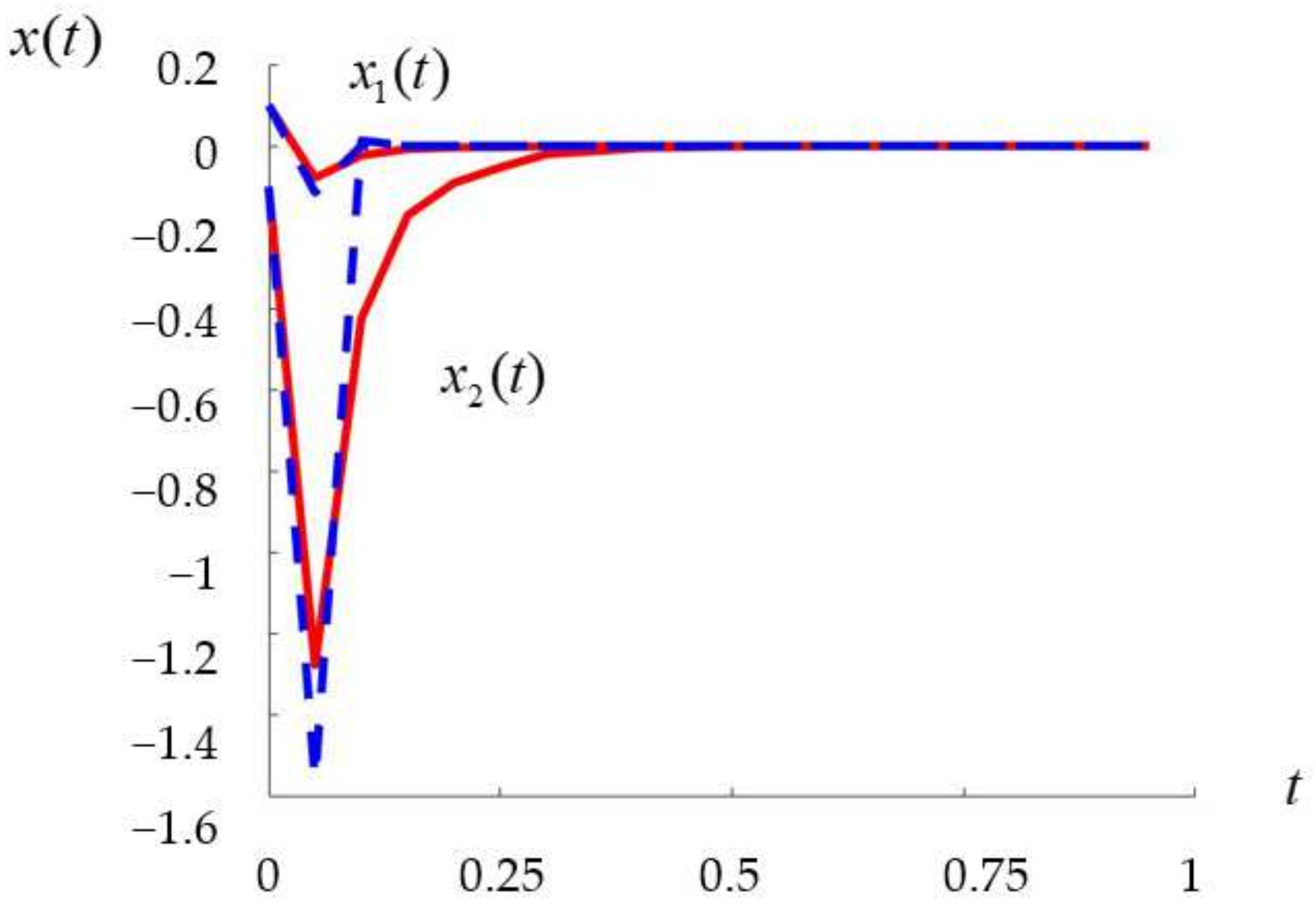
4. Computational Experiments

One of the ways to concretize the coefficients of the system of linear equations for the Padé approximation can be associated with the analysis of the coefficients of the system, and the assumption that the Padé structures form a certain framework, within which the coefficients can be improved from the point of view of the optimality criterion of the control problem. This approach is illustrated below on an example of a simple pendulum [25].

$$\begin{array}{l}t\in \left[0,1\right], \epsilon =0.05, N=20,\\ A(x)=\left(\begin{array}{cc}1& 0.01\\ \frac{-10\sin (x_1)}{x_1}& 1\end{array}\right), B(x)=\left(\begin{array}{c}0.1\\ 0.1\end{array}\right), A_0=\left(\begin{array}{cc}1& 0.01\\ -10& 1\end{array}\right),A_1(x)=1/\epsilon \left(\begin{array}{cc}0& 0\\ \frac{-10\sin (x_1)}{x_1}+10& 0\end{array}\right)\\ x_0={[0.1;-0.1]}^T\\ Q_0=\left(\begin{array}{cc}10& 0\\ 0& 0.05\end{array}\right), Q_1=\left(\begin{array}{cc}300+x_1^2& 0\\ 0& 300+x_2^2\end{array}\right), Q_2=\left(\begin{array}{cc}0& 0\\ 0& 0\end{array}\right),R=1, F=\left[\begin{array}{cc}300& 0\\ 0& 300\end{array}\right].\end{array}$$

Here, $x_1$ denotes the pendulum angle, and $x_2$ is the angular velocity.

Using this example, taking into account the fulfillment of the conditions for the existence of matrices in the representations (18), we will demonstrate the Algorithm 1 for discrete modified Padé regulator construction and the results of its work.

Algorithm 1: Discrete modified Padé regulator construction.

The terms $P_0,{\tilde{\overline{P}}}_1(x),{\tilde{\overline{P}}}_2(x), {П}_{0}P(\tau )$ are found based on the uniform asymptotic approximation of the second order using formulas (10), (12), and (17). The members of the boundary layer terms of the first and second order, ${\widehat{П}}_{1}P(x,\tau )$ and ${\widehat{П}}_{2}P(x,\tau )$, are found approximately, for example, as matrix exponentials with the unknown decay rates constants. The terms of the modified Padé approximation of the solution of the Riccati equation are found from the following system of equations with unknown parameters ${\lambda }_1,{\lambda }_2,{\lambda }_3,{\lambda }_4,{\lambda }_5,{\lambda }_6$ which are the scalar multipliers of the asymptotic expansion terms and are selected using the quality criterion optimization. $$\left(\begin{array}{cccc}E& 0& -{\lambda }_5{\overline{P}}_0& 0\\ 0& E& -{\lambda }_6{П}_{0}P& 0\\ 0& 0& {\lambda }_1{\tilde{\overline{P}}}_1(x)& {\lambda }_2{\overline{P}}_0\\ 0& 0& {\lambda }_3{\widehat{П}}_{1}P(x,\tau )& {\lambda }_4{П}_{0}P(\tau )\end{array}\right)\left(\begin{array}{c}{\mathrm{M}}_1(x)\\ П{\mathrm{M}}_1(x,\tau )\\ {{\rm N}}_1(x)\\ {{\rm N}}_2(x)\end{array}\right)=\left(\begin{array}{c}{\tilde{\overline{P}}}_1(x)\\ 0\\ -{\tilde{\overline{P}}}_2(x)\\ -{\widehat{П}}_{2}P(x,\tau )\end{array}\right).$$ The introduction of multipliers allows us to correct the PA system matrix coefficients within the obtained structure. Such a technique can be used as a basis for the correction of the resulting Padé regulator if the result by the optimality criterion is better than the corresponding results along the regulators using only the asymptotics and regulators built based on the SDRE technique, which is demonstrated in the calculations given below. A regulator built based on this approach will be called a modified Padé regulator. The resultant modified Padé regulator gain is found from (23).

In

Table 1. Regulators comparison by criterion values for $\epsilon =0.05$.

D-SDRE	Uniform First-Order Asymptotic Approximation	Modified Padé [1/2] Approximation
19.2226	16.3533	16.0882089921279

, the criterion values for the regulators based on the uniform first-order asymptotic approximation ($P_0,{\tilde{\overline{P}}}_1(x), {\mathrm{M}}_{0}P(\tau ), {\widetilde{П}}_{1}P(x,\tau )$) and the modified Padé [1/2] from (22) are presented. The comparison is made with the D-SDRE regulator which uses the solution of Equation (9) by the algorithm from [5].

Table 2. Demonstration of extrapolation properties of the modified Padé regulator.

$\mathbf{Parameter} \mathit{\epsilon }$	Modified Padé [1/2] Approximation	Uniform First-Order Asymptotic Approximation	D-SDRE
0.05	16.0882	16.3533	19.2226
0.1	31.7171	29.2683	38.2234
0.125	36.1462	38.6610	47.7203
0.2	64.6920	1630.8255	76.2066
0.25	76.3028	2576.7654	95.1958

shows that the modified Padé [1/2] regulator is closer to the D-SDRE solution by optimality criterion values on a larger interval of parameter variation in comparison with the regulator based on the uniform first-order asymptotic expansion, i.e., demonstrates good quality approximation for larger values of the parameter and has better extrapolation properties. In this example, the uniform first-order asymptotic approximation works only for small parameter values and fails to stabilize the system when the value of the parameter increases. Moreover, the Padé regulator is significantly better by criterion value than the D-SDRE regulator. Thus, here the modified Padé regulator is sufficiently better by optimality criterion than the two other control algorithms (D-SDRE, asymptotic approximation) in the selected parameter variation interval from 0.05 to 0.25 and the asymptotic approximation has a restricted area of application and provides worse quality of the approximation.

The corresponding closed-loop trajectories are presented in Figure 1. It can be seen that the Modified Padé [1/2] approximation brings the system to the neighborhood of the zero-equilibrium point and the trajectories are similar to the D-SDRE solution.

5. Conclusions

Using the SDRE approach, the asymptotics of the solution of the corresponding initial singularly perturbed control problem for the matrix discrete Riccati equation with coefficients weakly dependent on the state is constructed and the corresponding one-point PA regulator is proposed, i.e., only one asymptotic approximation of the Riccati equation solution is used to construct the PA for the feedback gain matrix of the regulator. The results of numerical experiments illustrate, in particular, the improved extrapolation properties of the constructed regulator, which makes the algorithm applicable in control systems for a wider range of parameter variation. An approach for modified PA construction is also demonstrated, which consists of the correction of the system of equations for finding the PA coefficients taking into account the structure of the matrix of the original system and the properties of the terms of the asymptotic approximation.

References

1. Mracek, C.P.; Cloutier, J.R. Control designs for the non-linear benchmark problem via the state-dependent Riccati equation method. Int. J. Rob. Nonlin. Contr. 1998, 8, 401–433. [Google Scholar] [CrossRef]
2. Cimen, T. State dependent Riccati Equation (SDRE) control: A Survey. In Proceedings of the 17th the International Federation of Automatic Control World Congress, Seoul, Korea, 6–11 July 2008; Volume 41, pp. 3761–3775. [Google Scholar]
3. Dmitriev, M.G.; Makarov, D.A. Smooth nonlinear controller in a weakly nonlinear control system with state depended coefficients. Trud. ISA RAN 2014, 64, 53–58. (In Russian) [Google Scholar]
4. Chang, I.; Bentsman, J. Constrained discrete-time state-dependent Riccati equation technique: A model predictive control approach. In Proceedings of the 52nd IEEE Conference on Decision and Control, Florence, Italy, 10–13 December 2013; pp. 5125–5130. [Google Scholar]
5. Dutka, A.S.; Ordys, A.W.; Grimble, M.J. Optimized discrete-time state dependent Riccati equation regulator. In Proceedings of the American Control Conference, Portland, OR, USA, 8–10 June 2005; pp. 2293–2298. [Google Scholar]
6. György, K.; Dávid, L.; Kelemen, A. Theoretical Study of the Nonlinear Control Algorithms with Continuous and Discrete-Time State Dependent Riccati Equation. Procedia Technol. 2016, 22, 582–591. [Google Scholar] [CrossRef] [Green Version]
7. Danik, Y.E.; Dmitriev, M.G. The robustness of the stabilizing regulator for quasilinear discrete systems with state dependent coefficients. In Proceedings of the International Siberian Conference on Control and Communications, Moscow, Russia, 12–14 May 2016. [Google Scholar]
8. Emel’yanov, S.V.; Danik, Y.E.; Dmitriev, M.G.; Makarov, D.A. Stabilization of nonlinear discrete-time dynamic control systems with a parameter and state dependent coefficients. Dokl. Mathem. 2016, 93, 121–123. [Google Scholar] [CrossRef]
9. Danik, Y.E.; Dmitriev, M.G. The comparison of numerical algorithms for discrete-time state dependent coefficients control systems. In Proceedings of the 21st International Conference on System Theory, Control and Computing, Sinaia, Romania, 19–21 October 2017; pp. 401–406. [Google Scholar]
10. Danik, Y.E.; Dmitriev, M.G. Construction of Parametric Regulators for Nonlinear Control Systems Based on the Padé Approximations of the Matrix Riccati Equation Solution. In Proceedings of the 17th the International Federation of Automatic Control Workshop on Control Applications of Optimization, Yekaterinburg, Russia, 15–19 October 2018; Volume 51, pp. 815–820. [Google Scholar]
11. Danik, Y.E.; Dmitriev, M.G. The construction of stabilizing regulators sets for nonlinear control systems with the help of Padé approximations. In Nonlinear Dynamics of Discrete and Continuous Systems; Abramian, A., Andrianov, I., Gaiko, V., Eds.; Springer: Cham, Switzerland, 2021; pp. 45–62. [Google Scholar]
12. Heydari, A.; Balakrishnan, S.N. Approximate closed-form solutions to finite-horizon optimal control of nonlinear systems. In Proceedings of the American Control Conference, Montreal, QC, Canada, 27–29 June 2012; pp. 2657–2662. [Google Scholar]
13. Kvakernaak, H.; Sivan, R. Linear Optimum Control Systems; Wiley-Interscience: New York, NY, USA, 1972. [Google Scholar]
14. Vasil’eva, A.B.; Butuzov, V.F. Asymptotic Expansions of a Solutions of Singularly Perturbed Equations; Nauka: Moscow, Russia, 1973. (In Russian) [Google Scholar]
15. Vasil’eva, A.B.; Butuzov, V.F.; Kalachev, L.V. The Boundary Function Method for Singular Perturbation Problems; Society for Industrial and Applied Mathematics: University City, MO, USA; Philadelphia, PA, USA, 1995. [Google Scholar]
16. Vasil’eva, A.B.; Dmitriev, M.G. Singular perturbations in optimal control problems. J. Sov. Mathem. 1986, 34, 1579–1629. [Google Scholar] [CrossRef]
17. Kurina, G.A.; Dmitriev, M.G.; Naidu, D.S. Discrete singularly perturbed control problems (A survey). Dyn. Contin. Discr. Impuls. Syst. Ser. B Appl. Algor. 2017, 24, 335–370. [Google Scholar]
18. Glizer, V.Y.; Dmitriev, M.G. Asymptotics of a solution of some discrete optimal control problems with small step. Different. Equat. 1979, 15, 1681–1691. (In Russian) [Google Scholar]
19. Gaipov, M.A. Asymptotics of the solution of a nonlinear discrete optimal control problem with small step without constraints on the control (formalism). I. Izvest. Akad. Nauk TurkmenSSR 1990, 1, 9–16. (In Russian) [Google Scholar]
20. Belokopytov, S.V.; Dmitriev, M.G. Direct scheme in optimal control problems with fast and slow motions. Syst. Contr. Lett. 1986, 8, 129–135. [Google Scholar] [CrossRef]
21. Afanas’ev, V.N. Control of nonlinear plants with state-dependent coefficients. Autom. Remote Control 2011, 72, 713–726. [Google Scholar] [CrossRef]
22. Afanas’ev, V.N.; Presnova, A.P. Parametric Optimization of Nonlinear Systems Represented by Models Using the Extended Linearization Method. Autom. Remote Control 2021, 82, 245–263. [Google Scholar] [CrossRef]
23. Baker, G.A.; Baker, G.A., Jr.; Baker, G.; Graves-Morris, P.; Baker, S.S. Padé Approximants: Encyclopedia of Mathematics and It’s Applications, 2nd ed.; Cambridge University Press: Cambridge, UK, 1996. [Google Scholar]
24. Balandin, D.; Kogan, M. Synthesis of Control Laws Based on Linear Matrix Inequalities; Fizmatlit: Moscow, Russia, 2007. (In Russian) [Google Scholar]
25. ElBsat, M.N. Finite-Time Control and Estimation of Nonlinear Systems with Disturbance Attenuation. Ph.D. Thesis, Marquette University, Milwaukee, WI, USA, August 2012. [Google Scholar]
Figure 1. Closed-loop system trajectories: Modified Padé [1/2] approximation (red lines) and D-SDRE (blue lines).
Mathematics 10 00487 g001