Abstract
In optimization, algorithm selection, which is the selection of the most suitable algorithm for a specific problem, is of great importance, as algorithm performance is heavily dependent on the problem being solved. However, when using machine learning for algorithm selection, the performance of the algorithm selection model depends on the data used to train and test the model, and existing optimization benchmarks only provide a limited amount of data. To help with this problem, artificial problem generation has been shown to be a useful tool for augmenting existing benchmark problems. In this paper, we are interested in the problem of knowledge transfer between the artificially generated and existing handmade benchmark problems in the domain of continuous numerical optimization. That is, can an algorithm selection model trained purely on artificially generated problems correctly provide algorithm recommendations for existing handmade problems. We show that such a model produces low-quality results, and we also provide explanations about how the algorithm selection model works and show the differences between the problem data sets in order to explain the model’s performance.
1. Introduction
In optimization, automated algorithm selection is the task of selecting an algorithm that is best suited to solving a specific problem [1]. This is an important task, as different optimization problems are best solved by different algorithms, and there is no single algorithm that performs well across all possible problems [2].
When an automated selection model is used to predict the best performing algorithm on a new problem, it is important that the prediction model has been trained on a large number of problems similar to the new problem. However, as the number of handmade benchmark problems is limited, acquiring training data for a large number of different problems is difficult. To help solve this problem, recent research has shown that artificial problem generation techniques can be used to augment existing optimization benchmark sets with additional problems.
In this paper, we are interested in transfer learning—seeing how a model trained on a set of artificially generated benchmark problems performs when it is used to predict the performance of optimization algorithms on a set of handmade benchmark problems. To determine this, we examine the performance of a machine-learning-based algorithm selection model on two different continuous optimization problem sets. The first is an artificial problem set created by a problem generator developed by Tian et al. [3]. The second is a handmade problem set used by the well known Comparing Continuous Optimizers (COCO) benchmarking platform [4]. We first analyze how an algorithm selection model behaves when trained and tested on each of these two problem sets individually. We then examine the model’s performance when trained and tested on a combined problem set containing both artificial and handmade benchmark problems. Finally, we focus on determining the possibility of transfer learning by examining how a model trained on one of these problem sets performs when tested on the other.
To accomplish this, we use exploratory landscape analysis (ELA), a methodology that transforms problem samples into numerical descriptors of the underlying problem called landscape features. ELA was first introduced by Mersmann et al. in [5] and later expanded in [6]. Since its introduction, it has been used for a variety of different applications, including algorithm selection [7].
To explain the results of the algorithm selection model, we also perform two different experiments that analyze both the optimization problems as well as the algorithm selection models. The different problems sets are examined using correlation analysis to determine the similarities of the problems between the two problem sets. The decision making of the algorithm selection models is analyzed using the Shapley Additive Explanations (SHAP) framework [8], which explains for every prediction which features contributed to that prediction and by how much. This allows us to examine which landscape features are important for classifying the problems from the two problem sets, and if the important features differ between the two sets. If the features differ between the sets, this indicates that there are large differences in the problems that make transfer learning difficult. It might also indicate that the landscape features themselves have difficulties generalizing between different types of problems.
The rest of this paper is structured in the following way. Section 2 gives an overview of related work. Section 3 gives an overview of the methodology used in our analysis. Section 4 presents the results of our analysis. Section 5 discusses the implication of our results. Finally, Section 6 summarizes our findings and lists ideas for future work.
2. Related Work
In the field of optimization, automated algorithm selection is a popular area of research as optimization algorithm performance is heavily dependent on the problem being solved [9]. One example of this is Kerschke et al. [7], which presents both a regression and a classification based algorithm selection approach, and evaluates it on the COCO problem set. Using this approach to automatically select algorithms for each specific problem reduced the estimated runtime of the system by half compared to only using a single algorithm. Another example is presented by Jankovic et al. [10], which uses trajectory-based sampling instead of calculating ELA with random samples. Most of the referenced algorithm selection approaches use ELA-based regression to predict the performance of each algorithm, and then select the best performing one [9,10,11,12,13,14,15]. In our experiments, we instead use multi-class classification to simply select the best performing algorithm.
However, these algorithm selection experiments have focused on only a single problem set, using its problems as both training and testing data. Transfer learning, the task of training a model on one dataset and using to predict a different set, is a popular topic of research in machine learning. Zhuang et al. present a comprehensive survey of the current state of the art in [16]. While transfer learning is popular in fields such as bioinformatics, natural language processing, and transport systems, it has to our knowledge not been thoroughly explored in the context of optimization algorithm selection. In [17], Lacroix and McCall show poor results when using transfer learning between COCO problems and artificially generated Interpolated Continuous Optimisation Problems (ICOP problems). However, the case-based reasoning performed poorly even when trained and evaluated solely on the ICOP problems. This makes assessment of the performance of the transfer learning a harder task in this specific case.
One way of further improving algorithm selection which can be applied to transfer learning is the use of artificially generated problems to augment existing handmade benchmark sets. Muñoz and Smith-Miles have shown that ELA features can be used to augment the existing COCO problem set [18]. Lacroix et al. [19] introduce a class of artificially generated problems called ICOP and show that they can be optimized to produce difficult problems according to three different metrics. In addition to generating problems, Fisbach and Bartz-Beielstein have shown a methodology for selecting a good subset from a large number of generated problems in order to improve reliability and generalizability of problem generators [20].
3. Methodology
In this section, we present the overview of the methodology used in this paper. Our methodology is split into three parts: problem portfolio representation, supervised machine learning, and the complementarity analysis which uses correlation and Shapley analysis to provide more explainable results.
In the problem portfolio representation part, we introduce the datasets used for training and testing the automated algorithm selection model with one set containing artificially generated problems and the other containing handmade benchmark problems. We then create the problem portfolio representation by calculating the exploratory landscape features that will be used as training attributes in the supervised machine learning part of our methodology.
In the supervised machine learning part, we examine the performance of a machine-learning-based algorithm selection model on the two problem sets introduced in the portfolio representation part. In particular, we are interested in seeing how an algorithm selection model trained on a set of artificially generated problems behaves when tested on the set of handmade benchmark problems. This part forms the main contribution of this paper.
In the complementarity analysis part, we further examine the complementarity of the artificially generated problem set with the handmade problem set by using visualization and correlation comparison techniques, using the methodologies from [21,22].
3.1. Problem Portfolio Representation
The first step of our methodology involves generating an artificial benchmark problem set, selecting the handmade problems that we will use for our comparison, and calculating exploratory landscape features.
The artificial problems set is generated using the generator described by Tian et al. in [3]. The generator works by representing optimization problem as a tree, which is randomly extended using a fixed set of operators. In addition to traditional mathematical operators such as multiplication and division, the generator also uses 8 different difficulty injection operations which are designed to introduce problems commonly encountered in real-life problems, such as adding noise or introducing multimodality. After the tree is grown to a predefined size, it is converted into a reverse polish notation so that it can be more easily evaluated.
The problem generator assigns each generated problem a single best performing algorithm. The best performing algorithm is determined by running 10 optimization algorithms on the problem and selecting the best performing one. Table 1 lists the 10 algorithms used. The parameters used for the algorithms are unchanged from the initial settings of the problem generator. Table 2 lists the parameters used for each algorithm. Other than the population size, which is set at 100 for every algorithm, the parameters use default values from the literature in which they were introduced. Each algorithm is evaluated using 20 independent runs, and the mean of the minimum objective value is used as the performance metric. The termination condition of each run is set at 10,000 function evaluations. A brief description of the algorithms used is provided below.

Table 1.
The Algorithms used by the artificial problem generator.

Table 2.
The parameters used by the algorithms of the artificial problem generator.
Artificial Bee Colonyis a swarm optimization algorithm inspired by the behaviour of bees that splits its population into three types: scouts, onlookers, and employed bees. The scout bees provide the algorithm with exploration power, while the other two types provide exploitation power.
Ant Colony Optimization is a swarm optimization algorithm inspired by the behaviour of ants. As individuals of the population explore the subspace, they leave behind an artificial pheromone that guides other individuals in their own exploration.
Differential Evolution is an evolutionary algorithm that starts with a randomly initialized population, which is improved every generation using crossover and mutation operators.
Fast Evolutionary Programming is a modification of a traditional evolutionary algorithm that uses the Cauchy rather than the Gaussian distribution for the mutation operator in order to improve the speed of convergence.
Genetic Algorithm is a traditional genetic algorithm. While genetic algorithms were initially designed to solve combinatorial problems, the implementation used by the artificial generator uses a methodology that simulates binary crossover for continuous domains.
Particle Swarm Optimization is a swarm optimization algorithm where the movement of each particle is determined by his own best known position, as well as the global best known position.
Competitive Swarm Optimizer is a modified Particle Swarm Optimization algorithm where the particles are no longer updated based on best known positions, but by a competition system that pairs two particles together, with the losing particle (the particle with the lower fitness) updating its position based on the winning particle (the particle with the higher fitness).
Simulated annealing uses population of solutions where each member examines a random point in its neighbourhood, and either stays in his current position or switches to the new point based on the evaluation of the new point as well as on a probability function. The probability of swapping changes during the optimization.
Random Search simply assigns each member of the population a random position in each iteration.
Covariance matrix adaptation evolution strategy is an optimization method similar to quasi-Newtonian methods that aim to approximate the second-order derivative matrix of the underlying problem. Unlike the quasi-Newtonian methods, it does not use gradients, which makes it usable on a larger amount of problems.
After the mean objective values are computed for each of the 10 algorithms, a Wilcoxon sum-rank test is performed to determine if there are any algorithms for which there is no statistically significant difference in performance when compared to the best performing algorithm. If such algorithms exist, the generated problem is discarded. This ensures that for every generated problem, there is only a single best performing algorithm from a statistical point of view.
The handmade benchmark problem set consists of the problems from the COCO optimization platform [4], specifically from its noise-free single-objective benchmark set. This benchmark set was chosen because it is a well known and widely used set of benchmark problems in the optimization community, and is also the problem set used by a large number of existing works on exploratory landscape analysis. This set of problems is structured in the following way. It contains 24 unique base problems, with each of these base problems being further split into a large number of instances. These instances are created by transforming the base problem using shifting and/or scaling. As these instances are created programmatically by applying a transformation to the base problem, there is technically an unlimited number of instances available. In our experiments, we will use the first 15 instances of each of the 24 base problems, for a total of 360 instances.
We will refer to the 24 base problems as the base COCO problems, and the individual instances as COCO instances.
We determine the best performing algorithms on the COCO instances using the same procedure with the same set of 10 optimization algorithms as used for the artificial instances. A large difference between the COCO and the artificial instances is that for the COCO instances, it is possible that multiple algorithms are statistically tied as the best performing algorithm. Specifically, only 140 out of 360 instances contain a single best performing algorithm, while 220 instances contain multiple algorithms for which there is no statistical difference in performance when compared to the best performing algorithm.
We deliberately chose to not modify the original artificial problem generator so that it would not discard instances where there was no statistical difference in the performance of multiple algorithms. This was done because we wanted to limit the scope of this paper to only use the original problem generator exactly as described in [3] without any modification and because we did not want to modify the artificial problem generation procedure using the knowledge of the COCO problem set. We also chose to use the entire set of 360 COCO instances, rather than just the set of 140 instances that contain a single best performing algorithm, as we did not want to tailor the composition of the COCO set based on the knowledge of how the artificial set was constructed.
This difference in the performance of the algorithms indicates a potentially large difference between the instances of the artificial and the COCO sets. We can see that the artificial set only contains a relatively small subset of all possible instances that could be generated, as only the 30% of the instances with a single best performing algorithm are kept. On the other hand, the majority of COCO instances have multiple algorithms for which there is no statistical difference in performance. Because of this, the only potential for overlap between the two problem sets are the 140 COCO instances that are only solved well by a single algorithm.
In total, our final machine learning dataset contains 500 artificial instances, 50 for each class, as well as 360 COCO instances. For both the artificial and the COCO instances, we collect instance samples. These samples are then used to calculate exploratory landscape features, which are used as a basis for all following experiments.
3.2. Machine Learning
In the second part of our methodology, we train and evaluate an algorithm selection model to determine the best performing algorithm on each instance, using the exploratory landscape feature representations introduced in the previous section and the random forest machine learning algorithm [34].
The dataset used for machine learning consists of exploratory landscape features for the attributes, and the best performing algorithm on the specific instance as the prediction class. Each data row represents a single optimization instance. To account for the COCO instances that contain multiple algorithms for which there is no statistical difference in performance, two types of machine learning experiments are performed. In the first, only the single absolute best performing algorithm is used as a prediction class. In the second, the prediction of the model is considered correct if any of the algorithms for which there is no statistical difference compared to the absolute best performing algorithm is predicted. The second type mirrors a practical application of algorithm selection, where we are not interested in finding all possible algorithms that solve a particular problem well, and are instead satisfied with finding a single well performing algorithm.
In order to evaluate machine learning performance, we conduct several experiments that differ in the data used for the training and the testing sets. These experiments are:
- COCO (Instance Split)—The model is trained on the COCO instances and tested on the COCO instances, using instance based stratified cross validation. Here, the training data contains 14 instances of each of the 24 base problems, and the testing data contains the final 15th instance of each base problem. This means the model can learn from all of the 24 base problems.
- COCO (Problem Split)—The model is trained on the COCO instances and tested on the COCO instances, using problem based stratified cross validation. Here, the training data contains all 15 instances of 23 base problems, and the testing data contains the 15 instances of the final 24th base problem. This means the model only learns on 23 base problems and then predicts the final 24th base problem.
- Artificial—The model is trained on the artificial instances and tested on the artificial instances. Since the artificial set cannot be split by base problems, we split the training and testing sets randomly using cross validation.
- Combined—The model is trained on a combined set of both artificial and COCO instances, and tested on the combined set of instances. Cross validation is used to split the training and testing set.
- Transfer—The model trained on the artificial instance, and tested on the COCO instances. The full artificial set is used for training, and the full COCO set is used for testing.
In the first three experiments, we are interested in seeing how the algorithm selection model performs on both of the problem sets in isolation, to obtain a baseline performance metric. In the final two experiments, we focus on the main task of this paper, first by combining the two problem sets, and finally by examining the effectiveness of transfer learning between artificial instances and COCO instances.
In case of the COCO problem set, we split the evaluation into two cases. In the first case (instance split), the training data contains similar instances to the testing data, as instances represent variations of the original base problem and all 24 base problems are used for both training and testing. We expect this to produce good results, as the training data contains information about all of the COCO base problems. In the second case (problem split), the training data contains no information about the base problem in the testing set. We expect this to produce poorer results, as the training set contains no information about the base problem used for the testing data. This case can be considered a type of transfer learning, as the training data contains information that is entirely different from the testing set.
For the artificial case, the model is trained and tested on the instances from the artificial set, with 10-fold cross validation used to achieve more reliable results. In the combined case, both the artificial and the COCO instances are combined into a single set that is then used for both training and testing, also using 10-fold cross validation. Finally, in the transfer case, the model is trained on the artificial instances, and then tested on the COCO instances. Here, no cross validation is used, as we already use different sets for training and testing. However, since we use the random forest algorithm to perform machine learning, we repeat this experiment 10 times and use mean values of the performance metrics to obtain more reliable results.
3.3. Complementarity Analysis
The final part of our methodology focuses on gaining a deeper understanding of the machine learning results obtained in the previous section.
First, we examine the hand-made and the artificially generated problems by performing correlation analysis as described in [21]. This allows us to directly examine the correlations between the individual instances. Ideally, instances that are solved well by the same algorithm should be correlated with each other.
Second, we examine the algorithm selection models using a methodology called SHapley Additive exPlanations (SHAP) [8]. This methodology assigns to every landscape feature of a particular instance a value that describes how much this landscape feature contributed to the selection model’s decision to classify this instance as a particular class. This allows us to determine which landscape features most contribute to the classification of every individual class.
4. Results
In this section, we present the results of the experiments presented in Section 3.
4.1. Problem Selection and Feature Calculation
Before proceeding with the artificial problem generation, we first wanted to verify that the algorithm generation procedure would produce the same distribution of problems as the one described in [3], even when using a smaller sample size. As the process of calculating exploratory landscape features is time consuming, we had to use a smaller number of problems than used in [3], where exploratory landscape analysis was not used. Because of this we first wanted to ensure that a smaller number of problems would not introduce additional bias. The artificial problem generation works as described in [3], using the source code that was made available online (The source code is available at https://github.com/BIMK/Algorithm-Recommendation, (accessed on 30 December 2021)) by the authors of the paper, using a dimensionality of .
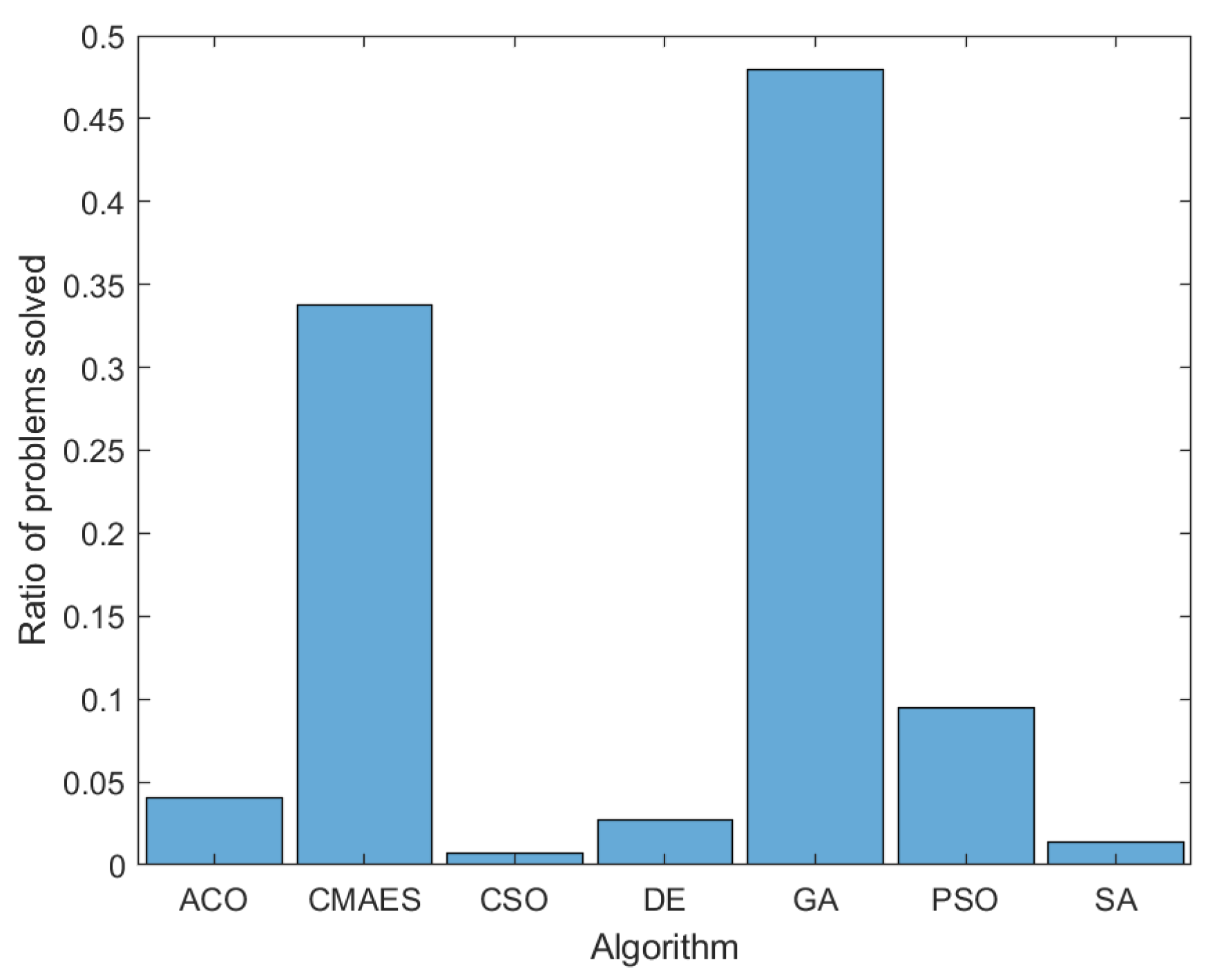
Figure 1 shows an example distribution of 500 problems generated in a single run, based on which optimization algorithm best solved the generated problems, using the algorithms and algorithm parameters described in [3]. We can see that this distribution broadly matches the one in the original algorithm generation paper, with GA [28,29] and CMA-ES [33] algorithms solving the majority of the generated problems.
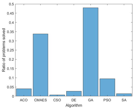
Figure 1.
A sample distribution of generated problems, based on which optimization algorithm best solves the generated problem.
For a more thorough evaluation, we conducted a statistical analysis where different sample sizes were tested based on the algorithm frequency of solved problems, as we wanted to find the smallest number of problems to generate that would preserve the problem distribution from [3]. We generated multiple different sets of problems, with the number of problems (i.e., sample size) in {500, 1000, 5000, 10,000}. For each sample size we repeated the sampling 10 times. Then, the samples were compared using the information of how many problems were solved by each of the 10 algorithms. For this purpose, we used the Friedman test, since we were comparing more than 2 samples and the required conditions for the safe use of the parametric tests have not been satisfied. For comparisons between different sample sizes all their samples were compared, for a total of 20 samples, 10 for each sample size. Table 3 shows the p-values obtained for the comparisons. We can see that all p-values are above the critical value of , and thus there is no statistically significant difference between the samples regardless of the sample size used.

Table 3.
p-values of the Friedman test used to determine whether multiple runs of the problem generation algorithm produce the same distribution of problems depending on the number of problems used.
4.2. Machine Learning
For the machine learning analysis, we create two separate datasets. The first consists of the artificial benchmark instances, while the second consists of handmade COCO instances. The artificial problem set contains 500 generated instances, with 50 instances from each of the 10 different prediction classes (algorithms that best solve the problem). This was done in order to create a balanced machine learning dataset. The COCO problem set contains 15 instances for each of 24 base problems, for a total of 360 instances.
To obtain a more robust set of features, each instance is sampled separately 10 different times, using latin hypercube sampling with a sample size of , the dimensionality D of 10, and taking samples from the range of . A single dimensionality of 10 was chosen because it offers a balance between problem complexity and computational costs. As the complexity of calculating some landscape features raises polynomially or even exponentially with regards to the dimensionality and the number of samples, higher dimensionalities are much harder to compute. We calculate the exploratory landscape features separately for each of these samplings, creating 10 different sets of landscape features for each problem. The median of these 10 sets is used as the final set of landscape features. The use of medians to obtain a more robust set of features has been used for example in [10,15].
The landscape features were calculated using the R library flacco [35], a widely used open source R library that collects a large amount of different ELA techniques proposed by multiple authors in a single library, and allows users to calculate them with a single function call. We used the landscape feature categories cm_angle, cm_grad, ela_level, ela_meta, ic, disp, limo, nbc, and pca. A detailed overview of these features is presented in [35]. This excludes some flacco feature categories, particularly those that are either computationally expensive in higher dimensions or require an exact problem definition to be known and additional sampling to compute.
Some of the landscape features produced errors or resulted in NA values when computed on certain artificially generated instances. As the number of instances is limited, we chose to remove these landscape features from our final machine learning dataset to ensure that all of the artificial instances could be used for the machine learning data. The full list of 50 landscape features used is listed in Table 4.

Table 4.
All landscape features used as machine learning attributes, with the names taken from the flacco library.
All machine learning is performed using the random forest [34] algorithm, as this algorithm has been shown to perform well when predicting algorithm performance using the COCO dataset [7]. The random forest algorithm is an upgrade to the traditional decision tree. Decision trees build their model by creating a tree which starts at a root node, and then splits the dataset according to a single attribute in each node. However, such models often overfit the training data if techniques such as pruning are not used [36]. The random forest algorithm improves on this shortcoming by using an ensemble of simple decision trees, with each tree using only a randomly selected subset of all available attributes in each split and a random sample of all available instances in each tree. Similar to bootstrap sampling, this decreases the variance of the model without increasing its bias. We use the R library randomForest [37] which provides an implementation of the algorithm in the R programming language. The parameter (number of trees) is set to 1000, and using the default parameters values for all other parameters. The number of trees was determined experimentally. Generally speaking, increasing the number of trees increases the performance of the algorithm but requires additional computational time. However, past a certain point additional trees no longer produce a difference in performance. We determined that increasing the number of trees past 1000 did not produce any improvement in results. The full parameters used are listed in Table 5.

Table 5.
Full list of parameters used for the random forest algorithm. Other than the number of trees which is set to 1000, all other parameters use default values. The left side lists the parameter name, with the name used in the R code specified in brackets.
The number of sampled variables (mtry) determines how many random attributes are considered for each split. The square root of the number of classes is a typical default value [38] for classification. The sampling with replacement parameter determines if the instances sampled for each decision tree should be done with replacement or without. Sampling with replacement is generally done, as it reduces the variance of the model without increasing its bias, in the same way as bootstrap sampling. The cutoff parameter determines how the ensemble of trees selects a single winner, and essentially allows us to specify weights for each of the prediction classes so that certain classes require a higher number of votes to be selected. Leaving this parameter at assigns equal weights to all classes. Finally, the minimum size of terminal nodes and the maximum number of terminal nodes can be used to limit the size of the generated trees, resulting in faster performance at the expense of limiting the types of trees that the model can create. The default values of 1 and unlimited put no limits on the types of trees that can be generated, and are used as our dataset is small enough that it does not require the additional performance benefits of smaller trees.
Additionally, we chose to use the default parameters because we are not interested in achieving optimal machine learning results, but rather in comparing the relative difference in performance when using different training and testing datasets. The number of trees was chosen experimentally, as we determined that increasing the number of trees further did not result in a large performance increase.
Before analyzing the results of the automated algorithm selection model, we will first more closely examine the data used to make the predictions. Table 6 shows which algorithms achieved the absolute best optimization result for every COCO base problem. However, each base problem contains 15 distinct instances, and these instances can be solved best by different optimization algorithms. Because of this, the table can show several algorithms as the best performing algorithm for each base problem. This might occur due to slight differences in the instances. Another reason might be the stochastic nature of the optimization algorithms, with multiple runs on a similar problem producing a different best algorithm.

Table 6.
The algorithms that best solved each individual COCO base problem. In some cases, certain COCO instances belonging to the base problem were solved by a different algorithm. For the problems where this occurred, the other algorithms are listed in brackets.
Table 7 shows the accuracy, as well as the macro precision and recall scores for the five algorithm selection models described in Section 3 when all landscape features were used and only the single best performing algorithm was used as a classification target for the COCO instances.

Table 7.
The results of the algorithm selection model trained using every available landscape feature.
The macro precision and recall metrics are calculated by taking the average of the per-class precision and recall. In some cases, it is possible for the precision and recall to be undefined for some classes. Precision is undefined if both true positives and false positives equal 0 (i.e., no instance in the testing set was classified with a specific class). Recall is undefined if both true positives and false negatives are 0 (i.e., there is no instance of a specific class in the testing set). If the values for precision or recall are undefined for a specific class, this class is not used when calculating the macro metrics.
In the experiments where cross fold validation is used, the final precision and recall metrics are the average values across all folds. In the transfer case, when no cross fold validation is used but the experiments are repeated 10 times to achieve more robust results, the average of the 10 runs is used.
We can see that the choice of the train-test split has a large effect on the results of the two models trained on COCO data. If the training and testing sets are stratified per instance, the model achieves an accuracy of 0.68. However, if the sets are stratified per problem, the accuracy drops to 0.26. These results show the importance of having similar instances in the training and in the testing set. The artificial and the combined set achieve an accuracy of 0.52 and 0.61 respectively.
Finally, the transfer learning produces poor results, with an accuracy of only 0.20. This indicates that the two problem sets are distinct from one another, and that the instances in the artificial set do not contain enough information about the instances in the COCO set, similar to the results of when the COCO set is stratified per problem. The precision and recall scores likewise produce very poor results.
For a more detailed examination of the transfer learning results, Table 8 shows the confusion matrix of the predictions. We can see that the model’s predictions are heavily concentrated on a few of the classes, specifically CMAES, CSO, and DE.

Table 8.
The confusion matrix for transfer learning, using only all landscape features.
In order to attempt to improve transfer learning accuracy, we used the findings from [22], and limited the machine learning data to only the features that were found invariant to the transforms of shifting and scaling. The results from these experiments are presented in Table 9, and the specific landscape features used are presented in Table 10. Only a set of 13 invariant landscape features is used, as some of the features that were found invariant in [22] were removed from our data as they produced errors when calculated on some of the artificially generated problems. We can see that this produces similar or even slightly better results, which indicates that these 13 features alone contain similar amount of information relevant for classification compared to the full 67 feature set.

Table 9.
The results of the algorithm selection model trained using invariant features.

Table 10.
The list of 13 landscape features that were determined to be invariant to shifting and scaling, with the names taken from the flacco library.
Table 11 shows the confusion matrix of the predictions from transfer learning when using only the invariant features. We can see that the results are similar to the ones obtained when using the full feature set. However, we can see that the predicted classes are now slightly more varied, with more instances being predicted as ABC and ACO.

Table 11.
The confusion matrix for transfer learning, using only the landscape features that were found to be invariant to shifting and scaling. The columns represent true classes, while the rows represent the predictions.
The poor results of the transfer learning experiment could be explained by the single-label setup of the machine learning experiment. Because a large number of the COCO instances have multiple algorithms for which there is no statistical difference in performance, it’s possible that in some cases where the COCO instances are miss-predicted, the algorithm that was predicted wasn’t the absolute best performing, but instead one of the algorithms for which there was no statistical difference in performance.
However, the model achieves poor results even if the COCO problems where multiple algorithms perform well are excluded from the test set and only the 140 COCO instances with a single best performing algorithm are used for evaluation. In this scenario, the accuracy achieved by a transfer learning model increases to 0.30 when using all features and 0.32 when using the features invariant to shifting and scaling.
To further account for this scenario, we conduct the second machine learning experiment where the models tested on the COCO problems were reevaluated by considering all of the algorithms with no statistical difference in performance to the best algorithm as the correct prediction. This creates an experiment that is similar to multi-label classification. However, in our case, the trained model used is still the same as used in the original single-label experiments, and so only a single class can be predicted by the trained model. This separates our experiment from a true multi-label scenario.
Table 12 shows the results of this experiment for the three cases that use the COCO instances as the testing dataset.

Table 12.
The results of the algorithm selection model when considering all algorithms without statistically significant difference to the absolute best performing algorithm to be a correct prediction.
Only accuracy is reported, since per class precision and recall metrics cannot be used with this experimental setup as there are multiple correct labels for each instance, i.e., multiple algorithms for which there is no statistical difference in performance when compared to the best performing algorithm. We present both the variant of the experiment that uses all available landscape features, as well as the variant that uses only landscape features invariant to shifting and scaling. As only a single class is predicted, evaluation metrics used for multi-label classification such as Hamming loss also cannot be used. Because the artificial data set only contains a single correct label, these results do not include the scenario where the model is both trained and tested on the artificial instances. As the scenario where the model is trained and tested on a combined set of problems also includes the artificial instances, we also chose the exclude that scenario.
From the results we can see that this increases prediction accuracy, as was expected. The COCO instance split case now achieves an accuracy of 0.90, predicting most instances correctly. The COCO problem split case now achieves an accuracy of 0.47 up from 0.21, and the transfer learning case achieves an accuracy of 0.40. These results are now close to the results achieved on the model that was both trained and tested on the artificial instances in the previous experiment. However, despite the improvement in the transfer learning cases we can see that both of them achieve an accuracy that is still much lower than the instance split case.
4.3. Complementarity Analysis
After the machine learning part of our methodology, we perform several additional experiments aimed at exploring the complementarity of the artificially generated problem set and the COCO problem set. To improve the result of this analysis, we use Singular Value Decomposition (SVD), as described in [21]. Singular value decomposition is a mathematical procedure which is used in machine learning to transform the original data, represented as a matrix M, into , where is a diagonal matrix which contains singular values on its diagonal. These singular values provide us with a new representation of the data. This is beneficial because the singular values are not linearly correlated with one another. As a large number of the landscape features used in our initial dataset are correlated, transforming them in this way has been shown to improve the quality of the visualization [21]. We perform the SVD projection by first calculating the SVD mapping using the landscape features from the artificial instances, and then projecting the COCO features into the subspace of the artificial features.
As our dataset contains a relatively large amount of data, visualizing all instances would not provide readable visualizations. Instead, we only use a subset of all instances for the analysis in this section. Specifically, we randomly sample the artificial and COCO instances, while preserving the class distribution of the whole set. For the artificial instances, we sample two instances from every class, for a total of 20 instances. For the COCO instances, we sample one instance from each base problem, for a total of 24 instances. This results in 44 sample instances that will be used for the visualization. Because the procedure of sampling the instances is stochastic, we repeat this procedure three times to obtain a three alternative samplings. We use these samplings to show multiple examples of the resulting visualizations.
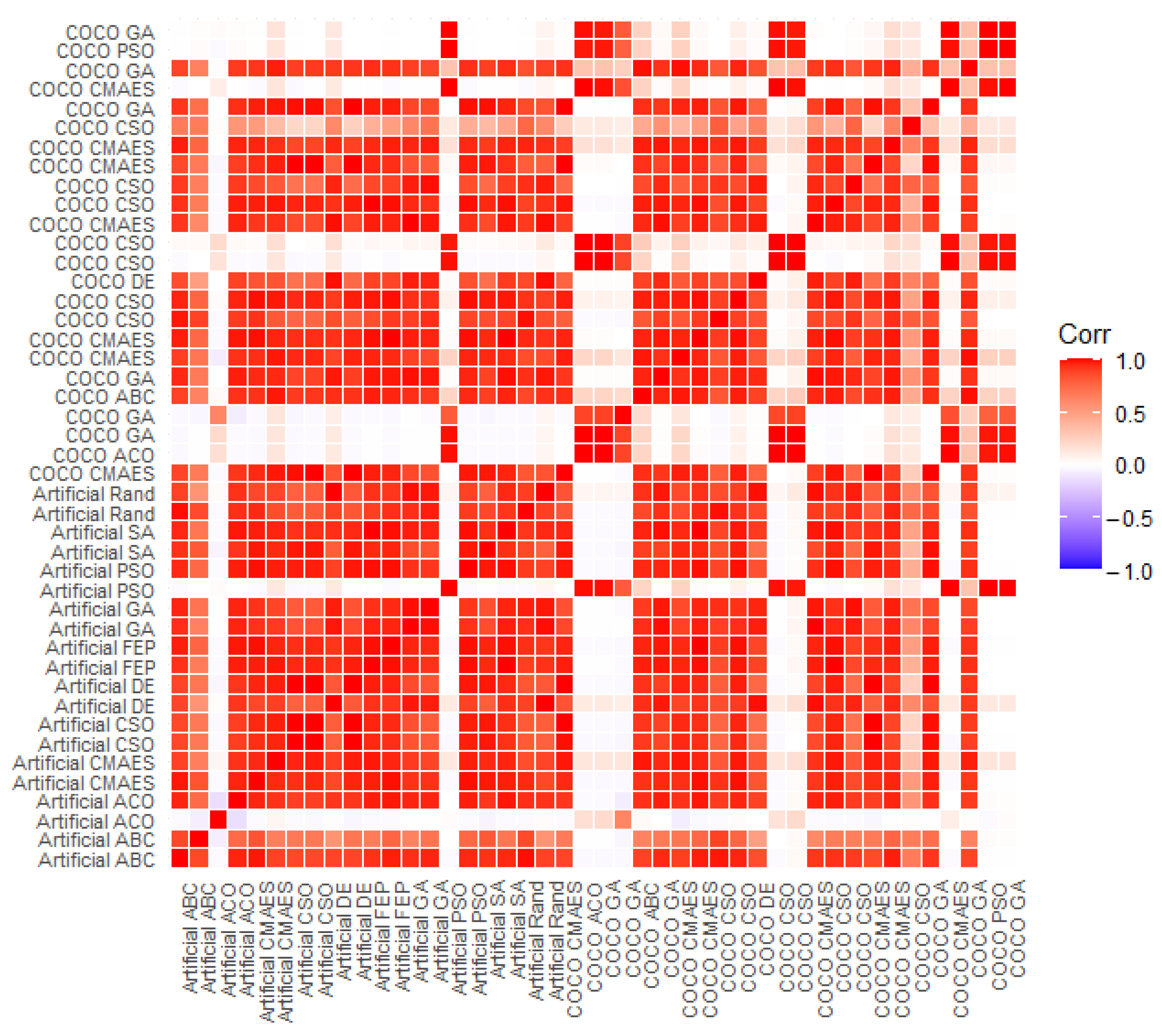
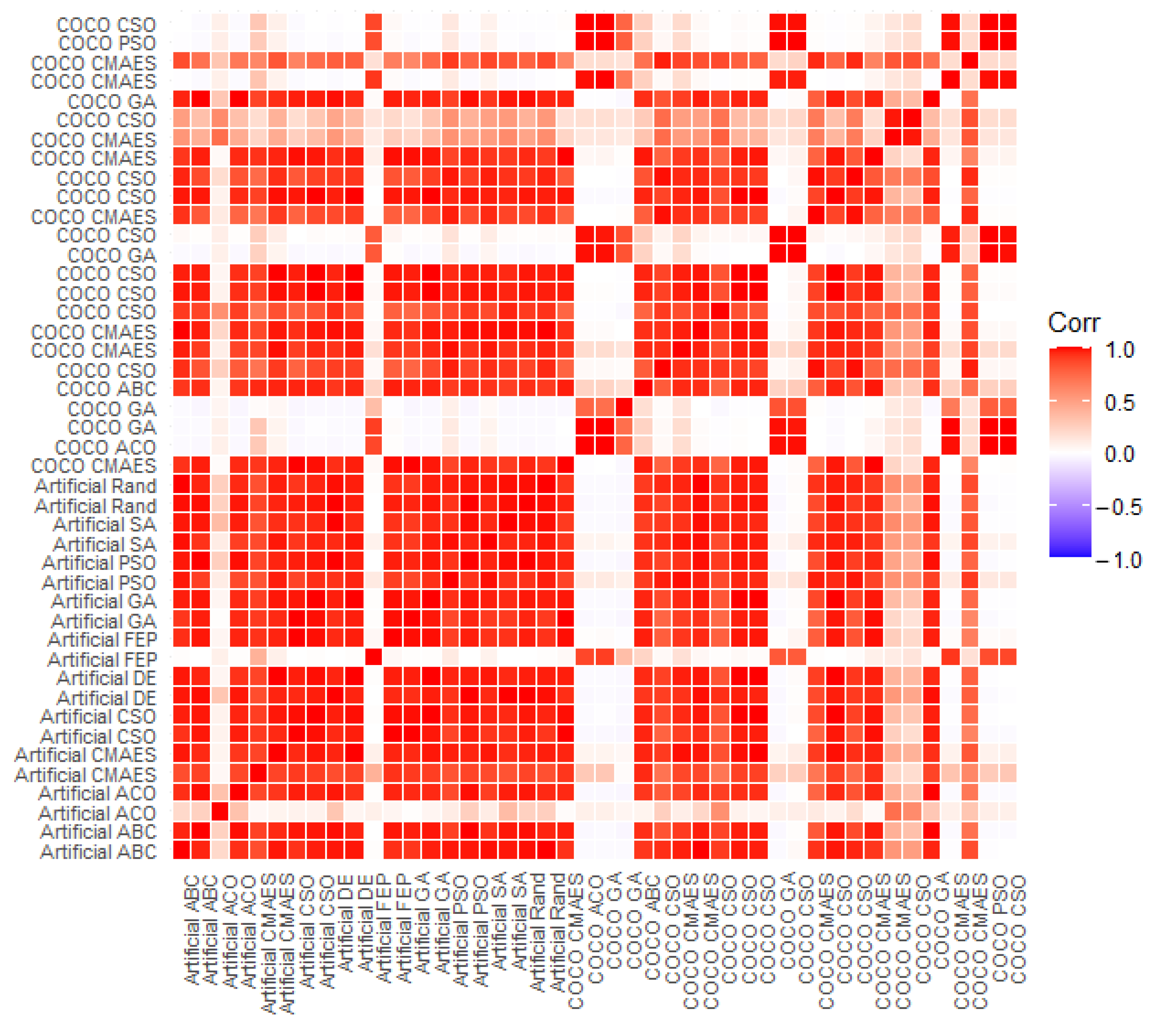
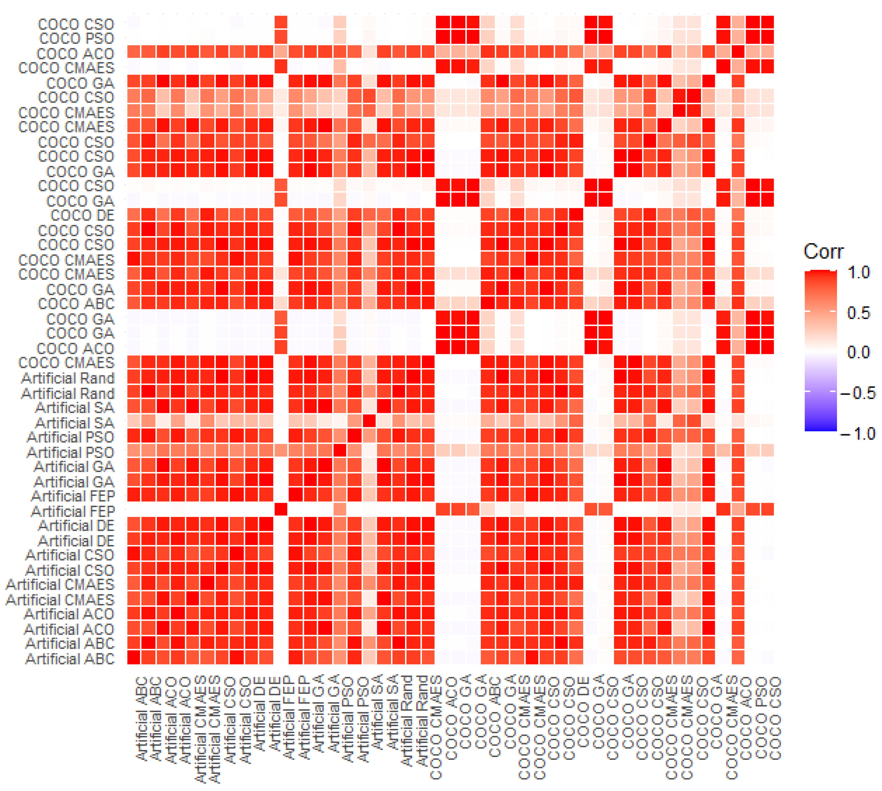
The results of the correlation analysis calculated using Pearson correlation are shown in Figure 2, Figure 3 and Figure 4. The Figures show the correlation between the COCO instances and the artificial instances, using the 44 instance samples that were described earlier in this section.
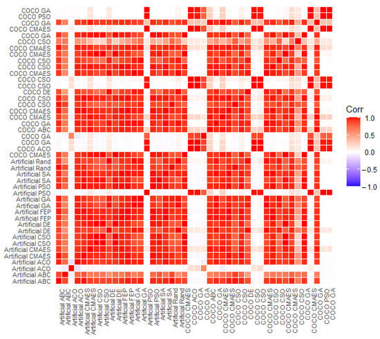
Figure 2.
Correlation between the artificial and the COCO problems, after the COCO problems have been projected to the SVD subspace of the generated problems, using all landscape features. The labels describe the problem set that the features belong to, as well the class of the instance (the algorithm that best solved the instance).
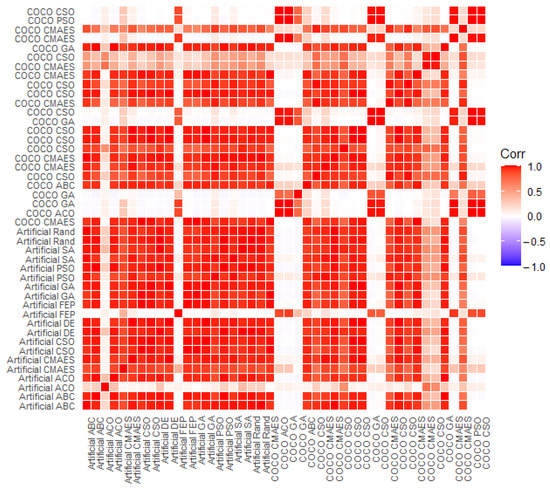
Figure 3.
Correlation between the artificial and the COCO problems, using an alternative sampling.
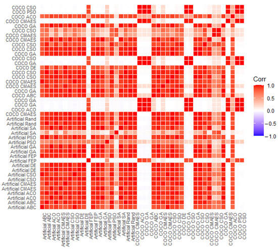
Figure 4.
Correlation between the artificial and the COCO problems, using an alternative sampling.
While the three figures are not exactly the same, we can see that their structure is broadly the same. We can see that there is large correlation between most of the artificial problems, with some exceptions, for example the first ACO and PSO instances in Figure 2. However, the classes these exceptions belong to vary based on the problems that are sampled.
The COCO instances are less sensitive to sampling, as the sampling of the COCO instances is performed based on the base COCO problem. Because of this, all three visualizations produce similar results for the COCO instances. We can see that the COCO instances form two distinct groups where instances are correlated with each other, but not with the instances in the other group.
The correlation between the artificial and the COCO instances produces interesting results. We can see that of the two COCO groups, one is correlated with the majority of the artificial problems, while the second is correlated with the minority of artificial problems. In general, instances with a specific best performing algorithm are not correlated with one another, which explains the poor transfer learning results.
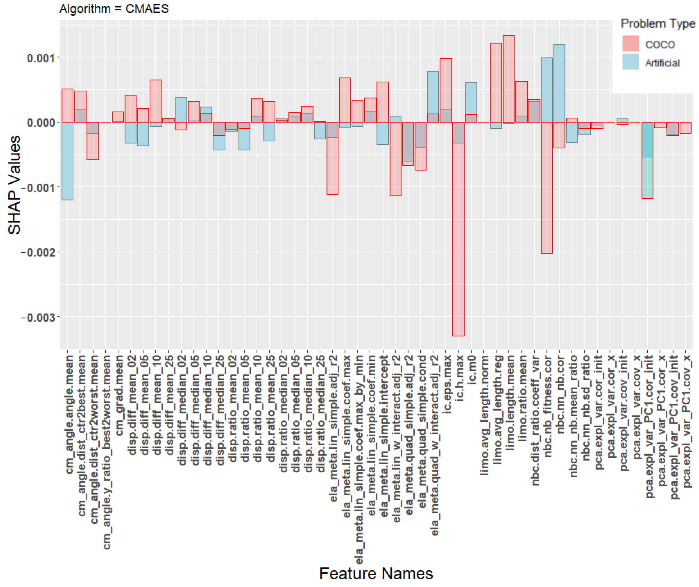
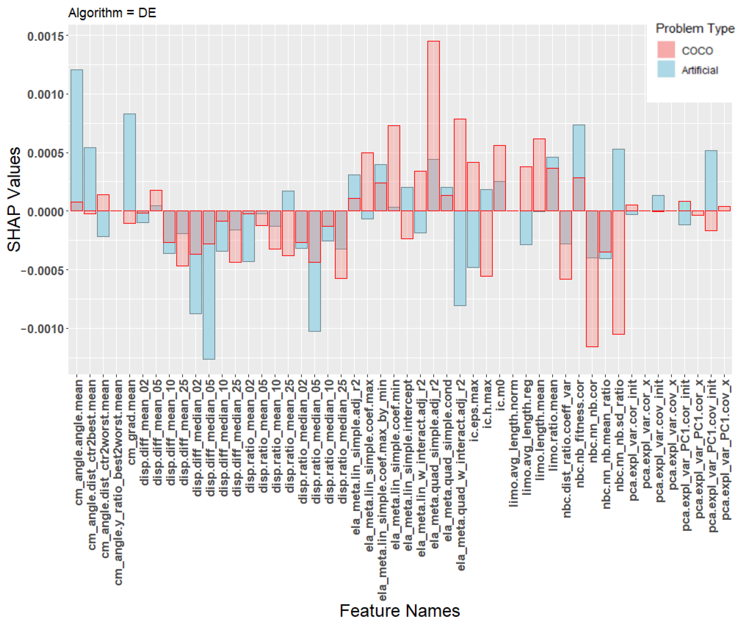
In order to better understand the poor transfer learning performance, Figure 5, Figure 6 and Figure 7 show the SHAP values of the machine learning models. The SHAP values are calculated individually for each training instance and then averaged based on the class the instance belongs to. This gives a total of 10 sets of SHAP values. The landscape features were calculated using the python library shap [39] using default parameters. Each plot contains SHAP values for two machine learning models, one trained on the artificial problems (blue) and one trained on the COCO problems (red). Each figure shows the average contribution of each feature towards one specific algorithm class, specifically CSO, CMA-ES, or the DE classes.
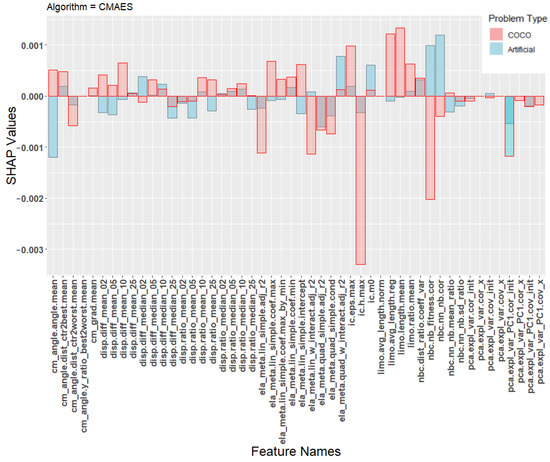
Figure 5.
SHAP values for the prediction model for the algorithm CMAES.
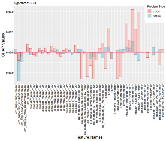
Figure 6.
SHAP values for the prediction model for the algorithm CSO.
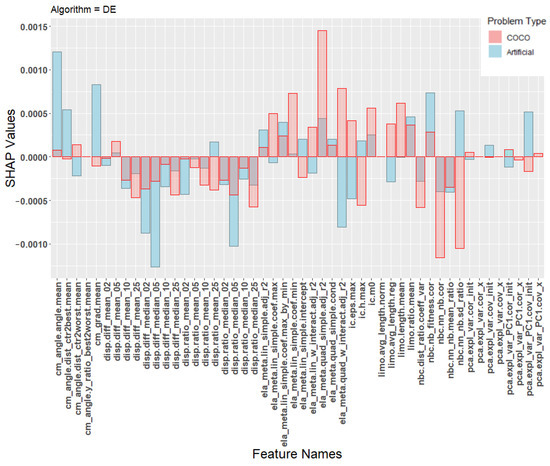
Figure 7.
SHAP values for the prediction model for the algorithm DE.
Due to space constraints, we chose to focus only on these three classes when presenting the results of the SHAP analysis. These classes were chosen because they represent the majority of all classifications of the transfer model, as seen in the confusion matrix in Table 8. Additional plots for the other classes are available at an online repository (https://github.com/UrbanSkv/ela-transfer-learning, (accessed on 30 December 2021)). We can see that all three figures show drastically different levels of feature importance between the artificial and the COCO model. Similar results were observed in all other classes. From this, it is clear that the two models consider different landscape features when making their predictions, which provides a possible explanation for the the poor transfer learning results.
5. Discussion
While the overall results of the transfer learning experiment appear poor, we believe these experiments still raise a number of important points of discussion.
The first point is to highlight the importance of the training and testing set having similar problems in order for machine learning to produce good results. This is easily seen from the two different variations of the models that are both trained and tested on the COCO instances. If the training and testing sets are split per instance, both the training and testing sets contain all 24 base COCO problems, which results in good machine learning performance. However, if the sets are split per problem, than the testing set will always contain only one base COCO problem, which is absent from the training set. This results in poor machine learning performance. Similar results are seen when a model is trained on the artificial instances and tested on the COCO instances.
The correlation analysis has shown that a large number of both the COCO and the artificial problems are highly correlated within their own set of problems. This explains the results of the transfer learning, as a model trained on one set would perform poorly on the other. In addition, this might suggest that only using a single benchmark set, such as the COCO set, might not provide enough algorithm variety to properly assess algorithm performance. The lack of variety in this problem set has already been shown in prior work [18], which also presented a method for expanding the problem set using automatically generated problems. In our work, we have shown the benefit of algorithm generation from a practical perspective, as the combined set of COCO and artificial problems achieved a higher accuracy than the models trained on the artificial set or on the COCO problems when using problem based cross validation.
It is possible that transfer learning could be improved by a better choice of artificial problem generator. While we have attempted to create a balanced set of artificial problems by ensuring a balanced distribution of classes, this only created a balanced distribution according to the performance space of the algorithms, and not the problem space. However, this, as well as the requirement that generated problems should only have a single best performing algorithm, likely introduced an additional bias to our set of problems. Because of this, it is possible a problem generator that could create a set of problems balanced in terms of their landscape features would produce better transfer learning results. It would also be interesting to attempt to perform transfer learning results on real world problems rather than the COCO benchmark problems. Unfortunately, real life problems are hard to acquire in large numbers.
The analysis of the SHAP values has shown that there are large differences in the importance of landscape features between the models trained on the COCO and the artificial problems. However, these differences are not the same for all landscape features, as some landscape features have much larger differences than the others. This could indicate that only some of the landscape features are poorly suited for transfer learning, possibly because they do not generalize well across different problems. We plan to conduct a much more thorough analysis of the SHAP values in order to determine if they can provide useful information in terms of transfer learning performance.
Finally, we note that it is important to take into account inherent differences in problem design between different problem sets. In this paper, we compared two different sets of instances with a large difference in design. The artificial generator removed all instances where there were multiple algorithms with no statistical difference in performance, and contained only a single best performing algorithm, while some COCO instances were solved equally well by a large number of algorithms. This difference in design likely led to the two problem sets containing different instances, which resulted in poor transfer learning results. It is possible that a proper multi-label classification experiment would achieve better results at transfer learning. However, we consider this out of scope for this paper, as it would require a modification of the original artificial problem generation procedure, as well as a machine learning model trained on multi-label artificial data using an appropriate multi-label machine learning algorithm.
6. Conclusions
In this paper, we have examined an attempt at using transfer learning to select the best performing optimization algorithm on the COCO benchmark instances by using an algorithm selection model trained on a separate set of artificially generated problems. This model achieved an accuracy of 0.43, which was similar to the accuracy of the model trained and tested on the artificial problem set (0.50) as well as the model trained and tested on the COCO set using problem based cross validation (0.49). However, a model trained and tested on the COCO problems using instance based cross validation achieved a much higher accuracy of 0.88.
This highlights the importance of the training and testing sets containing similar problems. Only the model trained and tested on the COCO problems using instance based cross validation contained similar problems in both of the training and testing sets, and this model achieved a much higher accuracy than the others.
While this particular transfer learning experiment did not produce great results, there are natural options for further work, particularly in examining transfer learning using different problem sets. We believe that the poor results were caused by the two sets of problems containing very distinct problems. Using a different problem generator could improve results. In addition to examining benchmark problems, it would also be important to analyze transfer learning from a real-world perspective. As there is only a limited number of real-world benchmark problems available, artificial problem generation or surrogate modeling could be useful here. If the artificial problem generator was modified to also produce problems where multiple algorithms are allowed to achieve similar performance to the best performing algorithm, it is possible the generator would create problems that are much more similar to the COCO problem set. In this case, multi-label classification would be a natural avenue for future work, and could improve transfer learning results.
Further research could also focus on improving machine learning results. In this paper, we were focused purely on comparing the results between different training and testing sets, and as such did not devote a large amount of attention to maximizing machine learning performance. Further research could be done on determining the optimal parameters and machine learning algorithms to use for transfer learning, including the use of more advanced machine learning approaches such as neural networks, or by incorporating state-of-the-art transfer learning techniques described in [16] that were already shown to be effective in other domains.
Finally, we plan to conduct a more comprehensive study on the explainability of the transfer learning model using SHAP values. We have seen that the values can be used to show a distinct difference between the models learned on the artificial and the COCO problems. However, in this article we only analyzed the average SHAP values for each algorithm. In the future, we would like to greatly expand our analysis by examining the influence of the ELA features on each individual instance, rather than the average values in order to more thoroughly analyze why the transfer learning performs poorly, and how to improve it.
Author Contributions
Conceptualization, U.Š., T.E. and P.K.; methodology, U.Š., T.E. and P.K.; software, U.Š. and T.E.; validation, U.Š., T.E. and P.K.; formal analysis, U.Š., T.E. and P.K.; investigation, U.Š. and T.E.; writing—original draft preparation, U.Š.; writing—review and editing, U.Š., T.E. and P.K.; visualization, U.Š. and T.E.; supervision, T.E. and P.K.; funding acquisition, U.Š., T.E. and P.K. All authors have read and agreed to the published version of the manuscript.
Funding
This research was funded by the Slovenian Research Agency (research core funding No. P2-0098, project No. Z2-1867, and young researcher funding No. Pr-08987).
Institutional Review Board Statement
Not applicable.
Informed Consent Statement
Not applicable.
Data Availability Statement
The data presented in this study and the software used are openly available in https://github.com/UrbanSkv/ela-transfer-learning, accessed on 30 December 2021.
Conflicts of Interest
The authors declare no conflict of interest. The funders had no role in the design of the study; in the collection, analyses, or interpretation of data; in the writing of the manuscript, or in the decision to publish the results.
Abbreviations
The following abbreviations are used in this manuscript:
| COCO | Comparing Continuous Optimizers |
| ELA | Exploratory Landscape Analysis |
| SHAP | Shapley Additive Explanations |
| ICOP | Interpolated Continuous Optimisation Problems |
| ABC | Artificial Bee Colony |
| ACO | Ant Colony Optimization |
| CSO | Competitive Swarm Optimizer |
| DE | Differential Evolution |
| FEP | Fast Evolutionary Programming |
| GA | Genetic Algorithm |
| PSO | Particle Swarm Optimization |
| SA | Simulated Annealing |
| Rand | Random Search |
| CMA-ES | Covariance matrix adaptation |
| SVD | Singular Value Decomposition |
References
- Rice, J.R. The algorithm selection problem. In Advances in Computers; Elsevier: Amsterdam, The Netherlands, 1976; Volume 15, pp. 65–118. [Google Scholar]
- Wolpert, D.H.; Macready, W.G. No free lunch theorems for optimization. IEEE Trans. Evol. Comput. 1997, 1, 67–82. [Google Scholar] [CrossRef] [Green Version]
- Tian, Y.; Peng, S.; Zhang, X.; Rodemann, T.; Tan, K.C.; Jin, Y. A Recommender System for Metaheuristic Algorithms for Continuous Optimization Based on Deep Recurrent Neural Networks. IEEE Trans. Artif. Intell. 2020, 1, 5–18. [Google Scholar] [CrossRef]
- Hansen, N.; Auger, A.; Ros, R.; Mersmann, O.; Tušar, T.; Brockhoff, D. COCO: A platform for comparing continuous optimizers in a black-box setting. Optim. Methods Softw. 2021, 36, 114–144. [Google Scholar] [CrossRef]
- Mersmann, O.; Preuss, M.; Trautmann, H. Benchmarking Evolutionary Algorithms: Towards Exploratory Landscape Analysis. In Parallel Problem Solving from Nature, PPSN XI; Schaefer, R., Cotta, C., Kołodziej, J., Rudolph, G., Eds.; Springer: Berlin/Heidelberg, Germany, 2010; pp. 73–82. [Google Scholar]
- Mersmann, O.; Bischl, B.; Trautmann, H.; Preuss, M.; Weihs, C.; Rudolph, G. Exploratory landscape analysis. In Proceedings of the 2011 Annual Conference on Genetic and Evolutionary Computation, Dublin, Ireland, 12–16 July 2011; pp. 829–836. [Google Scholar]
- Kerschke, P.; Trautmann, H. Automated algorithm selection on continuous black-box problems by combining exploratory landscape analysis and machine learning. Evol. Comput. 2019, 27, 99–127. [Google Scholar] [CrossRef] [Green Version]
- Lundberg, S.M.; Lee, S.I. A unified approach to interpreting model predictions. In Proceedings of the 31st International Conference on Neural Information Processing Systems, Long Beach, CA, USA, 4–9 December 2017; pp. 4768–4777. [Google Scholar]
- Kerschke, P.; Hoos, H.H.; Neumann, F.; Trautmann, H. Automated algorithm selection: Survey and perspectives. Evol. Comput. 2019, 27, 3–45. [Google Scholar] [CrossRef] [PubMed]
- Jankovic, A.; Eftimov, T.; Doerr, C. Towards Feature-Based Performance Regression Using Trajectory Data. In Applications of Evolutionary Computation (EvoApplications 2021); Springer: Berlin/Heidelberg, Germany, 2021; Volume 12694, pp. 601–617. [Google Scholar]
- Belkhir, N.; Dreo, J.; Savéant, P.; Schoenauer, M. Per instance algorithm configuration of CMA-ES with limited budget. In Proceedings of the Genetic and Evolutionary Computation Conference (GECCO’17), Berlin, Germany, 15–19 July 2017; pp. 681–688. [Google Scholar] [CrossRef] [Green Version]
- Muñoz, M.A.; Sun, Y.; Kirley, M.; Halgamuge, S.K. Algorithm selection for black-box continuous optimization problems: A survey on methods and challenges. Inf. Sci. 2015, 317, 224–245. [Google Scholar] [CrossRef] [Green Version]
- Derbel, B.; Liefooghe, A.; Vérel, S.; Aguirre, H.E.; Tanaka, K. New features for continuous exploratory landscape analysis based on the SOO tree. In Proceedings of the Foundations of Genetic Algorithms (FOGA’19), Potsdam, Germany, 27–29 August 2019; pp. 72–86. [Google Scholar] [CrossRef]
- Jankovic, A.; Doerr, C. Landscape-aware fixed-budget performance regression and algorithm selection for modular CMA-ES variants. In Proceedings of the 2020 Genetic and Evolutionary Computation Conference, Cancún, Mexico, 8–12 July 2020; pp. 841–849. [Google Scholar]
- Jankovic, A.; Popovski, G.; Eftimov, T.; Doerr, C. The Impact of Hyper-Parameter Tuning for Landscape-Aware Performance Regression and Algorithm Selection. arXiv 2021, arXiv:2104.09272. [Google Scholar]
- Zhuang, F.; Qi, Z.; Duan, K.; Xi, D.; Zhu, Y.; Zhu, H.; Xiong, H.; He, Q. A comprehensive survey on transfer learning. Proc. IEEE 2020, 109, 43–76. [Google Scholar] [CrossRef]
- Lacroix, B.; McCall, J. Limitations of benchmark sets and landscape features for algorithm selection and performance prediction. In Proceedings of the Genetic and Evolutionary Computation Conference Companion, Prague, Czech Republic, 13–17 July 2019; pp. 261–262. [Google Scholar]
- Muñoz, M.A.; Smith-Miles, K. Generating new space-filling test instances for continuous black-box optimization. Evol. Comput. 2020, 28, 379–404. [Google Scholar] [CrossRef]
- Lacroix, B.; Christie, L.A.; McCall, J.A. Interpolated continuous optimisation problems with tunable landscape features. In Proceedings of the Genetic and Evolutionary Computation Conference Companion, Berlin, Germany, 15–19 July 2017; pp. 169–170. [Google Scholar]
- Fischbach, A.; Bartz-Beielstein, T. Improving the reliability of test functions generators. Appl. Soft Comput. 2020, 92, 106315. [Google Scholar] [CrossRef]
- Eftimov, T.; Popovski, G.; Renau, Q.; Korošec, P.; Doerr, C. Linear Matrix Factorization Embeddings for Single-objective Optimization Landscapes. In Proceedings of the 2020 IEEE Symposium Series on Computational Intelligence (SSCI), Canberra, ACT, Australia, 1–4 December 2020; pp. 775–782. [Google Scholar] [CrossRef]
- Škvorc, U.; Eftimov, T.; Korošec, P. Understanding the problem space in single-objective numerical optimization using exploratory landscape analysis. Appl. Soft Comput. 2020, 90, 106138. [Google Scholar] [CrossRef]
- Karaboga, D. An Idea Based on Honey Bee Swarm for Numerical Optimization; Technical Report; Citeseer: Kayseri, Turkey, 2005. [Google Scholar]
- Socha, K.; Dorigo, M. Ant colony optimization for continuous domains. Eur. J. Oper. Res. 2008, 185, 1155–1173. [Google Scholar] [CrossRef] [Green Version]
- Cheng, R.; Jin, Y. A competitive swarm optimizer for large scale optimization. IEEE Trans. Cybern. 2014, 45, 191–204. [Google Scholar] [CrossRef] [PubMed]
- Storn, R.; Price, K. Differential evolution—A simple and efficient heuristic for global optimization over continuous spaces. J. Glob. Optim. 1997, 11, 341–359. [Google Scholar] [CrossRef]
- Yao, X.; Liu, Y.; Lin, G. Evolutionary programming made faster. IEEE Trans. Evol. Comput. 1999, 3, 82–102. [Google Scholar]
- Deb, K.; Agrawal, R.B. Simulated binary crossover for continuous search space. Complex Syst. 1995, 9, 115–148. [Google Scholar]
- Deb, K.; Goyal, M. A combined genetic adaptive search (GeneAS) for engineering design. Comput. Sci. Inform. 1996, 26, 30–45. [Google Scholar]
- Eberhart, R.; Kennedy, J. A new optimizer using particle swarm theory. MHS’95. In Proceedings of the Sixth International Symposium on Micro Machine and Human Science, Nagoya, Japan, 4–6 October 1995; pp. 39–43. [Google Scholar]
- Van Laarhoven, P.J.; Aarts, E.H. Simulated annealing. In Simulated Annealing: Theory and Applications; Springer: Berlin/Heidelberg, Germany, 1987; pp. 7–15. [Google Scholar]
- Zabinsky, Z.B. Random search algorithms. In Wiley Encyclopedia of Operations Research and Management Science; Wiley: Hoboken, NJ, USA, 2010. [Google Scholar]
- Hansen, N.; Ostermeier, A. Completely derandomized self-adaptation in evolution strategies. Evol. Comput. 2001, 9, 159–195. [Google Scholar] [CrossRef]
- Breiman, L. Random forests. Mach. Learn. 2001, 45, 5–32. [Google Scholar] [CrossRef] [Green Version]
- Kerschke, P.; Trautmann, H. Comprehensive Feature-Based Landscape Analysis of Continuous and Constrained Optimization Problems Using the R-Package Flaccos. In Applications in Statistical Computing: From Music Data Analysis to Industrial Quality Improvement; Bauer, N., Ickstadt, K., Lübke, K., Szepannek, G., Trautmann, H., Vichi, M., Eds.; Springer International Publishing: Cham, Germany, 2019; pp. 93–123. [Google Scholar]
- Ying, X. An overview of overfitting and its solutions. J. Phys. Conf. Ser. 2019, 1168, 022022. [Google Scholar] [CrossRef]
- Liaw, A.; Wiener, M. Classification and Regression by randomForest. R News 2002, 2, 18–22. [Google Scholar]
- Friedman, J.; Hastie, T.; Tibshirani, R.; Hastie, T. The Elements of Statistical Learning; Springer Series in Statistics New York; Springer: Berlin/Heidelberg, Germany, 2001; Volume 1. [Google Scholar]
- Lundberg, S.M. Shap. Available online: https://github.com/slundberg/shap (accessed on 30 December 2021).
Publisher’s Note: MDPI stays neutral with regard to jurisdictional claims in published maps and institutional affiliations. |
© 2022 by the authors. Licensee MDPI, Basel, Switzerland. This article is an open access article distributed under the terms and conditions of the Creative Commons Attribution (CC BY) license (https://creativecommons.org/licenses/by/4.0/).

