
Semi-Local Integration Measure of Node Importance


Abstract
:1. Introduction
Related Work
2. Semi-Local Intregation Centrality
2.1. Definition
- —denotes the of the node ;
- —denotes the () of the node ;
- —denotes the edge between the nodes ;
- —denotes the weight of the edge ;
- —denotes the set of edges incident to , ;
- —denotes the cycle basis of the graph G;
- —denotes the number of cycles in that contain the edge .
2.2. Discussion on Definition
2.3. in Unweighted Graphs
3. Application of in Lexical Networks
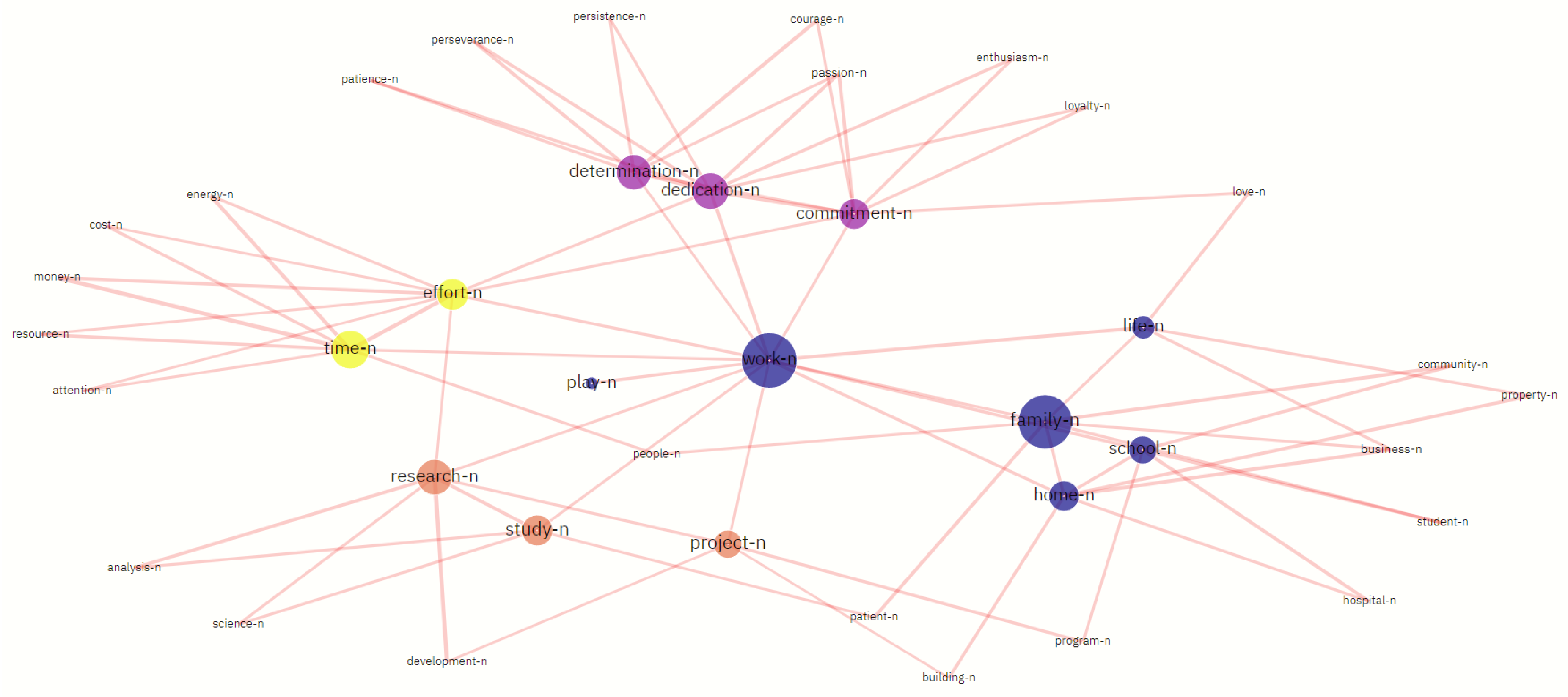
3.1. Application of in the Analysis of Sense Structure
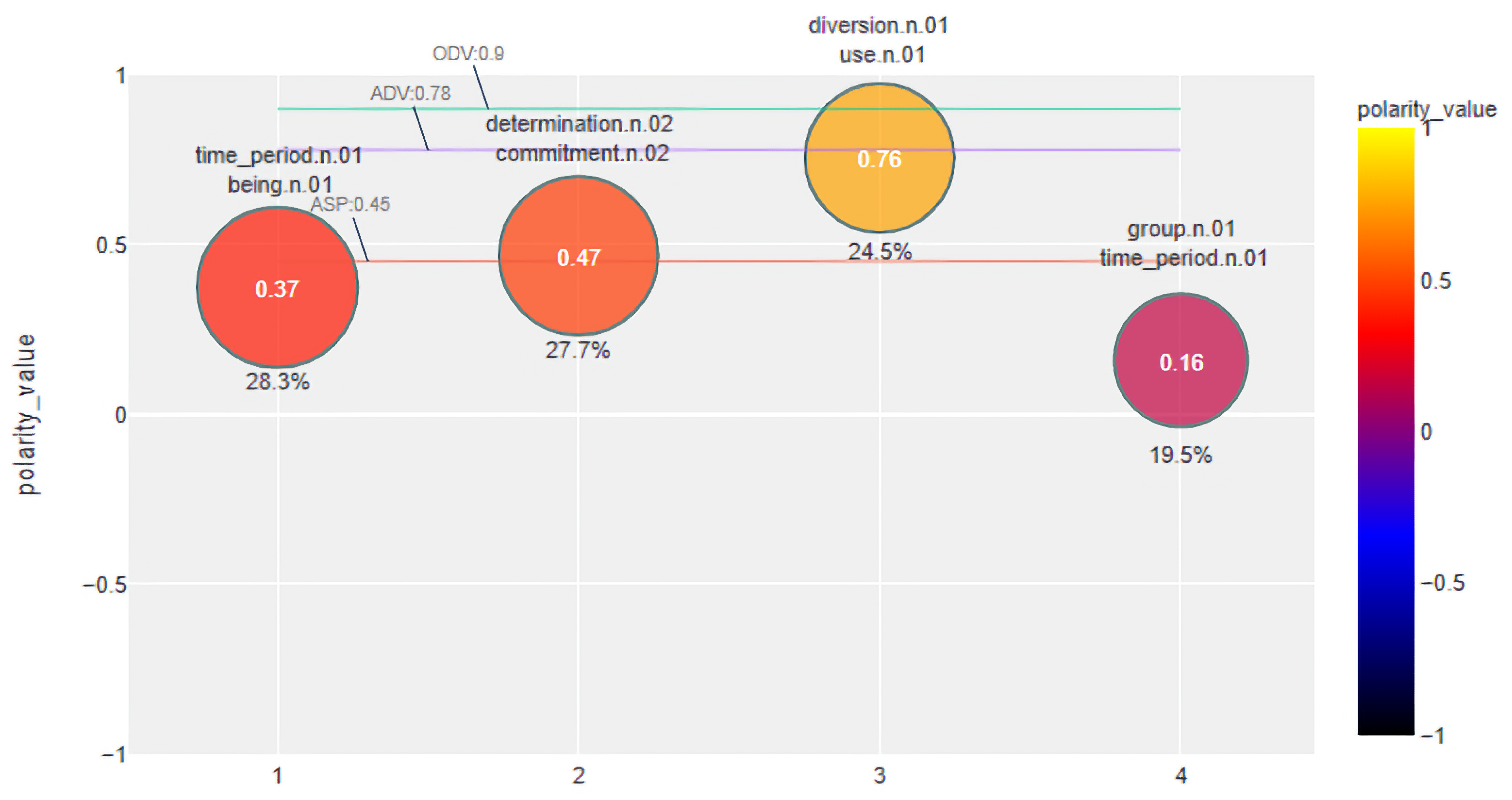
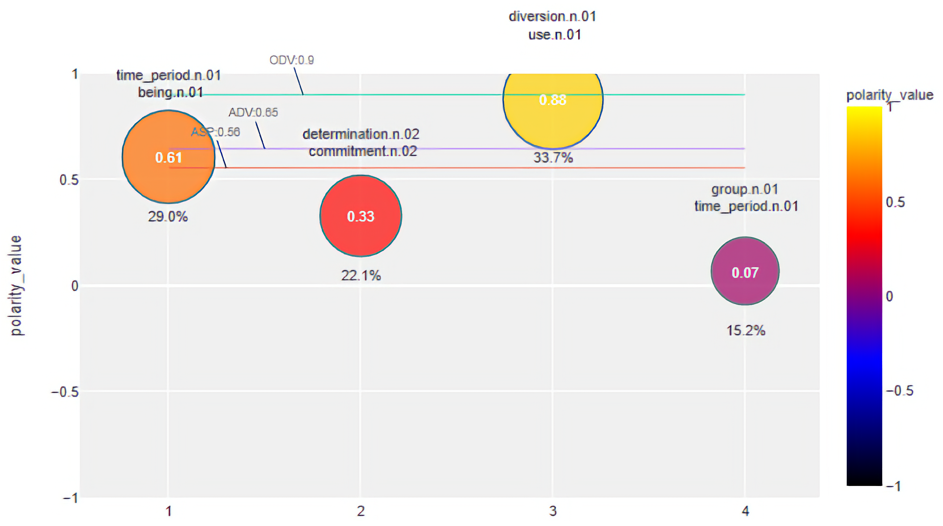
3.2. Application of in Sentiment Analysis
3.3. Further Areas of Applications
4. Conclusions
Supplementary Materials
Author Contributions
Funding
Institutional Review Board Statement
Informed Consent Statement
Data Availability Statement
Conflicts of Interest
References
- Freeman, L.C. Centrality in social networks conceptual clarification. Soc. Netw. 1978, 1, 215–239. [Google Scholar] [CrossRef] [Green Version]
- Newman, M. Networks; Oxford University Press: Oxford, UK, 2018. [Google Scholar]
- Das, K.; Samanta, S.; Pal, M. Study on centrality measures in social networks: A survey. Soc. Netw. Anal. Min. 2018, 8, 13. [Google Scholar] [CrossRef]
- Gleich, D.F. PageRank beyond the Web. SIAM Rev. 2015, 57, 321–363. [Google Scholar] [CrossRef]
- Li, G.; Li, M.; Wang, J.; Li, Y.; Pan, Y. United neighborhood closeness centrality and orthology for predicting essential proteins. IEEE/ACM Trans. Comput. Biol. Bioinform. 2018, 17, 1451–1458. [Google Scholar] [CrossRef]
- Riondato, M.; Upfal, E. Abra: Approximating betweenness centrality in static and dynamic graphs with rademacher averages. ACM Trans. Knowl. Discov. Data (TKDD) 2018, 12, 1–38. [Google Scholar] [CrossRef]
- Brin, S.; Page, L. The anatomy of a large-scale hypertextual web search engine. Comput. Netw. ISDN Syst. 1998, 30, 107–117. [Google Scholar] [CrossRef]
- Dong, J.; Ye, F.; Chen, W.; Wu, J. Identifying influential nodes in complex networks via semi-local centrality. In Proceedings of the 2018 IEEE International Symposium on Circuits and Systems (ISCAS), Florence, Italy, 27–30 May 2018; pp. 1–5. [Google Scholar]
- Liu, J.; Xiong, Q.; Shi, W.; Shi, X.; Wang, K. Evaluating the importance of nodes in complex networks. Phys. A Stat. Mech. Its Appl. 2016, 452, 209–219. [Google Scholar] [CrossRef] [Green Version]
- Wang, J.; Rong, L.; Guo, T. A new measure method of network node importance based on local characteristics. J. Dalian Univ. Technol. 2010, 50, 822–826. [Google Scholar]
- Ren, Z.M.; Shao, F.; Liu, J.G.; Guo, Q.; Wang, B.H. Node importance measurement based on the degree and clustering coefficient information. Acta Phys. Sin. 2013, 62, 128901. [Google Scholar]
- Chen, D.; Lü, L.; Shang, M.S.; Zhang, Y.C.; Zhou, T. Identifying influential nodes in complex networks. Phys. A Stat. Mech. Its Appl. 2012, 391, 1777–1787. [Google Scholar] [CrossRef] [Green Version]
- ConGraCNet Application. Available online: https://github.com/bperak/ConGraCNet (accessed on 23 January 2022).
- Semi-Local Integration Measure. Available online: https://github.com/sbujacic/SLI-Node-Importance-Measure (accessed on 23 January 2022).
- Guze, S. Graph theory approach to the vulnerability of transportation networks. Algorithms 2019, 12, 270. [Google Scholar] [CrossRef] [Green Version]
- Canright, G.; Engø-Monsen, K. Roles in networks. Sci. Comput. Program. 2004, 53, 195–214. [Google Scholar] [CrossRef] [Green Version]
- Lawyer, G. Understanding the influence of all nodes in a network. Sci. Rep. 2015, 5, 8665. [Google Scholar] [CrossRef] [PubMed] [Green Version]
- Jones, P.J.; Ma, R.; McNally, R.J. Bridge centrality: A network approach to understanding comorbidity. Multivar. Behav. Res. 2021, 56, 353–367. [Google Scholar] [CrossRef] [PubMed]
- Kitsak, M.; Gallos, L.; Havlin, S.; Liljeros, F.; Muchnik, L.; Eugene Stanley, H.; Makse, H. Identification of influential spreaders in complex networks. Nat. Phys. 2010, 6, 888–893. [Google Scholar] [CrossRef] [Green Version]
- Meghanathan, N. Neighborhood-based bridge node centrality tuple for complex network analysis. Appl. Netw. Sci. 2021, 47, 888–893. [Google Scholar] [CrossRef]
- Newman, M.E. Analysis of weighted networks. Phys. Rev. E 2004, 70, 056131. [Google Scholar] [CrossRef] [Green Version]
- Opsahl, T.; Colizza, V.; Panzarasa, P.; Ramasco, J.J. Prominence and control: The weighted rich-club effect. Phys. Rev. Lett. 2008, 101, 168702. [Google Scholar] [CrossRef] [Green Version]
- Segarra, S.; Ribeiro, A. Stability and continuity of centrality measures in weighted graphs. IEEE Trans. Signal Process. 2015, 64, 543–555. [Google Scholar] [CrossRef] [Green Version]
- Opsahl, T.; Agneessens, F.; Skvoretz, J. Node centrality in weighted networks: Generalizing degree and shortest paths. Soc. Netw. 2010, 32, 245–251. [Google Scholar] [CrossRef]
- Nastase, V.; Mihalcea, R.; Radev, D.R. A survey of graphs in natural language processing. Nat. Lang. Eng. 2015, 21, 665–698. [Google Scholar] [CrossRef] [Green Version]
- Perak, B.; Ban Kirigin, T. Corpus-Based Syntactic-Semantic Graph Analysis: Semantic Domains of the Concept Feeling. Raspr. Časopis Instituta Za Hrvat. Jez. I Jezikoslovlje 2020, 46, 493–532. [Google Scholar] [CrossRef]
- Ban Kirigin, T.; Bujačić Babić, S.; Perak, B. Lexical Sense Labeling and Sentiment Potential Analysis Using Corpus-Based Dependency Graph. Mathematics 2021, 9, 1449. [Google Scholar] [CrossRef]
- Perak, B.; Ban Kirigin, T. Dependency-based Labeling of Associative Lexical Communities. In Proceedings of the Central European Conference on Information and Intelligent Systems (CECIIS 2021), Varaždin, Croatia, 13–15 October 2021; pp. 34–42. [Google Scholar]
- Van Oirsouw, R.R. The Syntax of Coordination; Routledge: New York, NY, USA, 2019. [Google Scholar]
- Langacker, R.W. Investigations in Cognitive Grammar; De Gruyter Mouton, 2009; Available online: https://doi.org/10.1515/9783110214369 (accessed on 23 January 2022).
- Stefanowitsch, A.; Gries, S.T. Collostructions: Investigating the interaction of words and constructions. Int. J. Corpus Linguist. 2003, 8, 209–243. [Google Scholar] [CrossRef] [Green Version]
- Raghavan, U.N.; Albert, R.; Kumara, S. Near linear time algorithm to detect community structures in large-scale networks. Phys. Rev. E 2007, 76, 036106. [Google Scholar] [CrossRef] [PubMed] [Green Version]
- Latapy, M. Main-memory triangle computations for very large (sparse (power-law)) graphs. Theor. Comput. Sci. 2008, 407, 458–473. [Google Scholar] [CrossRef]
- Blondel, V.D.; Guillaume, J.L.; Lambiotte, R.; Lefebvre, E. Fast unfolding of communities in large networks. J. Stat. Mech. Theory Exp. 2008, 2008, P10008. [Google Scholar] [CrossRef] [Green Version]
- Traag, V.A.; Waltman, L.; Van Eck, N.J. From Louvain to Leiden: Guaranteeing well-connected communities. Sci. Rep. 2019, 9, 5233. [Google Scholar] [CrossRef]
- Cambria, E.; Li, Y.; Xing, F.Z.; Poria, S.; Kwok, K. SenticNet 6: Ensemble application of symbolic and subsymbolic AI for sentiment analysis. In Proceedings of the 29th ACM International Conference on Information & Knowledge Management, Online, 19–23 October 2020; pp. 105–114. Available online: https://doi.org/10.1145/3340531.3412003 (accessed on 23 January 2022).
- Sentic. Available online: https://sentic.net/ (accessed on 23 January 2022).
- Gatti, L.; Guerini, M.; Turchi, M. SentiWords: Deriving a high precision and high coverage lexicon for sentiment analysis. IEEE Trans. Affect. Comput. 2015, 7, 409–421. [Google Scholar] [CrossRef] [Green Version]
- Gao, W.; Wu, H.; Siddiqui, M.K.; Baig, A.Q. Study of biological networks using graph theory. Saudi J. Biol. Sci. 2018, 25, 1212–1219. [Google Scholar] [CrossRef]
- Venkatraman, Y.; Balas, V.E.; Rad, D.; Narayanaa, Y.K. Graph Theory Applications to Comprehend Epidemics Spread of a Disease. BRAIN. Broad Res. Artif. Intell. Neurosci. 2021, 12, 161–177. [Google Scholar]
- Chakraborty, A.; Dutta, T.; Mondal, S.; Nath, A. Application of graph theory in social media. Int. J. Comput. Sci. Eng. 2018, 6, 722–729. [Google Scholar] [CrossRef]
- Lehmann, S.; Ahn, Y.Y. Complex Spreading Phenomena in Social Systems; Springer: Cham, Switzerland, 2018. [Google Scholar]
- Pătruţ, B.; Popa, I.L. Graph Theory Algorithms for Analysing Political Blogs. In Social Media in Politics; Springer: Cham, Switzerland, 2014; pp. 49–62. [Google Scholar]


| Node | |||||
|---|---|---|---|---|---|
| 40.225 | 6 | 12.65 | 0.594 | 0.148 | |
| 16.225 | 7 | 9.4 | 0.345 | 0.118 | |
| 13.269 | 6 | 7.45 | 0.246 | 0.096 | |
| 9.614 | 5 | 6.1 | 0.147 | 0.076 | |
| 6.961 | 5 | 5.7 | 0.193 | 0.077 | |
| 6.664 | 6 | 5.65 | 0.259 | 0.081 | |
| 1.671 | 2 | 2.7 | 0.024 | 0.035 | |
| 1.238 | 4 | 3.6 | 0.239 | 0.071 | |
| 0.969 | 2 | 2 | 0.0 | 0.029 | |
| 0.569 | 1 | 2 | 0.0 | 0.027 | |
| 0.546 | 2 | 1.4 | 0.0 | 0.022 | |
| 0.39 | 1 | 2 | 0.0 | 0.039 | |
| 0.224 | 1 | 1 | 0.0 | 0.017 | |
| 0.21 | 1 | 1 | 0.0 | 0.018 | |
| 0.166 | 1 | 0.8 | 0.0 | 0.015 | |
| 0.16 | 1 | 0.8 | 0.0 | 0.015 | |
| 0.15 | 1 | 0.75 | 0.0 | 0.014 | |
| 0.149 | 1 | 0.8 | 0.0 | 0.019 | |
| 0.139 | 1 | 0.7 | 0.0 | 0.013 | |
| 0.11 | 1 | 0.6 | 0.0 | 0.013 | |
| 0.088 | 1 | 0.5 | 0.0 | 0.011 | |
| 0.067 | 1 | 0.4 | 0.0 | 0.010 | |
| 0.067 | 1 | 0.4 | 0.0 | 0.011 | |
| 0.067 | 1 | 0.4 | 0.0 | 0.011 | |
| 0.065 | 1 | 0.4 | 0.0 | 0.013 |
| Node | ||||
|---|---|---|---|---|
| 18.433 | 6 | 0.594 | 0.087 | |
| 16.708 | 7 | 0.345 | 0.111 | |
| 15.543 | 6 | 0.246 | 0.091 | |
| 11.437 | 5 | 0.147 | 0.074 | |
| 12.892 | 6 | 0.259 | 0.094 | |
| 9.51 | 5 | 0.193 | 0.077 | |
| 3.512 | 4 | 0.239 | 0.073 | |
| 1.943 | 2 | 0.024 | 0.032 | |
| 1.951 | 2 | 0.0 | 0.032 | |
| 1.882 | 2 | 0.0 | 0.032 | |
| 0.427 | 1 | 0.0 | 0.02 | |
| 0.427 | 1 | 0.0 | 0.02 | |
| 0.418 | 1 | 0.0 | 0.019 | |
| 0.427 | 1 | 0.0 | 0.02 | |
| 0.418 | 1 | 0.0 | 0.019 | |
| 0.407 | 1 | 0.0 | 0.019 | |
| 0.427 | 1 | 0.0 | 0.02 | |
| 0.39 | 1 | 0.0 | 0.022 | |
| 0.418 | 1 | 0.0 | 0.019 | |
| 0.407 | 1 | 0.0 | 0.019 | |
| 0.39 | 1 | 0.0 | 0.022 | |
| 0.418 | 1 | 0.0 | 0.019 | |
| 0.418 | 1 | 0.0 | 0.019 | |
| 0.407 | 1 | 0.0 | 0.019 | |
| 0.39 | 1 | 0.0 | 0.022 |
| Lexeme | SenticNet6 | |||
|---|---|---|---|---|
| work | 96.35 | 6219.4667 | 11.0602 | 0.9 |
| family | 143.21 | 1615.5262 | 10.7711 | 0.883 |
| time | 115.68 | 1057.2845 | 7.7119 | - |
| dedication | 103.43 | 788.0095 | 7.3328 | 0.034 |
| research | 117.88 | 1459.5190 | 7.0717 | 0.883 |
| determination | 108.08 | 1037.9310 | 7.0436 | 0.231 |
| effort | 93.85 | 982.9595 | 6.3767 | 0.037 |
| study | 120.33 | 1687.6012 | 6.2252 | - |
| commitment | 97.82 | 855.6643 | 6.1272 | 0.704 |
| home | 107.3 | 1059.3940 | 6.0986 | - |
| project | 115.6 | 1705.4262 | 5.6272 | 0.9 |
| school | 107.21 | 1129.0250 | 5.6033 | - |
| life | 101.38 | 1188.8881 | 4.6721 | - |
| play | 96.1 | 1677 | 2.5525 | - |
| passion | 24.54 | 0 | 0.3868 | 1 |
| business | 23.7 | 21.0357 | 0.3673 | - |
| money | 18.79 | 0 | 0.1937 | 0.065 |
| SenticNet 6 | Work-n | ||
|---|---|---|---|
| Community | Lexemes | ||
| 1 | life-n, school-n, home-n, family-n, love-n, property-n, business-n, hospital-n, student-n, community-n, program-n, building-n | 0.37 | 0.61 |
| 2 | dedication-n, commitment-n, determination-n, passion-n, perseverance-n, enthusiasm-n, patience-n, loyalty-n, persistence-n, courage-n | 0.47 | 0.33 |
| 3 | work-n, play-n, research-n, study-n, project-n, patient-n, development-n, analysis-n, science-n | 0.76 | 0.88 |
| 4 | effort-n, time-n, money-n, energy-n, resource-n, cost-n, attention-n, people-n | 0.16 | 0.07 |
| : 0.9 | : 0.78 : 0.65 | ||
| : 0.45 : 0.56 |
Publisher’s Note: MDPI stays neutral with regard to jurisdictional claims in published maps and institutional affiliations. |
© 2022 by the authors. Licensee MDPI, Basel, Switzerland. This article is an open access article distributed under the terms and conditions of the Creative Commons Attribution (CC BY) license (https://creativecommons.org/licenses/by/4.0/).
Share and Cite
Ban Kirigin, T.; Bujačić Babić, S.; Perak, B. Semi-Local Integration Measure of Node Importance. Mathematics 2022, 10, 405. https://doi.org/10.3390/math10030405
Ban Kirigin T, Bujačić Babić S, Perak B. Semi-Local Integration Measure of Node Importance. Mathematics. 2022; 10(3):405. https://doi.org/10.3390/math10030405
Chicago/Turabian StyleBan Kirigin, Tajana, Sanda Bujačić Babić, and Benedikt Perak. 2022. "Semi-Local Integration Measure of Node Importance" Mathematics 10, no. 3: 405. https://doi.org/10.3390/math10030405
APA StyleBan Kirigin, T., Bujačić Babić, S., & Perak, B. (2022). Semi-Local Integration Measure of Node Importance. Mathematics, 10(3), 405. https://doi.org/10.3390/math10030405