
Parameters Optimization of Taguchi Method Integrated Hybrid Harmony Search Algorithm for Engineering Design Problems


Abstract
:1. Introduction
- The effect of variable run values on finding the optimum solution by employing different complex benchmark engineering design optimization problems and a real-size engineering design problem, frequently considered in optimization analyzes in the literature has been investigated;
- Taguchi method integrated hybrid harmony search algorithm (TIHHSA) has been generated based on the HSA and Taguchi method, namely the proposed hybridization can be defined as initial optimization for optimum algorithm parameter values of HSA;
- The effect of HSA parameters on the objective function and the optimum number of runs and maximum iterations with optimum HSA control parameters have been examined for different engineering optimization design problems utilizing TIHHSA;
- Whether the variation of the optimum values of the HSA parameters depending on the nature of the engineering design optimization problem has been evaluated;
- According to accomplished optimum results for engineering design optimization problems, the robustness, and the benefits of TIHHSA presented a new method have been interpreted and evaluated with previously reported studies in the literature.
2. Materials and Methods
2.1. Complex Benchmark Engineering Design Optimization Problems
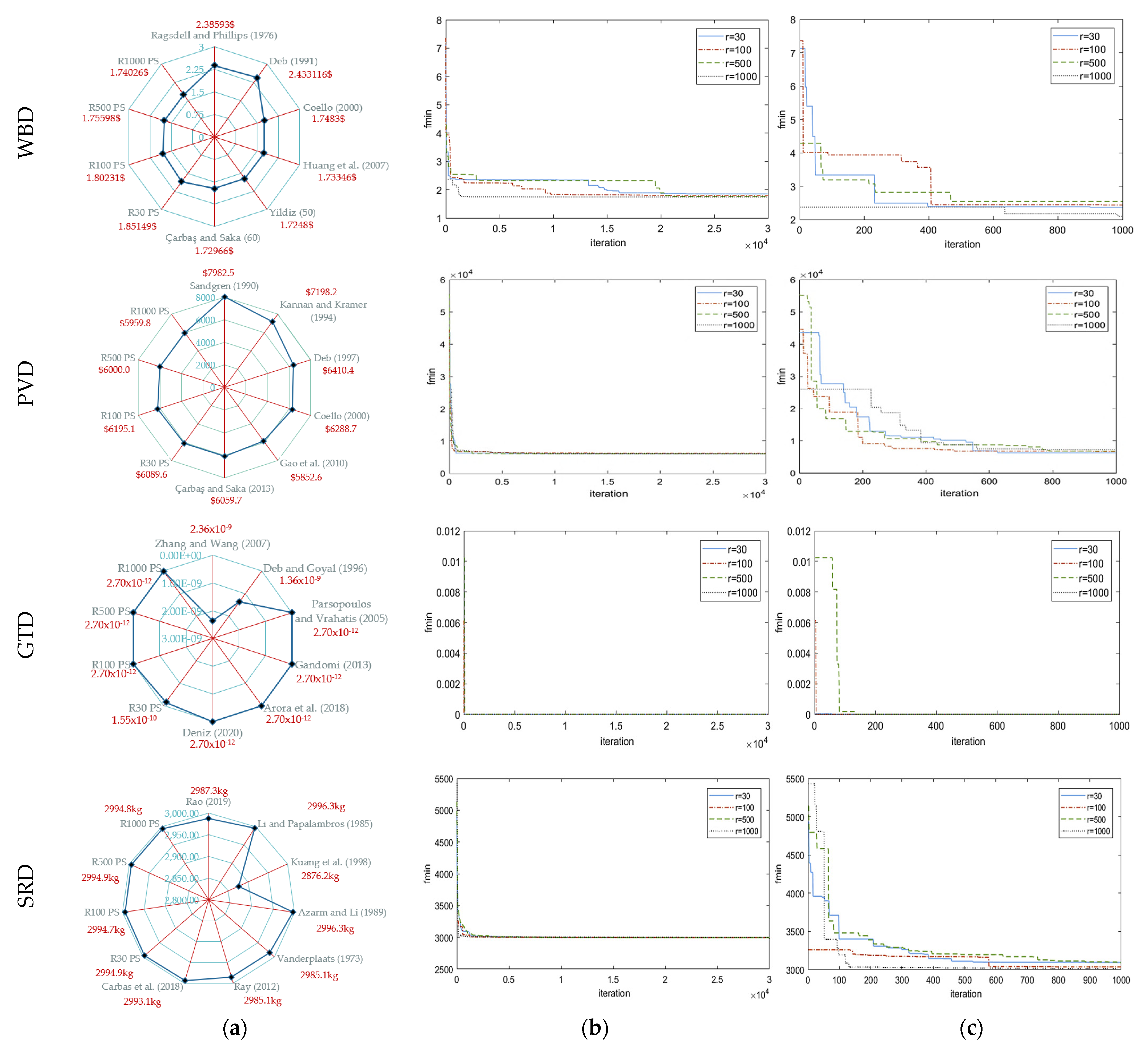
2.1.1. Welded Beam Design Problem
2.1.2. Pressure Vessel Design Problem
2.1.3. Gear Train Design
2.1.4. Speed Reducer Design
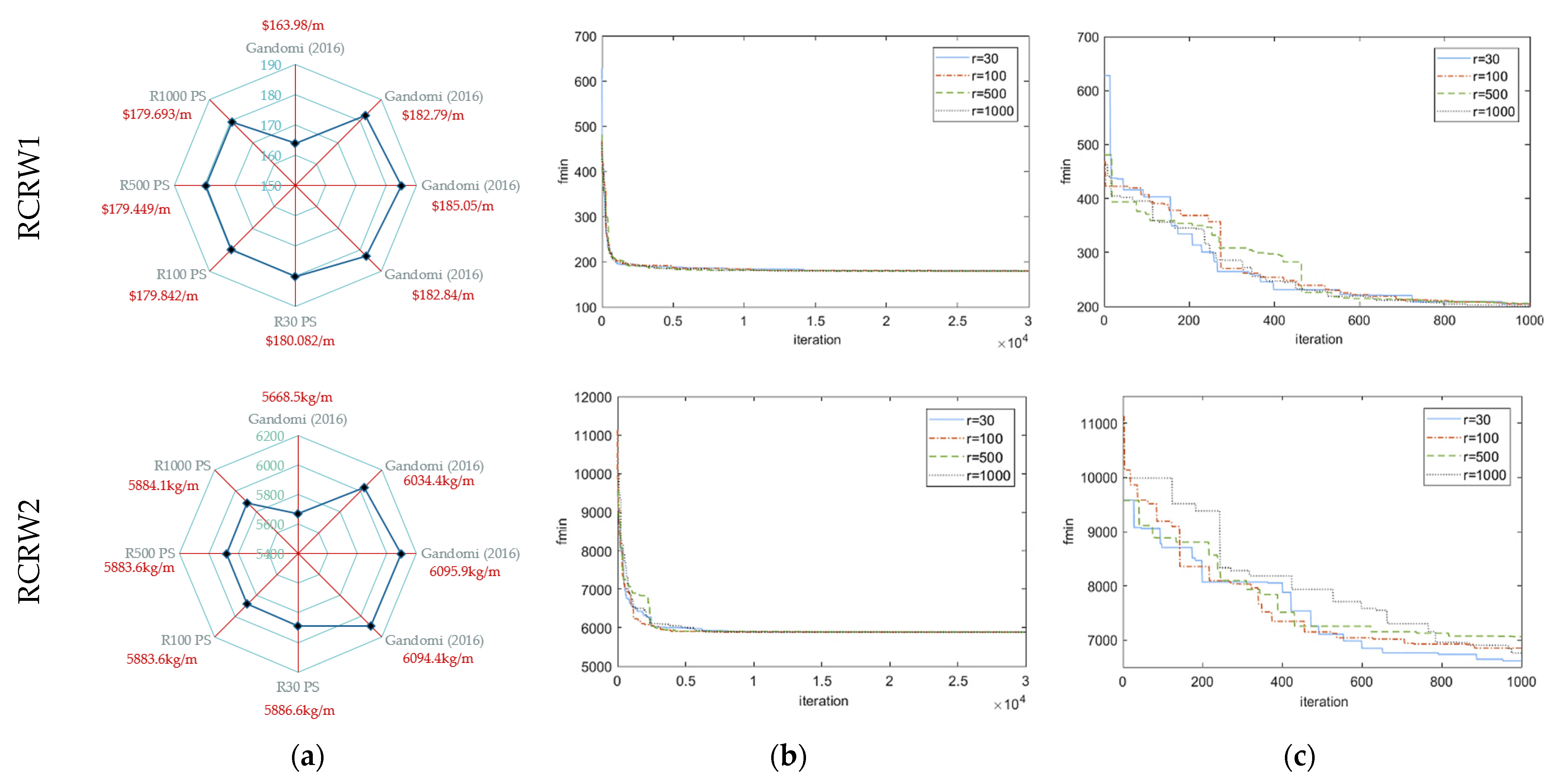
2.2. Real-Size Engineering Design Optimization Problem

| Input Parameters | Symbol | Value | Unit |
|---|---|---|---|
| Stem height | H | 4.5 | m |
| Surcharge load | q | 30 | kPa |
| Backfill slope | β | 0 | ° |
| Internal friction angle of the retained soil and the base soil | Ør and Øb | 36 and 34 | ° |
| Unit weight of retained soil, base soil, and concrete | γr, γb, and γc | 17.5, 18.5, 23.5 | kPa |
| Cohesion of base and retained soils | cb and cr | 0 | kPa |
| Depth of soil in front of the wall | Df | 0.75 | m |
| Terzaghi bearing capacity factors for Øb = 34° [45] | Nc, Nq, Nγ | 52.64, 36.50, 38.04 | – |
| The factor of safety for sliding and overturning stability | SFss and SFso | 1.50 | – |
| The factor of safety for bearing capacity | SFsb | 3.00 | – |
| Reinforcing steel yield strength | fy | 400 | MPa |
| Concrete compressive strength | fc | 21 | MPa |
| Concrete cover | cc | 0.07 | m |
| Shrinkage and temperature reinforcement percentage | ρst | 0.002 | – |
| Nominal strength coefficient for the flexural moment | ϕm | 0.90 | – |
| Nominal strength coefficient for shear force | ϕ | 0.75 | – |
| Reinforcement location factor (1.0 for concrete below < 30.48 cm) | ψt | 1.00 | – |
| Coating factor (for uncoated bars) | ψe | 1.00 | – |
| Lightweight aggregate concrete factor (1.0 for normal-weight conc.) | λ | 1.00 | – |
| Cost of steel and concrete | Cs and Cc | 0.4 and 40 | $/kg and $/m3 |
2.3. Harmony Search Algorithm
- Step 1: HSA is initialized by determining the constant algorithm parameters (HMS, HMCR, PAR, and maximum iteration number) and generating design space with design variable values according to range limitation;
- Step 2: HM matrix is formed randomly by selecting from design space;
- Step 3: Improvisation of a new HM matrix conceiving memory consideration, random selection, and pitch adjustment mechanisms is carried out;
- Step 4: HM matrix is updated depending on whether a better solution is obtained, and then the worst solution is drawn from HM by replacing the better one;
- Step 5: Until the current iteration is reached the predefined maximum iteration number, Step 3 and Step 4 are repeated. If it is conducted HSA is ended.
2.4. Taguchi Method Background
2.5. A New Hybrid Method Based on Taguchi for Optimum Values of Algorithm Parameters
2.5.1. Forming Taguchi Design Matrix
2.5.2. Initializing HSA Process
2.5.3. Performing Taguchi Analyses
3. Design Experiments and Results
3.1. Optimization Analyses of Engineering Design Problems and Real-Size Engineering Design Optimization Problem
3.2. Taguchi Analyses
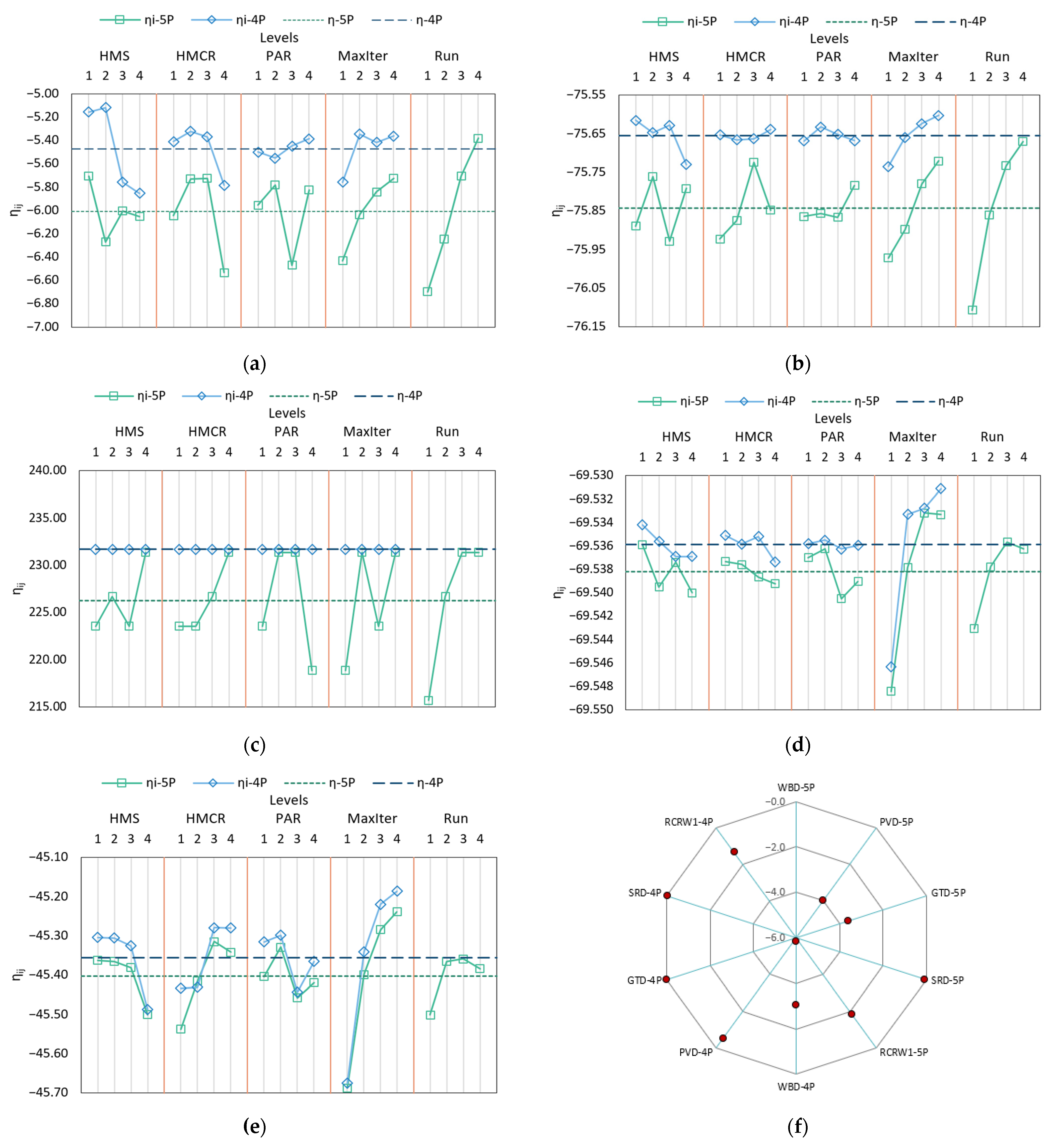
3.2.1. Part I: Investigation of Five Optimum Design Parameter Values with Effect on the Fitness Value
3.2.2. Part II: Investigation of Four Optimum Design Parameter Values with Effect on the Fitness Value
4. Discussion
5. Conclusions
- The obtained estimations have a reasonable relative error in determining optimum values of algorithm design parameters without performing many trials;
- It has been seen that the optimum values of the algorithm design parameters vary depending on the nature of the design optimization problem, which includes the number of design variables, the number of design constraints, exposure to the constraints.
- Instead of taking into account the value of the algorithm parameter proposed for characteristically different optimization problems in the literature, it has been concluded that using the optimum values yielded statistically according to the nature of the problem is an effective and prosperous manner in converging to the optimum.
- Instead of the trial-error method, which is time-consuming and exhaustive, it has been concluded that the newly proposed TIHHSA is a robust and reliable method for estimating the optimum algorithm parameter values of the harmony search metaheuristic optimization technique in a shorter time without conducting sensitivity analyses which are utilized to increase convergence rate in the solution of the design optimization problem.
Author Contributions
Funding
Institutional Review Board Statement
Informed Consent Statement
Data Availability Statement
Conflicts of Interest
Appendix A
| Optimum Solutions | x1(h)(in.) | x2(l) (in.) | x3(t) (in.) | x4(b) (in.) | f(x) ($) | |
|---|---|---|---|---|---|---|
| Literature | Ragsdell and Phillips [50] | 0.24550 | 6.1960 | 8.2730 | 0.2455 | 2.38593 |
| Deb [51] | 0.2489 | 6.173 | 8.1789 | 0.2533 | 2.433116 | |
| Coello [52] | 0.2088 | 3.4205 | 8.9975 | 0.21 | 1.7483 | |
| Huang et al. [53] | 0.203137 | 3.542998 | 9.033498 | 0.206179 | 1.73346 | |
| Yildiz [54] | 0.20573 | 3.47042 | 9.03649 | 0.205735 | 1.7248 | |
| Çarbaş and Saka [55] | 0.203907 | 3.499898 | 9.063898 | 0.205594 | 1.72966 | |
| Case PS | R30 | 0.206741 | 3.65285 | 8.54856 | 0.231265 | 1.85149 |
| R100 | 0.171535 | 4.42418 | 8.98313 | 0.208289 | 1.80231 | |
| R500 | 0.198864 | 3.66442 | 8.94678 | 0.209895 | 1.75598 | |
| R1000 | 0.19823 | 3.64539 | 9.02857 | 0.206407 | 1.74026 | |
| WBD-5P | 0.195872 | 3.70387 | 9.07235 | 0.205574 | 1.7455 | |
| WBD-4P | 0.188171 | 3.95948 | 8.91723 | 0.21133 | 1.78312 | |
| Optimum Solutions | x1(Ts) (in.) | x2(Th) (in.) | x3(R) (in.) | x4(L) (in.) | f(x) ($) | |
|---|---|---|---|---|---|---|
| Literature | Sandgren [35] | 1.125 | 0.625 | 48.97 | 106.72 | 7982.5 |
| Kannan and Kramer [56] | 1.25 | 0.625 | 50 | 120 | 7198.20 | |
| Deb [57] | 0.9375 | 0.50 | 48.329 | 112.679 | 6410.381 | |
| Coello [52] | 0.8125 | 0.4375 | 40.3239 | 200.0 | 6288.7445 | |
| Gao et al. [58] | 0.75 | 0.375 | 38.8441 | 221.612 | 5852.639 | |
| Çarbaş and Saka [55] | 0.8125 | 0.4375 | 42.09845 | 176.6366 | 6059.7143 | |
| Case PS | R30 | 0.876366 | 0.434563 | 45.3293 | 140.344 | 6089.66 |
| R100 | 0.915835 | 0.454142 | 47.2497 | 121.872 | 6195.1 | |
| R500 | 0.833985 | 0.413952 | 43.1577 | 163.94 | 6000.09 | |
| R1000 | 0.814181 | 0.403799 | 42.1533 | 176.032 | 5959.86 | |
| PVD-5P | 0.84119 | 0.430252 | 43.5749 | 159.245 | 6054.14 | |
| PVD-4P | 0.822121 | 0.409189 | 42.367 | 173.44 | 6005.19 | |
| Optimum Solutions | x1(Ta) (piece) | x2(Tb) (piece) | x3(Td) (piece) | x4 (Tf) (piece) | Gear ratio | f(x) (unitless) | |
|---|---|---|---|---|---|---|---|
| Literature | Zhang and Wang [59] | 43 | 16 | 19 | 49 | 0.1442 | 2.36 × 10⁻⁹ |
| Deb and Goyal [60] | 33 | 14 | 17 | 50 | 0.1442 | 1.362 × 10⁻⁹ | |
| Parsopoulos and Vrahatis [61] | 43 | 16 | 19 | 49 | 0.1442 | 2.701 × 10⁻¹² | |
| Gandomi [62] | 43 | 16 | 19 | 49 | 0.1442 | 2.701 × 10⁻¹² | |
| Arora et al. [63] | 43 | 16 | 19 | 49 | 0.1442 | 2.701 × 10⁻¹² | |
| Deniz [64] | 43 | 16 | 19 | 49 | 0.1442 | 2.701 × 10⁻¹² | |
| Case PS | R30 | 44 | 13 | 21 | 43 | 0.144292 | 1.54505 × 10⁻¹⁰ |
| R100 | 43 | 16 | 19 | 49 | 0.144281 | 2.70086 × 10⁻¹² | |
| R500 | 49 | 16 | 19 | 43 | 0.144281 | 2.70086 × 10⁻¹² | |
| R1000 | 49 | 16 | 19 | 43 | 0.144281 | 2.70086 × 10⁻¹² | |
| GTD-5P | 49 | 16 | 19 | 43 | 0.144281 | 2.70086 × 10⁻¹² | |
| GTD-4P | 49 | 16 | 19 | 43 | 0.144281 | 2.70086 × 10⁻¹² | |
| Optimum Solutions | x1 (cm) | x2 (cm) | x3 (piece) | x4 (cm) | x5 (cm) | x6 (cm) | x7 (cm) | f(x) (kg) | |
|---|---|---|---|---|---|---|---|---|---|
| Literature | Li and Papalambros [65] | 3.50 | 0.70 | 17.00 | 7.30 | 7.71 | 3.3500000 | 5.2900000 | 2996.30977 |
| Kuang et al. [66] | 3.60 | 0.70 | 17.00 | 7.30 | 7.80 | 3.4000000 | 5.0000000 | 2876.22 | |
| Azarm and Li [67] | 3.50 | 0.70 | 17.00 | 7.30 | 7.71 | 3.3500000 | 5.2900000 | 2996.30978 | |
| Vanderplaats [68] | 3.50 | 0.70 | 17.00 | 7.30 | 7.30 | 3.3502145 | 5.2865176 | 2985.15188 | |
| Ray [69] | 3.50 | 0.70 | 17.00 | 7.30 | 7.30 | 3.3502145 | 5.2865176 | 2985.15188 | |
| Carbas et al. [70] | 3.50 | 0.70 | 17.00 | 7.17984 | 7.70889 | 3.35009 | 5.28668 | 2993.13917 | |
| Case PS | R30 | 3.5001 | 0.700016 | 17.0017 | 7.30052 | 7.71562 | 3.35025 | 5.28667 | 2994.93 |
| R100 | 3.50014 | 0.700021 | 17.0002 | 7.30117 | 7.71637 | 3.35053 | 5.28667 | 2994.79 | |
| R500 | 3.50029 | 0.700019 | 17.0001 | 7.3009 | 7.71572 | 3.35053 | 5.28681 | 2994.90 | |
| R1000 | 3.50025 | 0.700016 | 17.0004 | 7.30034 | 7.71652 | 3.35036 | 5.28673 | 2994.84 | |
| SRD-5P | 3.50184 | 0.700073 | 17.0008 | 7.3036 | 7.72133 | 3.35036 | 5.28679 | 2995.97 | |
| SRD-4P | 3.50006 | 0.700006 | 17.0034 | 7.30108 | 7.71868 | 3.3516 | 5.28677 | 2995.63 | |
| R30 | R100 | R500 | R1000 | 5P | 4P | R30 | R100 | R500 | R1000 | 5P | 4P | ||||
|---|---|---|---|---|---|---|---|---|---|---|---|---|---|---|---|
| WBD | g1(x) | −8.821 | −0.086 | −7.948 | −7.525 | −65.745 | −32.706 | SRD | g1(x) | 0.92592 | 0.92598 | 0.92595 | 0.92595 | 0.92536 | 0.92587 |
| g2(x) | −178.142 | −14.670 | −1.819 | −45.079 | −213.275 | −7.722 | g2(x) | 0.80178 | 0.80190 | 0.80188 | 0.80187 | 0.80134 | 0.80165 | ||
| g3(x) | −0.025 | −0.037 | −0.011 | −0.008 | −0.010 | −0.023 | g3(x) | 0.50085 | 0.50086 | 0.50081 | 0.50079 | 0.50141 | 0.50012 | ||
| g4(x) | −3.317 | −3.338 | −3.400 | −3.414 | −3.407 | −3.368 | g4(x) | 0.09535 | 0.09539 | 0.09536 | 0.09539 | 0.09555 | 0.09545 | ||
| g5(x) | −0.082 | −0.047 | −0.074 | −0.073 | −0.071 | −0.063 | g5(x) | 0.99994 | 0.99944 | 0.99944 | 0.99974 | 0.99975 | 0.99752 | ||
| g6(x) | −0.235 | −0.235 | −0.235 | −0.236 | −0.236 | −0.235 | g6(x) | 0.99998 | 0.99998 | 0.99982 | 0.99991 | 0.99985 | 0.99987 | ||
| g7(x) | −2211.802 | −202.416 | −330.005 | −55.908 | −1.921 | −446.574 | g7(x) | 0.29754 | 0.29751 | 0.29751 | 0.29751 | 0.29755 | 0.29756 | ||
| PVD | g1(x) | −0.002 | −0.002 | −0.004 | −0.001 | −0.001 | 0.000 | g8(x) | 0.99999 | 0.99999 | 0.99994 | 0.99995 | 0.99958 | 0.99999 | |
| g2(x) | −0.002 | −0.002 | −0.003 | −0.002 | −0.002 | −0.015 | g9(x) | 0.41667 | 0.41667 | 0.41669 | 0.41669 | 0.41684 | 0.41667 | ||
| g3(x) | −89.466 | −89.466 | −636.323 | −9.038 | −412.835 | −498.618 | g10(x) | 0.94861 | 0.94859 | 0.94862 | 0.94866 | 0.94824 | 0.94882 | ||
| g4(x) | −99.656 | −99.656 | −118.128 | −76.060 | −63.968 | −80.755 | g11(x) | 0.99996 | 0.99987 | 0.99997 | 0.99986 | 0.99924 | 0.99958 |
| Optimum Solutions | x1 (m) | x2 (m) | x3 (m) | x4 (m) | x5 (m) | x6 (m) | x7 (m) | x8 (cm2) | x9 (cm2) | x10 (cm2) | x11 (cm2) | x12 (cm2) | f(x) ($/kg) | |
|---|---|---|---|---|---|---|---|---|---|---|---|---|---|---|
| Literature | Gandomi [40] | 2.709 | 1 | 0.412 | 0.25 | 0.4 | 2.455 | 0.2 | 0.2 | 21.9911 | 11.7809 | 11.7809 | 4.7124 | 163.98 |
| Gandomi [40] | 2.727 | 1.035 | 0.36 | 0.28 | 0.401 | 2.274 | 0.293 | 0.296 | 32.1699 | 13.3517 | 13.8544 | 8.6394 | 182.79 | |
| Gandomi [40] | 2.816 | 0.988 | 0.447 | 0.294 | 0.422 | 2.223 | 0.367 | 0.203 | 21.9911 | 15.2681 | 15.2681 | 12.7234 | 185.05 | |
| Gandomi [40] | 2.694 | 0.836 | 0.403 | 0.27 | 0.405 | 2.346 | 0.227 | 0.445 | 23.7504 | 12.7234 | 22.6195 | 26.1380 | 182.84 | |
| CasePS | R30 | 3.3439 | 1.1598 | 0.3526 | 0.2504 | 0.4 | 2.5435 | 0.2002 | 0.2 | 21.2999 | 14.3212 | 18.8016 | 7.1532 | 180.082 |
| R100 | 3.3431 | 1.1596 | 0.3917 | 0.25 | 0.4001 | 2.4623 | 0.2001 | 0.2002 | 18.8963 | 14.2586 | 18.9194 | 9.5172 | 179.842 | |
| R500 | 3.3351 | 1.1593 | 0.4418 | 0.25 | 0.4001 | 3.0523 | 0.2004 | 0.2002 | 16.6776 | 14.3189 | 16.557 | 7.2319 | 179.449 | |
| R1000 | 3.3394 | 1.1593 | 0.3916 | 0.2501 | 0.4 | 2.7275 | 0.2004 | 0.2003 | 18.691 | 14.392 | 18.7638 | 7.2583 | 179.693 | |
| RCRW1−5P | 3.36761 | 1.15955 | 0.391877 | 0.250366 | 0.400094 | 2.84595 | 0.200248 | 0.201545 | 18.7689 | 14.4128 | 18.7273 | 10.0995 | 181.035 | |
| RCRW1−4P | 3.34757 | 1.15992 | 0.394711 | 0.250081 | 0.400157 | 2.37294 | 0.202173 | 0.201494 | 18.7718 | 14.1765 | 18.7523 | 9.34978 | 180.301 | |
| Optimum Solutions | x1 (m) | x2 (m) | x3 (m) | x4 (m) | x5 (m) | x6 (m) | x7 (m) | x8 (cm2) | x9 (cm2) | x10 (cm2) | x11 (cm2) | x12 (cm2) | f(x) ($/kg) | |
|---|---|---|---|---|---|---|---|---|---|---|---|---|---|---|
| Literature | Gandomi [40] | 2.709 | 1 | 0.412 | 0.25 | 0.4 | 2.455 | 0.2 | 0.2 | 21.9911 | 11.7809 | 11.7809 | 4.7124 | 5668.5 |
| Gandomi [40] | 2.727 | 1.035 | 0.36 | 0.28 | 0.401 | 2.274 | 0.293 | 0.296 | 32.1699 | 13.3517 | 13.8544 | 8.6394 | 6034.4 | |
| Gandomi [40] | 2.816 | 0.988 | 0.447 | 0.294 | 0.422 | 2.223 | 0.367 | 0.203 | 21.9911 | 15.2681 | 15.2681 | 12.7234 | 6095.9 | |
| Gandomi [40] | 2.694 | 0.836 | 0.403 | 0.27 | 0.405 | 2.346 | 0.227 | 0.445 | 23.7504 | 12.7234 | 22.6195 | 26.1380 | 6094.4 | |
| CasePS | R30 | 3.342 | 1.1599 | 0.2505 | 0.2504 | 0.4 | 3.1292 | 0.2001 | 0.2001 | 35.1479 | 14.1715 | 21.5672 | 7.0299 | 5886.67 |
| R100 | 3.3426 | 1.16 | 0.2501 | 0.2501 | 0.4 | 3.0709 | 0.2001 | 0.2002 | 35.1127 | 15.0607 | 21.2321 | 7.0677 | 5883.61 | |
| R500 | 3.343 | 1.1581 | 0.25 | 0.25 | 0.4001 | 3.0355 | 0.2001 | 0.2002 | 35.247 | 14.4184 | 21.3267 | 7.3429 | 5883.64 | |
| R1000 | 3.3434 | 1.1594 | 0.2501 | 0.25 | 0.4 | 3.1304 | 0.2001 | 0.2001 | 35.2741 | 14.1095 | 21.2558 | 9.3741 | 5884.09 | |
| RCRW1−5P | 2.709 | 1 | 0.412 | 0.25 | 0.4 | 2.455 | 0.2 | 0.2 | 21.9911 | 11.7809 | 11.7809 | 4.7124 | 5668.5 | |
| RCRW1−4P | 2.727 | 1.035 | 0.36 | 0.28 | 0.401 | 2.274 | 0.293 | 0.296 | 32.1699 | 13.3517 | 13.8544 | 8.6394 | 6034.4 | |
| Optimum Cost (RCRW1) | Optimum Weight (RCRW2) | |||||||||
|---|---|---|---|---|---|---|---|---|---|---|
| R30 | R100 | R500 | R1000 | 5P | 4P | R30 | R100 | R500 | R1000 | |
| g1(x) | −0.0462 | −0.043 | −0.037 | −0.0421 | −0.0497 | −0.0441 | −0.0536 | −0.0537 | −0.0543 | −0.0541 |
| g2(x) | −0.638 | −0.6334 | −0.6224 | −0.6305 | −0.6613 | −0.6376 | −0.6468 | −0.6472 | −0.648 | −0.6484 |
| g3(x) | −2.5539 | −2.569 | −2.5824 | −2.5638 | −2.6425 | −2.5813 | −2.5106 | −2.5112 | −2.5092 | −2.5137 |
| g4(x) | −0.1129 | −0.1141 | −0.0221 | −0.0199 | −1.8384 | −0.3677 | −0.0072 | −0.0142 | −0.0149 | −0.0925 |
| g5(x) | −0.0001 | −0.0004 | 0.0000 | −0.0002 | −0.0009 | −0.0085 | −0.0633 | −0.0615 | −0.061 | −0.0615 |
| g6(x) | −0.4023 | −0.4058 | −0.4103 | −0.4057 | −0.4115 | −0.4066 | −0.3937 | −0.4242 | −0.3951 | −0.3944 |
| g7(x) | −0.0326 | −0.0701 | −0.0052 | −0.0728 | −0.0531 | −0.07 | −0.062 | −0.0482 | −0.0464 | −0.0472 |
| g8(x) | −0.9964 | −0.9973 | −0.9964 | −0.9964 | −0.9974 | −0.9973 | −0.9964 | −0.9964 | −0.9964 | −0.9973 |
| g9(x) | −0.3955 | −0.4637 | −0.5333 | −0.4635 | −0.464 | −0.4684 | −0.1169 | −0.1154 | −0.115 | −0.1154 |
| g10(x) | −0.4032 | −0.4065 | −0.4107 | −0.4064 | −0.4096 | −0.407 | −0.3956 | −0.3955 | −0.3964 | −0.3959 |
| g11(x) | −0.065 | −0.0845 | −0.1132 | −0.0858 | −0.0767 | −0.0847 | −0.0179 | −0.0175 | −0.0167 | −0.017 |
| g12(x) | −0.9936 | −0.9935 | −0.9936 | −0.9935 | −0.9934 | −0.9936 | −0.9935 | −0.9935 | −0.9935 | −0.9935 |
| g13(x) | −0.4189 | −0.2727 | −0.0625 | −0.2729 | −0.2724 | −0.2671 | −0.7519 | −0.7523 | −0.7524 | −0.7523 |
| g14(x) | −0.0097 | −0.0095 | −0.0095 | −0.0097 | −0.0095 | −0.0093 | −0.0097 | −0.0618 | −0.0095 | −0.0097 |
| g15(x) | −0.2573 | −0.2571 | −0.151 | −0.2573 | −0.2571 | −0.257 | −0.3504 | −0.3408 | −0.3406 | −0.3408 |
| g16(x) | −0.0087 | −0.2569 | −0.0077 | −0.0077 | −0.3028 | −0.2492 | −0.0092 | −0.0092 | −0.0092 | −0.2569 |
| g17(x) | −0.6471 | −0.7181 | −0.7813 | −0.718 | −0.7182 | −0.7202 | −0.1734 | −0.1721 | −0.1718 | −0.1721 |
| g18(x) | −0.7929 | −0.793 | −0.793 | −0.7929 | −0.793 | −0.793 | −0.7929 | −0.7814 | −0.793 | −0.7929 |
| g19(x) | −0.7239 | −0.724 | −0.7585 | −0.7239 | −0.724 | −0.724 | −0.6844 | −0.689 | −0.689 | −0.689 |
| g20(x) | −0.7931 | −0.7241 | −0.7934 | −0.7934 | −0.7059 | −0.7269 | −0.793 | −0.793 | −0.793 | −0.7241 |
| g21(x) | −0.5477 | −0.536 | −0.5199 | −0.5356 | −0.5393 | −0.5356 | −0.578 | −0.5781 | −0.5788 | −0.5784 |
| g22(x) | −0.1795 | −0.2036 | −0.0247 | −0.1232 | −0.0954 | −0.2308 | −0.0038 | −0.0214 | −0.0321 | −0.0039 |
| g23(x) | −0.2382 | −0.3654 | −0.3654 | −0.3652 | −0.3654 | −0.3655 | −0.3652 | −0.3652 | −0.3654 | −0.3652 |
| g24(x) | −0.6364 | −0.6365 | −0.6365 | −0.6364 | −0.6365 | −0.6365 | −0.6364 | −0.4909 | −0.6365 | −0.6364 |
| g25(x) | −0.6364 | −0.6365 | −0.6365 | −0.6364 | −0.6365 | −0.6365 | −0.4182 | −0.5636 | −0.5638 | −0.5636 |
| g26(x) | −0.1113 | −0.3654 | −0.1115 | −0.1113 | −0.1115 | −0.3655 | −0.1113 | −0.1113 | −0.1115 | −0.3652 |
References
- Houssein, E.H.; Mahdy, M.A.; Shebl, D.; Mohamed, W.M. A Survey of Metaheuristic Algorithms for Solving Optimization Problems. Stud. Comput. Intell. 2021, 967, 515–543. [Google Scholar] [CrossRef]
- Dubey, M.; Kumar, V.; Kaur, M.; Dao, T.P. A Systematic Review on Harmony Search Algorithm: Theory, Literature, and Applications. Math. Probl. Eng. 2021, 2021, 5594267. [Google Scholar] [CrossRef]
- Dorigo, M.; Gambardella, L.M. Ant Colonies for the Travelling Salesman Problem. BioSystems 1997, 43, 73–81. [Google Scholar] [CrossRef] [Green Version]
- Kennedy, J.; Eberhart, R. Particle Swarm Optimization. In Proceedings of the ICNN’95—International Conference on Neural Networks, Perth, WA, Australia, 27 November–1 December 1995; IEEE: Piscataway, NJ, USA, 1995; Volume 4, pp. 1942–1948. [Google Scholar]
- Karaboga, D. An Idea Based on Honey Bee Swarm for Numerical Optimization; Technical Report TR06; Erciyes University: Kayseri, Turkey, 2005. [Google Scholar]
- Mirjalili, S.; Lewis, A. The Whale Optimization Algorithm. Adv. Eng. Softw. 2016, 95, 51–67. [Google Scholar] [CrossRef]
- Rashedi, E.; Nezamabadi-pour, H.; Saryazdi, S. GSA: A Gravitational Search Algorithm. Inf. Sci. 2009, 179, 2232–2248. [Google Scholar] [CrossRef]
- Erol, O.K.; Eksin, I. A New Optimization Method: Big Bang–Big Crunch. Adv. Eng. Softw. 2006, 37, 106–111. [Google Scholar] [CrossRef]
- Rajabioun, R. Cuckoo Optimization Algorithm. Appl. Soft Comput. 2011, 11, 5508–5518. [Google Scholar] [CrossRef]
- Yang, X.S. Firefly Algorithms for Multimodal Optimization. In International Symposium on Stochastic Algorithms. SAGA 2009: Stochastic Algorithms: Foundations and Applications; Watanabe, O., Zeugmann, T., Eds.; Lecture Notes in Computer Science; Springer: Berlin/Heidelberg, Germany, 2009; Volume 5792, pp. 169–178. ISBN 978-3-642-04943-9. [Google Scholar] [CrossRef] [Green Version]
- Yang, X.-S. A New Metaheuristic Bat-Inspired Algorithm. In Nature Inspired Cooperative Strategies for Optimization; González, J.R., Pelta, D.A., Cruz, C., Terrazas, G., Natalio, K., Eds.; Springer: Berlin/Heidelberg, Germany, 2010; Volume 284, pp. 65–74. [Google Scholar]
- Storn, R.; Price, K. Differential Evolution—A Simple and Efficient Heuristic for Global Optimization over Continuous Spaces. J. Glob. Optim. 1997, 11, 341–359. [Google Scholar] [CrossRef]
- Simon, D. Biogeography-Based Optimization. IEEE Trans. Evol. Comput. 2008, 12, 702–713. [Google Scholar] [CrossRef] [Green Version]
- Goldberg, D.E.; Kuo, C.H. Genetic Algorithms in Pipeline Optimization. J. Comput. Civ. Eng. 1987, 1, 128–141. [Google Scholar] [CrossRef]
- Kirkpatrick, S.; Gelatt, C.D.; Vecchi, M.P. Optimization by Simulated Annealing. Science 1983, 220, 671–680. [Google Scholar] [CrossRef]
- Geem, Z.W.; Kim, J.H.; Loganathan, G.V. A New Heuristic Optimization Algorithm: Harmony Search. Simulation 2001, 76, 60–68. [Google Scholar] [CrossRef]
- Hakli, H.; Ortacay, Z. An Improved Scatter Search Algorithm for the Uncapacitated Facility Location Problem. Comput. Ind. Eng. 2019, 135, 855–867. [Google Scholar] [CrossRef]
- Mahdavi, M.; Fesanghary, M.; Damangir, E. An Improved Harmony Search Algorithm for Solving Optimization Problems. Appl. Math. Comput. 2007, 188, 1567–1579. [Google Scholar] [CrossRef]
- Liu, Y. Hybrid Particle Swarm Optimizer for Constrained Optimization Problems. Qinghua Daxue Xuebao/J. Tsinghua Univ. 2013, 53, 242–246. [Google Scholar]
- Fesanghary, M.; Mahdavi, M.; Minary-Jolandan, M.; Alizadeh, Y. Hybridizing Harmony Search Algorithm with Sequential Quadratic Programming for Engineering Optimization Problems. Comput. Methods Appl. Mech. Eng. 2008, 197, 3080–3091. [Google Scholar] [CrossRef]
- Sheikholeslami, R.; Khalili, B.G.; Sadollah, A.; Kim, J.H. Optimization of Reinforced Concrete Retaining Walls via Hybrid Firefly Algorithm with Upper Bound Strategy. KSCE J. Civ. Eng. 2016, 20, 2428–2438. [Google Scholar] [CrossRef]
- Search for Hybrid Optimization in Web of Science. Available online: https://www.webofscience.com/wos/woscc/summary/19ecf7e7-1092-459a-bc98-e94ff827d659-0de1a535/relevance/1 (accessed on 22 October 2021).
- Search for Hybrid Harmony Search in Web of Science. Available online: https://www.webofscience.com/wos/woscc/summary/f92b392b-51ef-41e5-9784-2f785de062f3-0f0bc6d0/relevance/1 (accessed on 22 October 2021).
- Akay, B.; Karaboga, D. A Modified Artificial Bee Colony Algorithm for Real-Parameter Optimization. Inf. Sci. 2012, 192, 120–142. [Google Scholar] [CrossRef]
- Uray, E.; Hakli, H.; Carbas, S. Statistical Investigation of the Robustness for the Optimization Algorithms. In Nature-Inspired Metaheuristic Algorithms for Engineering Optimization Applications; Carbas, S., Toktas, A., Ustun, D., Eds.; Springer: Singapore, 2021; pp. 201–224. [Google Scholar]
- Taguchi, G. Introduction to Quality Engineering: Designing Quality into Products and Processes; The Organization: Tokyo, Japan, 1986; ISBN 9283310837. [Google Scholar]
- Taguchi, G.; Chowdhury, S.; Wu, Y. Taguchi’s Quality Engineering Handbook; John Wiley & Sons, Inc.: Hoboken, NJ, USA, 2005; ISBN 9780471413349. [Google Scholar]
- Chao, S.-M.; Whang, A.J.-W.; Chou, C.-H.; Su, W.-S.; Hsieh, T.-H. Optimization of a Total Internal Reflection Lens by Using a Hybrid Taguchi-Simulated Annealing Algorithm. Opt. Rev. 2014, 21, 153–161. [Google Scholar] [CrossRef]
- Tsai, J.; Liu, T.; Chou, J. Hybrid Taguchi-Genetic Algorithm for Global Numerical Optimization. IEEE Trans. Evol. Comput. 2004, 8, 365–377. [Google Scholar] [CrossRef]
- Cheng, B.W.; Chang, C.L. A Study on Flowshop Scheduling Problem Combining Taguchi Experimental Design and Genetic Algorithm. Expert Syst. Appl. 2007, 32, 415–421. [Google Scholar] [CrossRef]
- Jia, X.; Lu, G. A Hybrid Taguchi Binary Particle Swarm Optimization for Antenna Designs. IEEE Antennas Wirel. Propag. Lett. 2019, 18, 1581–1585. [Google Scholar] [CrossRef]
- Yildiz, A.R.; Öztürk, F. Hybrid Taguchi-Harmony Search Approach for Shape Optimization. Stud. Comput. Intell. 2010, 270, 89–98. [Google Scholar] [CrossRef]
- Uray, E.; Tan, Ö.; Çarbaş, S.; Erkan, H. Metaheuristics-Based Pre-Design Guide for Cantilever Retaining Walls. Tek. Dergi 2021, 32, 10967–10993. [Google Scholar] [CrossRef] [Green Version]
- Rao, S. Engineering Optimization: Theory and Practice; John Wiley & Sons: Hoboken, NJ, USA, 1996. [Google Scholar]
- Sandgren, E. Nonlinear Integer and Discrete Programming in Mechanical Design Optimization. J. Mech. Des. 1990, 112, 223–229. [Google Scholar] [CrossRef]
- Jan Golinski Optimal Synthesis Problems Solved by Means of Nonlinear Programming and Random Methods. J. Mech. 1970, 5, 287–309. [CrossRef]
- Afzal, M.; Liu, Y.; Cheng, J.C.P.; Gan, V.J.L. Reinforced Concrete Structural Design Optimization: A Critical Review. J. Clean. Prod. 2020, 260, 120623. [Google Scholar] [CrossRef]
- ACI Committee. Building Code Requirements for Structural Concrete (ACI 318-05) and Commentary (ACI 318R-05); American Concrete Institute: Farmington Hills, MI, USA, 2005. [Google Scholar]
- Akin, A.; Saka, M.P. Optimum Design of Concrete Cantilever Retaining Walls Using the Harmony Search Algorithm. Civ. -Comp Proc. 2010, 93, 1–21. [Google Scholar] [CrossRef]
- Gandomi, A.H.; Kashani, A.R.; Roke, D.A.; Mousavi, M. Optimization of Retaining Wall Design Using Evolutionary Algorithms. Struct. Multidiscip. Optim. 2016, 55, 809–825. [Google Scholar] [CrossRef]
- Kalemci, E.N.; İkizler, S.B.; Dede, T.; Angın, Z. Design of Reinforced Concrete Cantilever Retaining Wall Using Grey Wolf Optimization Algorithm. Structures 2020, 23, 245–253. [Google Scholar] [CrossRef]
- Uray, E.; Çarbaş, S.; Erkan, İ.H.; Tan, Ö. Parametric Investigation for Discrete Optimal Design of a Cantilever Retaining Wall. Chall. J. Struct. Mech. 2019, 5, 108. [Google Scholar] [CrossRef]
- Uray, E.; Çarbaş, S.; Erkan, İ.H.; Olgun, M. Investigation of Optimal Designs for Concrete Cantilever Retaining Walls in Different Soils. Chall. J. Concr. Res. Lett. 2020, 11, 39. [Google Scholar] [CrossRef]
- Camp, C.; Akin, A. Design of Retaining Walls Using Big Bang–Big Crunch Optimization. J. Struct. Eng. 2012, 138, 438–448. [Google Scholar] [CrossRef]
- Das, B.M.; Sivakugan, N. Principles of Foundation Engineering, 9th ed.; Cengage Learning: Boston, MA, USA, 2017; ISBN 9781305970953. [Google Scholar]
- Gandomi, A.H.; Kashani, A.R.; Roke, D.A.; Mousavi, M. Optimization of Retaining Wall Design Using Recent Swarm Intelligence Techniques. Eng. Struct. 2015, 103, 72–84. [Google Scholar] [CrossRef]
- Lee, K.S.; Geem, Z.W. A New Meta-Heuristic Algorithm for Continuous Engineering Optimization: Harmony Search Theory and Practice. Comput. Methods Appl. Mech. Eng. 2005, 194, 3902–3933. [Google Scholar] [CrossRef]
- Rankovic, N.; Rankovic, D.; Ivanovic, M.; Lazic, L. A New Approach to Software Effort Estimation Using Different Artificial Neural Network Architectures and Taguchi Orthogonal Arrays. IEEE Access 2021, 9, 26926–26936. [Google Scholar] [CrossRef]
- Deb, K. An Efficient Constraint Handling Method for Genetic Algorithms. Comput. Methods Appl. Mech. Eng. 2000, 186, 311–338. [Google Scholar] [CrossRef]
- Ragsdell, K.M.; Phillips, D.T. Optimal Design of a Class of Welded Structures Using Geometric Programming. J. Manuf. Sci. Eng. Trans. ASME 1976, 98, 1021–1025. [Google Scholar] [CrossRef]
- Deb, K. Optimal Design of a Welded Beam via Genetic Algorithms. AIAA J. 1991, 29, 2013–2015. [Google Scholar] [CrossRef]
- Coello Coello, C.A. Use of a Self-Adaptive Penalty Approach for Engineering Optimization Problems. Comput. Ind. 2000, 41, 113–127. [Google Scholar] [CrossRef]
- Huang, F.Z.; Wang, L.; He, Q. An Effective Co-Evolutionary Differential Evolution for Constrained Optimization. Appl. Math. Comput. 2007, 186, 340–356. [Google Scholar] [CrossRef]
- Yildiz, A.R. Hybrid Taguchi-Harmony Search Algorithm for Solving Engineering Optimization Problems. Int. J. Ind. Eng. Theory Appl. Pract. 2008, 15, 286–293. [Google Scholar]
- Carbas, S.; Saka, M.P. Efficiency of Improved Harmony Search Algorithm for Solving Engineering Optimization Problems. Iran Univ. Sci. Technol. 2013, 3, 99–114. [Google Scholar]
- Kannan, B.K.; Kramer, S.N. An Augmented Lagrange Multiplier Based Method for Mixed Integer Discrete Continuous Optimization and Its Applications to Mechanical Design. J. Mech. Des. 1994, 116, 405–411. [Google Scholar] [CrossRef]
- Deb, K. GeneAS: A Robust Optimal Design Technique for Mechanical Component Design. Evol. Algorithms Eng. Appl. 1997, 497–514. [Google Scholar] [CrossRef]
- Gao, L.; Zou, D.; Ge, Y.; Jin, W. Solving Pressure Vessel Design Problems by an Effective Global Harmony Search Algorithm. In Proceedings of the 2010 Chinese Control and Decision Conference, CCDC 2010, Xuzhou, China, 26–28 May 2010; pp. 4031–4035. [Google Scholar] [CrossRef]
- Zhang, C.; Awang, H.-P.(Ben). Mixed-Discrete Nonlinear Optimization with Simulated Annealing. Eng. Optim. 2007, 21, 277–291. [Google Scholar] [CrossRef]
- Deb, K.; Deb, K.; Goyal, M. A Combined Genetic Adaptive Search (GeneAS) for Engineering Design. Comput. Sci. Inform. 1996, 26, 30–45. [Google Scholar]
- Parsopoulos, K.E.; Vrahatis, M.N. Unified Particle Swarm Optimization for Solving Constrained Engineering Optimization Problems. Lect. Notes Comput. Sci. 2005, 3612, 582–591. [Google Scholar] [CrossRef] [Green Version]
- Gandomi, A.H.; Yang, X.-S.; Alavi, A.H. Cuckoo Search Algorithm: A Metaheuristic Approach to Solve Structural Optimization Problems. Eng. Comput. 2013, 29, 17–35. [Google Scholar] [CrossRef]
- Arora, S.; Singh, S.; Yetilmezsoy, K. A Modified Butterfly Optimization Algorithm for Mechanical Design Optimization Problems. J. Braz. Soc. Mech. Sci. Eng. 2018, 40, 21. [Google Scholar] [CrossRef]
- Ustun, D. An Enhanced Adaptive Butterfly Optimization Algorithm Rigorously Verified on Engineering Problems and Implemented to ISAR Image Motion Compensation. Eng. Comput. 2020, 37, 3543–3566. [Google Scholar] [CrossRef]
- Li, H.L.; Papalambros, P. A Production System for Use of Global Optimization Knowledge. J. Mech. Transm. Autom. Des. 1985, 107, 277–284. [Google Scholar] [CrossRef]
- Kuang, J.K.; Rao, S.S.; Chen, L. Taguchi-Aided Search Method for Design Optimization of Engineering Systems. Eng. Optim. 1998, 30, 1–23. [Google Scholar] [CrossRef]
- Azarm, S.; Li, W.-C. Multi-Level Design Optimization Using Global Monotonicity. J. Mech. Transm. Autom. 1989, 111, 259–263. [Google Scholar] [CrossRef]
- Vanderplaats, G.N. Conmin, a Fortran Program for Constrained Function Minimization: User’s Manual; Technical Memorandum TM X-62282; NASA Ames Research Center: Moffett Field, CA, USA, 1973.
- Ray, T. Golinski’s Speed Reducer Problem Revisited. AIAA J. 2012, 41, 556–558. [Google Scholar] [CrossRef]
- Çarbas, S.; Tunca, O.; Yıldızel, S. Contemporary Optimization Assessment of Complicated Engineering Problems. In Proceedings of the International Conference on Mathematical Studies and Applications, Karaman, Turkey, 4 October 2018; pp. 61–66. [Google Scholar]
- Bissell, A.F. Interpreting Mean Squares in Saturated Fractional Designs. J. Appl. Stat. 2006, 16, 7–18. [Google Scholar] [CrossRef]
- Chen, Y.; Chan, C.K.; Leung, B.P.K. An Analysis of Three-Level Orthogonal Saturated Designs. Comput. Stat. Data Anal. 2010, 54, 1952–1961. [Google Scholar] [CrossRef]
- Li, H.; Shih, P.C.; Zhou, X.; Ye, C.; Huang, L. An Improved Novel Global Harmony Search Algorithm Based on Selective Acceptance. Appl. Sci. 2020, 10, 1910. [Google Scholar] [CrossRef] [Green Version]


| Design Variables | Lower Bound | Upper Bound | |
|---|---|---|---|
| x1 (m) | 1.96 | 5.50 | |
| x2 (m) | 0.65 | 1.16 | |
| x3 (m) | 0.25 | 0.50 | |
| x4 (m) | 0.25 | 0.50 | |
| x5 (m) | 0.40 | 0.50 | |
| x6 (m) | 1.96 | 5.50 | |
| x7 (m) | 0.20 | 0.50 | |
| x8 (m) | 0.20 | 0.50 | |
| x9, x10, x11, x12 | n (piece) | 3 | 30 |
| db (mm) | 10 | 30 | |
| As (cm2) | 2.356 | 212.0575 | |
| Ld Ld(a)k | L4 | L4 | L8 | L8 | L9 | L9 | L9 | L18 | L16 | L16 | L16 | L16 | L25 | L25 | L25 | L25 |
|---|---|---|---|---|---|---|---|---|---|---|---|---|---|---|---|---|
| d | 4 | 4 | 8 | 8 | 9 | 9 | 9 | 18 | 16 | 16 | 16 | 16 | 25 | 25 | 25 | 25 |
| k | 2 | 2 | 4 | 5 | 2 | 3 | 4 | 5 | 2 | 3 | 4 | 5 | 2 | 3 | 4 | 5 |
| a | 2 | 3 | 2 | 2 | 3 | 3 | 3 | 3 | 4 | 4 | 4 | 4 | 5 | 5 | 5 | 5 |
| Design No | Design Parameters with Levels | DM | ||||||||
|---|---|---|---|---|---|---|---|---|---|---|
| P1 | P2 | P3 | P4 | P5 | HMS | HMCR | PAR | MAXITER | RUN | |
| 1 | 1 | 1 | 1 | 1 | 1 | 20 | 0.80 | 0.10 | 2000 | 30 |
| 2 | 1 | 2 | 2 | 2 | 2 | 20 | 0.85 | 0.20 | 4000 | 100 |
| 3 | 1 | 3 | 3 | 3 | 3 | 20 | 0.90 | 0.30 | 6000 | 500 |
| 4 | 1 | 4 | 4 | 4 | 4 | 20 | 0.95 | 0.40 | 8000 | 1000 |
| 5 | 2 | 1 | 2 | 3 | 4 | 30 | 0.80 | 0.20 | 6000 | 1000 |
| 6 | 2 | 2 | 1 | 4 | 3 | 30 | 0.85 | 0.10 | 8000 | 500 |
| 7 | 2 | 3 | 4 | 1 | 2 | 30 | 0.90 | 0.40 | 2000 | 100 |
| 8 | 2 | 4 | 3 | 2 | 1 | 30 | 0.95 | 0.30 | 4000 | 30 |
| 9 | 3 | 1 | 3 | 4 | 2 | 40 | 0.80 | 0.30 | 8000 | 100 |
| 10 | 3 | 2 | 4 | 3 | 1 | 40 | 0.85 | 0.40 | 6000 | 30 |
| 11 | 3 | 3 | 1 | 2 | 4 | 40 | 0.90 | 0.10 | 4000 | 1000 |
| 12 | 3 | 4 | 2 | 1 | 3 | 40 | 0.95 | 0.20 | 2000 | 500 |
| 13 | 4 | 1 | 4 | 2 | 3 | 50 | 0.80 | 0.40 | 4000 | 500 |
| 14 | 4 | 2 | 3 | 1 | 4 | 50 | 0.85 | 0.30 | 2000 | 1000 |
| 15 | 4 | 3 | 2 | 4 | 1 | 50 | 0.90 | 0.20 | 8000 | 30 |
| 16 | 4 | 4 | 1 | 3 | 2 | 50 | 0.95 | 0.10 | 6000 | 100 |
| Case | Run | Iteration | |||||||||||
|---|---|---|---|---|---|---|---|---|---|---|---|---|---|
| BRN | Best | Mean | Worst | StD | Median | BIN | Best | Mean | Worst | StD | Median | ||
| WBD ($) | R30 | 14(47%) | 1.85149 | 2.62202 | 3.67302 | 0.463237 | 2.57699 | 28,383(95%) | 1.85149 | 2.10940 | 7.12472 | 0.295862 | 1.97920 |
| R100 | 33(33%) | 1.80231 | 2.71590 | 4.23073 | 0.467682 | 2.51094 | 22,548(75%) | 1.80231 | 1.95674 | 7.35794 | 0.309656 | 1.82127 | |
| R500 | 34(7%) | 1.75598 | 2.70736 | 4.48978 | 0.500434 | 2.61591 | 21,170(71%) | 1.75598 | 2.16143 | 4.28967 | 0.312273 | 2.32239 | |
| R1000 | 276(28%) | 1.74026 | 2.69101 | 4.89958 | 0.492996 | 2.61779 | 28,817(96%) | 1.74026 | 1.76394 | 2.36984 | 0.104493 | 1.74136 | |
| PVD($) | R30 | 21(70%) | 6089.66 | 6815.66 | 7428.54 | 404.478 | 6856.34 | 16,355(55%) | 6089.66 | 6342.58 | 43,582.4 | 2212.31 | 6094.59 |
| R100 | 13(13%) | 6195.10 | 6970.5 | 7502.81 | 367.191 | 7038.74 | 24,997(83%) | 6195.10 | 6436.25 | 44,557.6 | 1508.82 | 6228.33 | |
| R500 | 216(43%) | 6000.09 | 6865.0 | 7497.80 | 415.43 | 6898.75 | 23,513(78%) | 6000.09 | 6265.77 | 55,383.2 | 1979.37 | 6051.16 | |
| R1000 | 795(80%) | 5959.86 | 6887.8 | 7557.39 | 400.214 | 6919.51 | 24,449(82%) | 5959.86 | 6417.04 | 25,980.4 | 1918.94 | 6065.6 | |
| GTD (unitless) | R30 | 7 (23%) | 1.54505 × 10⁻¹⁰ | 4.7459 × 10⁻⁸ | 5.3303 × 10⁻⁷ | 1.0461 × 10⁻⁷ | 1.6106 × 10⁻⁸ | 512 (2%) | 1.54505 × 10⁻¹⁰ | 9.0999 × 10⁻⁸ | 4.7841 × 10⁻⁵ | 2.0475 × 10⁻⁶ | 1.5451 × 10⁻¹⁰ |
| R100 | 77 (77%) | 2.70086 × 10⁻¹² | 5.8049 × 10⁻⁸ | 7.7986 × 10⁻⁷ | 1.2036 × 10⁻⁷ | 1.3531 × 10⁻⁸ | 12,552 (42%) | 2.70086 × 10⁻¹² | 8.2076 × 10⁻⁷ | 6.1311 × 10⁻³ | 7.0792 × 10⁻⁵ | 2.7009 × 10⁻¹² | |
| R500 | 34 (7%) | 2.70086 × 10⁻¹² | 4.9250 × 10⁻⁸ | 1.3811 × 10⁻⁶ | 1.0699 × 10⁻⁷ | 1.8274 × 10⁻⁸ | 210 (1%) | 2.70086 × 10⁻¹² | 2.4972 × 10⁻⁵ | 1.0236 × 10⁻² | 4.8766 × 10⁻⁴ | 2.7009 × 10⁻¹² | |
| R1000 | 198 (20%) | 2.70086 × 10⁻¹² | 4.5731 × 10⁻⁸ | 1.0883 × 10⁻⁶ | 9.0341 × 10⁻⁸ | 1.8274 × 10⁻⁸ | 10 (0%) | 2.70086 × 10⁻¹² | 2.7009 × 10⁻¹² | 2.7009 × 10⁻² | 7.5126 × 10⁻²⁶ | 2.7009 × 10⁻¹² | |
| SRD (kg) | R30 | 5(17%) | 2994.93 | 2999.97 | 3090.64 | 17.1989 | 2996.53 | 22,048(73%) | 2994.93 | 3008.39 | 4933.98 | 66.3806 | 2996.80 |
| R100 | 59(59%) | 2994.79 | 2996.69 | 3001.84 | 1.21818 | 2996.37 | 23,877(80%) | 2994.79 | 3002.48 | 3260.32 | 28.4670 | 2997.22 | |
| R500 | 244(49%) | 2994.90 | 2997.30 | 3098.08 | 6.27332 | 2996.60 | 25,612(85%) | 2994.90 | 3010.85 | 5137.55 | 91.5543 | 2995.26 | |
| R1000 | 112(11%) | 2994.84 | 2997.23 | 3092.00 | 4.29835 | 2996.55 | 20,879(70%) | 2994.84 | 3006.64 | 5430.07 | 88.7313 | 3000.99 | |
| Case | Run | Iteration | |||||||||||
|---|---|---|---|---|---|---|---|---|---|---|---|---|---|
| BRN | Best | Mean | Worst | StD | Median | BIN | Best | Mean | Worst | StD | Median | ||
| RCRW1 ($/m) | R30 | 11(37%) | 180.082 | 185.85 | 194.525 | 4.52073 | 185.329 | 29,447(98%) | 180.082 | 186.376 | 627.563 | 21.5973 | 181.305 |
| R100 | 76(76%) | 179.842 | 186.153 | 198.7 | 4.39706 | 186.333 | 29,975(99%) | 179.842 | 186.275 | 468.5 | 21.6613 | 181.156 | |
| R500 | 359(72%) | 179.449 | 186.049 | 200.756 | 4.72074 | 185.306 | 29,405(98%) | 179.449 | 184.779 | 480.697 | 21.1682 | 180.267 | |
| R1000 | 379(38%) | 179.693 | 186.064 | 200.572 | 4.6882 | 185.019 | 23,496(78%) | 179.693 | 184.553 | 462.683 | 19.8148 | 179.699 | |
| RCRW2 (kg/m) | R30 | 4(13%) | 5886.67 | 5964.16 | 6411.61 | 128.141 | 5898.14 | 26,196(87%) | 5886.67 | 5987.62 | 9578.21 | 348.742 | 5894.12 |
| R100 | 38(38%) | 5883.61 | 5962.77 | 6302.54 | 108.939 | 5910.18 | 25,444(85%) | 5883.61 | 5964.5 | 11,125.5 | 358.102 | 5884.06 | |
| R500 | 319(64%) | 5883.64 | 5958.45 | 6764.28 | 126.388 | 5903.05 | 22,311(74%) | 5883.64 | 6007 | 9570.89 | 401.738 | 5892.82 | |
| R1000 | 735(74%) | 5884.09 | 5955.51 | 6966.85 | 115.767 | 5901.38 | 28,442(96%) | 5884.09 | 6005.54 | 9984.8 | 449.616 | 5884.82 | |
| Design No | f(x) | S/N | ||||||||
|---|---|---|---|---|---|---|---|---|---|---|
| WBD ($) | PVD ($) | GTD (Unitless) | SRD (kg) | RCRW1 ($/kg) | WBD | PVD | GTD | SRD | RCRW1 | |
| 1 | 2.1880 | 6595.36 | 9.94 × 10⁻¹¹ | 3002.24 | 196.841 | −6.8010 | −76.38 | 200.052 | −69.5489 | −45.882 |
| 2 | 1.8766 | 6315.66 | 2.70 × 10⁻¹² | 2996.59 | 183.264 | −5.4672 | −76.01 | 231.37 | −69.5325 | −45.262 |
| 3 | 1.8656 | 6040.75 | 2.70 × 10⁻¹² | 2996.09 | 181.325 | −5.4165 | −75.62 | 231.37 | −69.5311 | −45.169 |
| 4 | 1.8073 | 5985.52 | 2.70 × 10⁻¹² | 2996.03 | 180.652 | −5.1405 | −75.54 | 231.37 | −69.5309 | −45.137 |
| 5 | 1.8383 | 6039.20 | 2.70 × 10⁻¹² | 2995.6 | 183.881 | −5.2881 | −75.62 | 231.37 | −69.5297 | −45.291 |
| 6 | 1.8528 | 6014.33 | 2.70 × 10⁻¹² | 2995.81 | 181.395 | −5.3564 | −75.58 | 231.37 | −69.5303 | −45.173 |
| 7 | 2.1053 | 6116.35 | 2.31 × 10⁻¹¹ | 3002.82 | 189.297 | −6.4661 | −75.73 | 212.736 | −69.5506 | −45.543 |
| 8 | 2.5046 | 6389.99 | 2.70 × 10⁻¹² | 3001.70 | 187.417 | −7.9747 | −76.11 | 231.37 | −69.5474 | −45.456 |
| 9 | 2.1041 | 6257.68 | 2.70 × 10⁻¹² | 2996.93 | 185.566 | −6.4615 | −75.93 | 231.37 | −69.5335 | −45.370 |
| 10 | 2.0103 | 6385.19 | 9.94 × 10⁻¹¹ | 2998.29 | 186.013 | −6.0654 | −76.10 | 200.052 | −69.5375 | −45.391 |
| 11 | 1.7921 | 6105.73 | 2.70 × 10⁻¹² | 2997.21 | 183.491 | −5.0673 | −75.71 | 231.37 | −69.5343 | −45.272 |
| 12 | 2.0951 | 6286.05 | 2.70 × 10⁻¹² | 3000.60 | 188.117 | −6.4240 | −75.97 | 231.37 | −69.5442 | −45.489 |
| 13 | 1.9126 | 6136.63 | 2.70 × 10⁻¹² | 2998.17 | 190.651 | −5.6324 | −75.76 | 231.37 | −69.5371 | −45.605 |
| 14 | 2.0021 | 6169.29 | 2.70 × 10⁻¹² | 3002.63 | 195.777 | −6.0298 | −75.80 | 231.37 | −69.550 | −45.835 |
| 15 | 1.9833 | 6186.53 | 2.70 × 10⁻¹² | 2998.66 | 183.548 | −5.9477 | −75.83 | 231.37 | −69.5386 | −45.275 |
| 16 | 2.1366 | 6147.29 | 2.70 × 10⁻¹² | 2997.24 | 183.776 | −6.5943 | −75.77 | 231.37 | −69.5344 | −45.286 |
| η | 2.0047 | 6198.22 | 1.61 × 10⁻¹¹ | 2998.50 | 186.313 | −6.0083 | −75.84 | 226.29 | −69.5382 | −45.402 |
| Optimization Problem | Evaluation Criteria | Design Parameter | ||||
|---|---|---|---|---|---|---|
| HMS | HMCR | PAR | MAXITER | RUN | ||
| WBD | SS | 0.6492 | 1.7416 | 1.2039 | 1.1445 | 4.0607 |
| ν | 0.216309 | 0.580439 | 0.401491 | 0.381525 | 1.35359 | |
| R | 5 | 2 | 3 | 4 | 1 | |
| PVD | SS | 0.0754 | 0.0865 | 0.0188 | 0.1542 | 0.4473 |
| ν | 0.02515 | 0.028833 | 0.006269 | 0.051393 | 0.149109 | |
| R | 4 | 3 | 5 | 2 | 1 | |
| GTD | SS | 164.432 | 164.432 | 456.416 | 456.416 | 654.917 |
| ν | 54.8032 | 54.8032 | 152.065 | 152.065 | 218.268 | |
| R | 4 | 5 | 2 | 3 | 1 | |
| SRD | SS | 4.44 × 10⁻⁵ | 9.58 × 10⁻⁶ | 4.53 × 10⁻⁵ | 6.15 × 10⁻⁴ | 1.36 × 10⁻⁴ |
| ν | 1.48 × 10⁻⁵ | 3.21 × 10⁻⁶ | 1.51 × 10⁻⁵ | 2.05 × 10⁻⁴ | 4.55 × 10⁻⁵ | |
| R | 4 | 5 | 3 | 1 | 2 | |
| RCRW1 | SS | 0.052 | 0.1184 | 0.0349 | 0.4879 | 0.0535 |
| ν | 0.0173 | 0.0395 | 0.0116 | 0.1626 | 0.0179 | |
| R | 4 | 2 | 5 | 1 | 3 | |
| Optimization Problem | Optimum Parameter Combination | fmin (ηprediction) |
|---|---|---|
| WBD | HMS1-HMCR3-PAR2-MAXITER4-RUN4 | $1.63817 |
| PVD | HMS2-HMCR3-PAR4-MAXITER4-RUN4 | $5813.73 |
| GTD | HMS4-HMCR4-PAR2-MAXITER2-RUN3 | 2.60398 × 10⁻¹² |
| SRD | HMS1-HMCR1-PAR2-MAXITER3-RUN3 | 2994.16 kg |
| RCRW1 | HMS1-HMCR3-PAR2-MAXITER4-RUN3 | $177.724/m |
| Case | Run | Iteration | ||||||||||
|---|---|---|---|---|---|---|---|---|---|---|---|---|
| BRN | Best (ηreal) | Mean | Worst | StD | Median | BIN | Best (ηreal) | Mean | Worst | StD | Median | |
| WBD | 202/1000(20%) | 1.7455 | 2.8743 | 5.10816 | 0.54932 | 2.8190 | 2598/8000 (32%) | 1.7455 | 1.82 | 9.44763 | 0.418665 | 1.7455 |
| PVD | 897/1000(89%) | 6054.14 | 7000.4 | 8272.08 | 427.637 | 7032.49 | 7828/8000 (98%) | 6054.14 | 7153.31 | 42,950.5 | 3947.25 | 6180.14 |
| GTD | 2/500 (0.4%) | 2.70086 × 10⁻¹² | 5.4247 × 10⁻⁸ | 1.38114 × 10⁻⁶ | 1.34484 × 10⁻⁷ | 1.31252 × 10⁻⁸ | 312/4000 (8%) | 2.70086 × 10⁻¹² | 2.99998 × 10⁻⁵ | 5.5068 × 10⁻³ | 3.7964 × 10⁻³ | 2.70086 × 10⁻¹² |
| SRD | 399/500 (80%) | 2995.97 | 3004.43 | 3022.88 | 4.62559 | 3003.84 | 5746/6000 (96%) | 2995.97 | 3062.32 | 5322.68 | 296.145 | 2996.6 |
| RCRW1 | 425/500 (85%) | 181.035 | 191.431 | 206.659 | 5.36727 | 191.363 | 7740/8000 (97%) | 181.035 | 199.648 | 386.834 | 38.1441 | 189.368 |
| DM | f(x) | S/N | ||||||||||||||
|---|---|---|---|---|---|---|---|---|---|---|---|---|---|---|---|---|
| Design No | HMS | HMCR | PAR | MAXITER | RUN | |||||||||||
| WBD PVD | GTD SRDR CRW1 | WBD ($) | PVD ($) | GTD (Unitless) | SRD (kg) | RCRW1 ($/kg) | WBD | PVD | GTD | SRD | RCRW1 | |||||
| 1 | 20 | 0.80 | 0.10 | 2000 | 1000 | 500 | 1.8162 | 6105.21 | 2.70 × 10⁻¹² | 3000.31 | 190.785 | −5.1831 | −75.71 | 231.37 | −69.54 | −45.611 |
| 2 | 20 | 0.85 | 0.20 | 4000 | 1000 | 500 | 1.7882 | 6029.48 | 2.70 × 10⁻¹² | 2996.04 | 183.739 | −5.0485 | −75.61 | 231.37 | −69.53 | −45.284 |
| 3 | 20 | 0.90 | 0.30 | 6000 | 1000 | 500 | 1.8059 | 5978.28 | 2.70 × 10⁻¹² | 2996.04 | 182.141 | −5.1340 | −75.53 | 231.37 | −69.53 | −45.208 |
| 4 | 20 | 0.95 | 0.40 | 8000 | 1000 | 500 | 1.8331 | 6033.37 | 2.70 × 10⁻¹² | 2996.22 | 180.155 | −5.2637 | −75.61 | 231.37 | −69.53 | −45.113 |
| 5 | 30 | 0.80 | 0.20 | 6000 | 1000 | 500 | 1.7931 | 6055.08 | 2.70 × 10⁻¹² | 2996.34 | 182.660 | −5.0721 | −75.64 | 231.37 | −69.53 | −45.233 |
| 6 | 30 | 0.85 | 0.10 | 8000 | 1000 | 500 | 1.7869 | 5999.42 | 2.70 × 10⁻¹² | 2996.01 | 181.975 | −5.0420 | −75.56 | 231.37 | −69.53 | −45.200 |
| 7 | 30 | 0.90 | 0.40 | 2000 | 1000 | 500 | 1.8419 | 6127.22 | 2.70 × 10⁻¹² | 3000.97 | 189.144 | −5.3055 | −75.75 | 231.37 | −69.55 | −45.536 |
| 8 | 30 | 0.95 | 0.30 | 4000 | 1000 | 500 | 1.7892 | 6052.60 | 2.70 × 10⁻¹² | 2997.24 | 183.061 | −5.0532 | −75.64 | 231.37 | −69.53 | −45.252 |
| 9 | 40 | 0.80 | 0.30 | 8000 | 1000 | 500 | 1.9165 | 6003.01 | 2.70 × 10⁻¹² | 2996.23 | 184.049 | −5.6501 | −75.57 | 231.37 | −69.53 | −45.299 |
| 10 | 40 | 0.85 | 0.40 | 6000 | 1000 | 500 | 1.8280 | 6044.31 | 2.70 × 10⁻¹² | 2996.86 | 182.456 | −5.2397 | −75.63 | 231.37 | −69.53 | −45.223 |
| 11 | 40 | 0.90 | 0.10 | 4000 | 1000 | 500 | 1.8945 | 6098.92 | 2.70 × 10⁻¹² | 2997.09 | 182.774 | −5.5498 | −75.71 | 231.37 | −69.53 | −45.238 |
| 12 | 40 | 0.95 | 0.20 | 2000 | 1000 | 500 | 2.1363 | 6034.29 | 2.70 × 10⁻¹² | 3002.13 | 189.270 | −6.5932 | −75.61 | 231.37 | −69.55 | −45.542 |
| 13 | 50 | 0.80 | 0.40 | 4000 | 1000 | 500 | 1.9349 | 6087.48 | 2.70 × 10⁻¹² | 2997.00 | 190.329 | −5.7333 | −75.69 | 231.37 | −69.53 | −45.590 |
| 14 | 50 | 0.85 | 0.30 | 2000 | 1000 | 500 | 1.9848 | 6213.94 | 2.70 × 10⁻¹² | 3001.98 | 199.838 | −5.9544 | −75.87 | 231.37 | −69.55 | −46.014 |
| 15 | 50 | 0.90 | 0.20 | 8000 | 1000 | 500 | 1.8826 | 6073.32 | 2.70 × 10⁻¹² | 2995.93 | 180.585 | −5.4950 | −75.67 | 231.37 | −69.53 | −45.134 |
| 16 | 50 | 0.95 | 0.10 | 6000 | 1000 | 500 | 2.0482 | 6091.36 | 2.70 × 10⁻¹² | 2997.44 | 182.249 | −6.2276 | −75.69 | 231.37 | −69.54 | −45.213 |
| η | 1.8800 | 6064.21 | 2.70 × 10⁻¹² | 2997.74 | 185.326 | −5.4716 | −75.66 | 231.37 | −69.54 | −45.356 | ||||||
| Optimization Problem | Evaluation Criteria | Design Parameter | |||
|---|---|---|---|---|---|
| HMS | HMCR | PAR | MAXITER | ||
| WBD | SS | 1.803926 | 0.53773 | 0.061213 | 0.45212 |
| ν | 0.60131 | 0.17924 | 0.020407 | 0.150711 | |
| p | 0.100039 | 0.353229 | 0.901733 | 0.405384 | |
| R | 1 | 2 | 4 | 3 | |
| PVD | SS | 0.031716 | 0.001684 | 0.003575 | 0.040544 |
| ν | 0.0105718 | 0.000560958 | 0.00119166 | 0.0135146 | |
| p | 0.405366 | 0.971217 | 0.921773 | 0.332366 | |
| R | 2 | 4 | 3 | 1 | |
| SRD | SS | 1.98 × 10⁻⁵ | 1.33 × 10⁻⁶ | 1.20 × 10⁻⁶ | 5.93 × 10⁻⁶ |
| ν | 6.57677 × 10⁻⁶ | 4.40671 × 10⁻⁶ | 4.02287 × 10⁻⁷ | 1.97717 × 10⁻⁴ | |
| p | 0.046127 | 0.077733 | 0.658534 | 0.000333 | |
| R | 3 | 2 | 4 | 1 | |
| RCRW1 | SS | 0.094191 | 0.092708 | 0.050628 | 0.598937 |
| ν | 0.0314006 | 0.0309005 | 0.0168764 | 0.199651 | |
| p | 0.141871 | 0.144468 | 0.272054 | 0.012293 | |
| R | 2 | 3 | 4 | 1 | |
| Optimization Problem | Optimum Parameter Combination | fmin (ηprediction) |
|---|---|---|
| WBD | HMS2-HMCR2-PAR4-MAXITER2 | $1.7291 |
| PVD | HMS1-HMCR4-PAR2-MAXITER4 | $5973.13 |
| GTD | HMS1-HMCR1-PAR1-MAXITER1 | 2.70086 × 10⁻¹² |
| SRD | HMS1-HMCR1-PAR2-MAXITER4 | 2995.11 kg |
| RCRW1 | HMS1-HMCR3-PAR2-MAXITER4 | $177.842/m |
| Case | Run | Iteration | ||||||||||
|---|---|---|---|---|---|---|---|---|---|---|---|---|
| BRN (%) | Best (ηreal) | Mean | Worst | StD | Median | BIN (%) | Best (ηreal) | Mean | Worst | StD | Median | |
| WBD | 373/1000(37%) | 1.78312 | 1.88853 | 6.22216 | 0.320969 | 1.82613 | 3561/4000 (89%) | 1.78312 | 2.82897 | 4.61973 | 0.492371 | 2.74472 |
| PVD | 881/1000 (88%) | 6005.19 | 7125.64 | 8728.03 | 503.107 | 7169.81 | 7870/8000 (%98) | 6005.19 | 7442.32 | 67288.7 | 3342.35 | 6395.62 |
| GTD | 89/500 (%18) | 2.70086 × 10⁻¹² | 5.4247 × 10⁻⁸ | 1.38114 × 10⁻⁶ | 1.34484 × 10⁻⁷ | 1.31252 × 10⁻⁸ | 1250/2000 (63%) | 2.70086 × 10⁻¹² | 2.99998 × 10⁻⁵ | 5.5068 × 10⁻³ | 3.7964 × 10⁻³ | 2.70086 × 10⁻¹² |
| SRD | 195/500 (40%) | 2995.63 | 3002.75 | 3275.14 | 13.0823 | 3001.31 | 7187/8000 (90%) | 2995.63 | 3037.28 | 5194.7 | 234.639 | 2998.37 |
| RCRW1 | 460/500 (92%) | 180.301 | 190.495 | 206.994 | 5.28013 | 190.4 | 7841/8000 (98%) | 180.301 | 204.729 | 385.939 | 48.688 | 188.459 |
Publisher’s Note: MDPI stays neutral with regard to jurisdictional claims in published maps and institutional affiliations. |
© 2022 by the authors. Licensee MDPI, Basel, Switzerland. This article is an open access article distributed under the terms and conditions of the Creative Commons Attribution (CC BY) license (https://creativecommons.org/licenses/by/4.0/).
Share and Cite
Uray, E.; Carbas, S.; Geem, Z.W.; Kim, S. Parameters Optimization of Taguchi Method Integrated Hybrid Harmony Search Algorithm for Engineering Design Problems. Mathematics 2022, 10, 327. https://doi.org/10.3390/math10030327
Uray E, Carbas S, Geem ZW, Kim S. Parameters Optimization of Taguchi Method Integrated Hybrid Harmony Search Algorithm for Engineering Design Problems. Mathematics. 2022; 10(3):327. https://doi.org/10.3390/math10030327
Chicago/Turabian StyleUray, Esra, Serdar Carbas, Zong Woo Geem, and Sanghun Kim. 2022. "Parameters Optimization of Taguchi Method Integrated Hybrid Harmony Search Algorithm for Engineering Design Problems" Mathematics 10, no. 3: 327. https://doi.org/10.3390/math10030327
APA StyleUray, E., Carbas, S., Geem, Z. W., & Kim, S. (2022). Parameters Optimization of Taguchi Method Integrated Hybrid Harmony Search Algorithm for Engineering Design Problems. Mathematics, 10(3), 327. https://doi.org/10.3390/math10030327